C
2012. The American Astronomical Society. All rights reserved. Printed in the U.S.A.
ANALYSIS OF SPIN–ORBIT ALIGNMENT IN THE WASP-32, WASP-38, AND HAT-P-27
/
WASP-40 SYSTEMS
∗D. J. A. Brown1, A. Collier Cameron1, R. F. D´ıaz2, A. P. Doyle3, M. Gillon4, M. Lendl5, B. Smalley3,
A. H. M. J. Triaud5, D. R. Anderson3, B. Enoch1, C. Hellier3, P. F. L. Maxted3, G. R. M. Miller1,
D. Pollacco6,7, D. Queloz5, I. Boisse8, and G. H´ebrard9,10
1SUPA, School of Physics and Astronomy, University of St Andrews, North Haugh, St Andrews, Fife KY16 9SS, UK;[email protected] 2LAM (Laboratoire d’Astrophysique de Marseille), Aix Marseille Universit´e, CNRS, UMR 7326, F-13388 Marseille, France 3Astrophysics Group, School of Physical and Geographical Sciences, Lennard-Jones Building, Keele University, Staffordshire ST5 5BG, UK
4Institut d’Astrophysique et de G´eophysique, Universit´e de Li`ege, All´ee du 6 Aoˆut, 17 (Bˆat. B5C) Sart Tilman, B-4000 Li´ege, Belgium 5Observatoire Astronomique de l’Universit´e de Gen`eve, 51 Chemin des Maillettes, CH-1290 Sauverny, Switzerland 6Astrophysics Research Centre, School of Mathematics and Physics, Queen’s University, University Road, Belfast BT7 1NN, UK
7Department of Physics, University of Warwick, Coventry CV4 7AL, UK 8Centro de Astrof´ısica, Universidade do Porto, Rua das Estrelas, 4150-762 Porto, Portugal
9Institut dAstrophysique de Paris, UMR7095 CNRS, Universit´e Pierre & Marie Curie, 98bis boulevard Arago, F-75014 Paris, France 10Observatoire de Haute Provence, CNRS/OAMP, F-04870 St Michel l’Observatoire, France
Received 2012 September 5; accepted 2012 October 1; published 2012 November 16
ABSTRACT
We present measurements of the spin–orbit alignment angle,λ, for the hot Jupiter systems WASP-32, WASP-38, and HAT-P-27/WASP-40, based on data obtained using the HARPS spectrograph. We analyze the Rossiter–McLaughlin effect for all three systems and also carry out Doppler tomography for WASP-32 and WASP-38. We find that WASP-32 (Teff =6140+90−100K) is aligned, with an alignment angle ofλ=10◦.5+6
.4
−6.5obtained through tomography, and that WASP-38 (Teff =6180+40−60K) is also aligned, with tomographic analysis yieldingλ=7◦.5+4
.7
−6.1. The latter result provides an order-of-magnitude improvement in the uncertainty inλcompared to the previous analysis of Simpson et al. We are only able to loosely constrain the angle for HAT-P-27/WASP-40 (Teff =5190+160
−170 K) to λ=24◦.2+76−44..05, owing to the poor signal-to-noise ratio of our data. We consider this result a non-detection under a slightly updated version of the alignment test of Brown et al. We place our results in the context of the full sample of spin–orbit alignment measurements, finding that they provide further support for previously established trends.
Key words: planets and satellites: dynamical evolution and stability – stars: individual (WASP-32, WASP-38,
WASP-40) – techniques: radial velocities – techniques: spectroscopic
Online-only material:color figures
1. INTRODUCTION
The number of planetary systems for which the sky-projected, spin–orbit alignment angle has been measured is steadily increasing and is now approaching the point at which serious statistical analyses can be made. The majority of these angles have been measured through the Rossiter–McLaughlin (RM) effect (Holt 1893; Schlesinger 1910, 1916; Rossiter 1924; McLaughlin1924), a well-established technique that considers the small anomaly in the radial velocity (RV) curve that is produced by a transit event (e.g., Queloz et al. 2000). However, there are a growing number of systems for which the misalignment angle has been measured using alternative means. In some cases this is out of necessity, while in others it arises from a desire to expand the repertoire of analysis methods that are available, in an effort to reduce the ever-increasing demands on spectroscopic instruments. Examples of the alternatives currently available include analysis of the effect of starspots on the photometric transit observations (e.g., Sanchis-Ojeda et al. 2011), consideration of the effect of gravity darkening (e.g., Barnes et al.2011), comparison of the measured and predicted stellarvsinI(e.g., Schlaufman2010), and Doppler tomography (e.g., Collier Cameron et al.2010a). This last method, while not greatly reducing the telescope time required, is able to break
∗ Based on observations (under proposal 087.C-0649) made using the HARPS
High Resolution ´Echelle Spectrograph mounted on the ESO 3.6 m at the ESO La Silla observatory.
the degeneracy between the sky-projected alignment angle and stellar rotation velocity in systems with low impact parameter. It is best suited to analyzing hot, rapidly rotating exoplanet host stars, although it can be applied to planetary systems with a range of host parameters. In fact, all of the alternative methods are complementary to the RM measurement approach, allowing as they do the study of systems with vastly different properties, and with which that traditional method struggles to cope.
It is becoming increasingly important to push the boundaries of the explored parameter space in this way. The spin–orbit alignment is an excellent diagnostic for competing theories of planetary system formation and exoplanet migration; as the number of systems for which it is measured increases, so too does our understanding of these processes.
also led to the development of competing theories that uti-lize the Kozai–Lidov mechanism (Kozai 1962; Lidov 1962; Fabrycky & Tremaine2007; Naoz et al.2011), planet–planet scattering (Weidenschilling & Marzari1996), tidal friction, or some combination of these processes (Fabrycky & Tremaine 2007; Nagasawa et al.2008; Naoz et al.2012). These mecha-nisms are naively expected to produce spin–orbit alignment dis-tributions that are closer to isotropic. However, the true picture has turned out to be more complex and appears to lie somewhere between these two extreme distributions.
Winn et al. (2010a) found an apparent link between stellar effective temperature and alignment angle; planets in misaligned orbits seem to preferentially orbit “hot” stars (Teff 6250 K), while aligned planetary orbits seem to be found mostly around “cool” stars (Teff < 6250 K). They suggested that this might be connected to the size of the convective envelope, with tidal realignment of orbits around “hot” stars being suppressed owing to their small convective zone. This led Winn et al. to conclude that theλdistribution (at the time of their publication) could be explained by the combination of planet–planet scattering and Kozai–Lidov cycles.
Another potential pattern in the data, and one that was identified early in the development of this sub-field, was that planets with high mass tend to be misaligned (but not retrograde) (Johnson et al.2009). Counterexamples to the initial trend have been found (for example, HAT-P-7; Winn et al.2009; Narita et al. 2009; and WASP-18; Hellier et al.2009; Triaud et al. 2010), but planets withMp 3MJupdo seem to have a different distribution of spin–orbit misalignment angles (H´ebrard et al. 2011). This was tentatively interpreted as possible evidence for a combination of Kozai–Lidov cycles with tidal circularization and realignment, but small number statistics were cited as a cautionary factor. More recent work along similar lines has tended to concentrate on the ratio of the planetary mass to the stellar mass rather than the planetary mass in isolation (Albrecht et al.2012).
A more recently discovered correlation is that of alignment angle with host star age. Triaud (2011) noticed that, for stars withM∗ 1.2 M, all systems older than 2.5 Gyr are well aligned. This implies that the distribution ofλ changes with time, which in turn suggests that some misalignment mechanism must operate during the youth of hot Jupiter systems, followed by some method of realigning the system as it evolves. If age is the primary factor, then having tidal interactions as the governing mechanism for the latter stage would fit with the observed age trend, as planets around older stars will have had longer to tidally realign. On the other hand, it may also be that strongly misaligned planets are simply being destroyed much more quickly than their aligned cousins; indeed, such an effect has been theoretically demonstrated for retrograde planets, which are predicted to reach disruption distances several times faster than prograde planets (Barker & Ogilvie2009; Winn et al.2010a). This would lead to a decrease in the number of hot Jupiters with time, yet Triaud (2011) found no such trend. Either tidal realignment occurs faster than orbital decay, or some other mechanism is responsible for the evolution of the distribution of angles that we observe.
Albrecht et al. (2012) have re-examined all of these previously detected trends using an updated, homogeneous database of RM measurements that included their own new measurements and re-analyses. They found that all of the existing trends are consistent with the idea that tidal interactions are responsible for the evolution of the spin–orbit alignment in hot Jupiter
systems. They also considered the dependence ofλon the scaled orbital distance, finding that it too is consistent with a tide-driven evolutionary picture. Their estimates of characteristic tidal timescales showed that systems that were expected to align rapidly exhibit angles consistent with alignment, while those for which tidal realignment was predicted to be weaker display a nearly random distribution of angles. Albrecht et al. stop short, however, of claiming any mechanism for the production of the initial distribution ofλ, which, from evidence collected so far, seems to be required to be isotropic.
Despite all of this, the question of how hot Jupiters appear where they are and with the spin–orbit angles that they have is far from settled. There is only so much that “typical” transiting hot Jupiters can tell us; it is the more unusual systems, lying at the extremes of the distributions in mass, effective temperature, and vsinI, and that can only be accessed through methods, such as Doppler tomography, that will provide the best test of the theory underlying the evolution of orbital misalignment with time. It is also important to use newer analysis methods to examine systems in tandem with the consideration of the RM effect in order to come to grips with their intricacies, strengths, weaknesses, and inherent error characteristics. In this paper, we present new measurements of the spin–orbit alignment angle for three WASP systems. (See Table1for their existing system parameters.) Two, WASP-32 and HAT-P-27/WASP-40 (hereafter WASP-40), have not previously been analyzed. The third system, WASP-38, has been examined before using the RM effect, but we present new spectroscopic data that improves on the existing parameter uncertainties. For all three systems, we compare the results obtained using the RM effect and Doppler tomography. Throughout we will characterize the spin–orbit alignment angle asλ, following the convention established by Ohta et al. (2005) and widely followed in the literature, rather than the alternative convention ofβ= −λused by Triaud et al. (2010).
2. DATA ANALYSIS
2.1. Rossiter–McLaughlin Measurements
Our analysis method is based on an adapted version of the code described in Collier Cameron et al. (2007). It utilizes a Markov Chain Monte Carlo (MCMC) algorithm and has previously been detailed in Brown et al. (2012). We model the complete sets of photometric and spectroscopic data to maintain consistency, account for parameter correlations, and fully characterize the uncertainties in our results. Since the publication of Brown et al., we have made some small updates to the code to increase its functionality. Rather than using a global stellar “jitter,” individual RV data sets are now allocated “jitter” values individually. Similarly, the line dispersions required for the Hirano et al. (2011) formulation for modeling the RM effect are now calculated for each separate set of RV data. We have also updated our stellar radius prior to use the calibration of Southworth (2011) rather than that of Enoch et al. (2010), as the former uses a greater number of stars and focuses on a mass range that is directly relevant to exoplanetary systems.
Table 1
Existing System Parameters for WASP-32, WASP-38, and WASP-40
Parameter Unit WASP-32 WASP-38 WASP-40
M∗ M 1.10±0.03 1.203±0.036 0.921±0.034
R∗ R 1.11±0.05 1.331+0.030
−0.025 0.64±0.031
Teff K 6100±100 6150±80 5246±153 vsinIa km s−1 5.5±0.4 8.3±0.4 2.4±0.5
vmacb km s−1 3.5±0.3 3.7±0.3 1.0±0.3
Mp MJup 3.60±0.07 2.691±0.058 0.617±0.088
Rp RJup,eq 1.18±0.07 1.094+0.029−0.028 1.038+0.068−0.050
P days 2.718659±0.000008 6.871814±0.000045 3.0395589±0.0000090
a AU 0.0394±0.0003 0.07522+0.00074−0.00075 0.03995±0.00050
e 0.018±0.0065 0.0314+0.0046−0.0041 0(adopted)
i deg 85.3±0.5 88.83+0.51
−0.55 85.01+0.20−0.26
Ref 1 2, 3 4
Notes.
avsinIhave been updated through spectroscopic analysis of the new HARPS data. bvmacvalues were obtained using the Bruntt et al. (2010) calibration againstTeff.
References.(1) Maxted et al.2010; (2) Barros et al.2011; (3) Simpson et al.2011; (4) Anderson et al.2011.
consider the reduced spectroscopic χ2, which we refer to as χred2 . If there is no combination of priors with a significantly lower value of χ2
red, we choose the model with the fewest free parameters. The application of the stellar radius prior we consider on the basis of the statistical parameterS (the stellar radius penalty; Collier Cameron et al.2007),
S= −2 lnP(M∗, R∗)= (R∗−R0) 2
σ2
R
, (1)
whereM∗ andR∗ are the stellar mass and radius as calculated by the MCMC algorithm,R0 is the stellar radius derived from the (J−H) color, andσRis the 1σ error inR0.Smeasures the discrepancy between the two stellar radius values, and if we find a large increase inS when the stellar radius prior is removed, we choose a solution in which it is applied as our preferred one. RV measurements for our new HARPS data were calculated through a Gaussian fit to the cross-correlation functions (CCFs), using a window of three times the FWHM. HARPS spectra cover the wavelength range 378 nmλ691 nm.
2.2. Doppler Tomography
Our Doppler tomography method also uses the complete set of photometric and spectroscopic data for an exoplanet system and is again based around a modified version of the MCMC code discussed by Collier Cameron et al. (2007). In this case, however, the alignment of the system is analyzed through a comparison of the in-transit CCFs (covering the same 378 nm λ 691 nm range as those used for the RV calculations) with a model of the average stellar line profile. The latter model is created by the convolution of a limb-darkened stellar rotation profile, a Gaussian representing the local intrinsic line profile, and a term corresponding to the effect on the line profile of the “shadow” created as the planet transits its host star. This “bump” is time variable and moves through the stellar line profile as the planet moves from transit ingress to transit egress. The precise trajectory of the bump is dictated by the impact parameter,b, and spin–orbit alignment angle,λ, which together determine the precise value for the stellar RV beneath the planetary “shadow” at any moment during the transit. This leads to a more accurate model of the spectroscopic transit signature than provided by RM analysis.
As noted previously, this provides a powerful method of analyzing spin–orbit alignment that is able to explore parameter space unaccessible to the RM method (such as rapidly rotating host stars), while breaking degeneracies inherent in the other method. It has already been used to provide new constraints on the spin–orbit angles of the WASP-3 (Miller et al.2010) and HD 189733 (Collier Cameron et al.2010a) systems, to analyze the WASP-33 (Collier Cameron et al.2010b) and CoRoT-11 b Gandolfi et al. (2012) systems, and to examine the alignment in five further systems (WASP-16, 17, 18, 23, and 31; G. R. M. Miller et al. 2012, in preparation).
3. WASP-32
WASP-32b is a dense hot Jupiter in a 2.72 day orbit around a Sun-like (spectral type G, Teff = 6140+90
−100 K), lithium-depleted star and is one of only a small number of hot Jupiters with a mass greater than 3 Jupiter masses. Its discovery was presented by Maxted et al. (2010), who used photometry from WASP-S (Pollacco et al.2006) and Faulkes Telescope North, in concert with spectroscopic observations from the CORALIE spectrograph (Queloz et al.2000; Pepe et al.2002), to determine the existence of the transiting planet.
We used the HARPS spectrograph to observe the transit of WASP-32 b on the night of 2011 September 26. Thirty observations were acquired over the duration of the night, and additional data were collected on the nights of 2011 September 24, 25, and 27 (see Table2). We obtained simulta-neous photometry of the same transit using EulerCam, mounted on the 1.2 m Leonard Euler telescope at La Silla (Lendl et al. 2012), and using the TRAPPIST telescope at La Silla (Jehin et al. 2011). We also obtained photometry of a further transit using TRAPPIST, on 2011 November 24.
Table 2
RV Data for WASP-32 Obtained Using HARPS
BJDUTC(–2,450,000) RV σRV
(km s−1) (km s−1)
5828.581434 17.82469 0.00919
5828.829629 17.83582 0.00647
5829.586912 18.52797 0.00579
5829.807179 18.70852 0.00529
5830.593731 18.43669 0.00780
5830.602145 18.41150 0.00836
5830.611046 18.41026 0.01001
5830.618766 18.38721 0.00942
5830.625803 18.40267 0.00901
5830.633338 18.38290 0.00940
5830.640444 18.38975 0.00933
5830.648303 18.37346 0.00814
5830.656497 18.35622 0.00822
5830.664356 18.36270 0.00816
5830.672365 18.35400 0.00908
5830.680433 18.33837 0.01021
5830.688639 18.34691 0.00943
5830.696567 18.34257 0.00950
5830.704912 18.30751 0.00858
5830.712840 18.30229 0.00884
5830.720907 18.29955 0.00890
5830.729183 18.27168 0.00844
5830.736960 18.24540 0.00829
5830.745178 18.23510 0.00865
5830.753176 18.22897 0.00807
5830.761231 18.22650 0.00802
5830.769298 18.23197 0.00804
5830.777296 18.22548 0.00830
5830.785363 18.21815 0.00815
5830.793546 18.20186 0.00854
5830.801613 18.21736 0.00877
5830.809623 18.19578 0.00891
5830.817771 18.18887 0.00960
5830.825780 18.16949 0.01005
5831.590826 17.85109 0.00602
5831.811104 18.01057 0.00551
value of 4.8±0.8 km s−1 found by Maxted et al. (2010) from their CORALIE spectra. Our new value was applied as the spectroscopic prior.
3.1. Rossiter–McLaughlin Analysis
We initially applied a stellar “jitter” of 1.0 m s−1to both the existing CORALIE RV data and our new HARPS data; this value is below the level of precision of the spectrographs used for this work and was added in quadrature to any data points falling within the transit. The values ofχ2
redthat were returned by our algorithm with this level of “jitter” applied all fall within 1σof 1.0, indicating that the solution is well constrained. There was therefore no need to increase the level of stellar activity accounted for by our modeling.
Adding a long-term, linear RV trend produced no discernible effect on the quality of fit that we obtained, or on the value of χ2
red. Relaxing the prior on the stellar radius led to only marginal changes in the values of S,M∗,R∗,ρ∗, andb. It also produced no change in the value ofχ2
red; we therefore conclude that any such trend is insignificant and choose as our definitive solution a model that does not apply the prior. Similarly, we elect not to apply the prior onvsinI in our final solution. While applying
the prior produced an increase of 1.0 km s−1 in the value of vsinI returned by the MCMC algorithm, it had no impact on the value ofχred2 .
The prior on orbital eccentricity required more careful anal-ysis. Maxted et al. (2010) reported a marginal 2.8σ detection of eccentricity in the planet’s orbit and suggested that it could be confirmed through observations of the secondary eclipse. To our knowledge no such observations have been carried out, so we approach the question with all options available. Our mod-els with floating eccentricity all finde 0.014, slightly less than the value of e= 0.018±0.0065 found by Maxted et al. (2010), and none show any improvement inχred2 compared to the equivalent models with fixed, circular orbits. We tested the sig-nificance of the eccentricity values recovered by our algorithm using Equation (27) of Lucy & Sweeney (1971), which adopts a null hypothesis of a circular orbit and considers an orbit to be eccentric if this is rejected at the 5% significance level. This F-test indicated that none of the eccentricities are significant and thus that a circular orbit is favored.
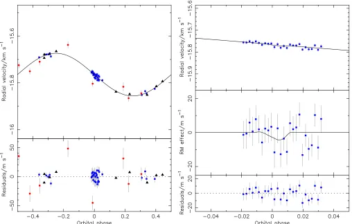
Our adopted model thus uses the combination of a circular orbit and no long-term RV trend, with neither thevsinI nor stellar radius priors applied. This model provides values of λ = 8◦.6+6.4
−6.5,vsinI = 3.9±0.5 km s−1 (slightly slower than the value from spectroscopic analysis),b = 0.66±0.02, and i=85◦.1±0.2. The resulting RV curve is displayed in Figure1 alongside a close-up of the transit region, showing the RM anomaly. The amplitude of the anomaly is low owing to the moderate rotation speed of the host star, but the signal-to-noise ratio is high and the anomaly is well constrained. We found that the semiamplitudes returned for all three of the RV data sets (the CORALIE data from Maxted et al. 2010, our new HARPS out-of-transit data, and our HARPS in-transit data) were in good agreement and consistent with the results from the discovery paper. Our barycentric velocities, on the other hand, while consistent with each other, are slightly less than the value found by Maxted et al. (2010), even for their CORALIE spectroscopy.
3.2. Doppler Tomography
The set of priors identified as composing the best-fitting model for our RM analysis were applied to our Doppler tomography method, allowing us to assess a single model only. Figure2 displays the residual maps from our analysis, which returned values ofvsinI =3.9+0.4
−0.5km s−1andλ=10◦.5+6
.4
Figure 1.Results from our adopted model for WASP-32:e=0, no long-term radial velocity trend; no prior on the spectroscopicvsinI, and no stellar radius prior. The best-fitting model is plotted as a solid black line. Top left: complete radial velocity reflex motion curve. Data from CORALIE are denoted by triangles. Data from HARPS are denoted by squares. Error bars are marked in gray; some are smaller than the size of the data points that they accompany. Bottom left: residuals from the RV fit, exhibiting no correlation with phase. Top right: close-up of the transit region from the radial velocity curve showing the RM effect, along with the residuals. Middle right: close-up of the transit region, with the orbital contribution removed. Bottom right: residuals for the radial velocity data within the RM window. (A color version of this figure is available in the online journal.)
Figure 2.Left: residual map of WASP-32 time-series CCFs with the model stellar spectrum subtracted. The signature of the planet moves from bottom left to top right, supporting the aligned, prograde orbit conclusion from our RM analysis. Right: the best-fitting model for the time-variable planet feature has been subtracted, leaving the overall residual map. The lack of any features in this figure indicates a lack of large-scale stellar activity. The horizontal dotted line marks the mid-transit phase. The vertical dotted line denotes the stellar radial velocity, while the vertical dashed lines indicate±vsinIfrom this, effectively marking the position of the stellar limbs. The crosses mark the four contact points for the planetary transit.
a lack of significant stellar activity in the host star, as any such activity would produce signatures similar to that of the planet (e.g., non-radial pulsation in WASP-33; Collier Cameron et al. 2010b).
4. WASP-38
[image:5.612.57.561.457.638.2]Table 3
Out-of-transit RV Data for WASP-38 Obtained Using HARPS
BJDUTC(–2,450,000) RV σRV
(km s−1) (km s−1)
5656.783091 −9.51508 0.00337
5657.783221 −9.52550 0.00299
5660.811940 −9.98361 0.00319
5662.834946 −9.64728 0.00423
5680.716630 −9.95563 0.00389
5681.710237 −9.97538 0.00295
5683.728896 −9.59883 0.00285
5714.660893 −9.89326 0.00588
5716.602469 −9.90687 0.00307
5749.637217 −9.96974 0.00642
5753.648280 −9.50884 0.00481
5802.476558 −9.58648 0.00600
5806.489798 −9.80177 0.00370
5809.496470 −9.61798 0.00300
Teff =6180+40−60 K. Further information regarding its discovery can be found in Barros et al. (2011). Photometry from the WASP-N array, the RISE instrument mounted on the 2 m Liverpool Telescope (Steele et al. 2008; Gibson et al. 2008), and an 18 cm Takahashi astrograph at La Palma was combined with spectroscopic measurements taken using the CORALIE and SOPHIE instruments to confirm the presence of the planet.
The RM effect of WASP-38 b has been analyzed previously by Simpson et al. (2011), who obtained spectroscopic observations of a transit event using the FIES spectrograph mounted on the Nordic Optical Telescope at La Palma. Despite the low precision of their measurements, they were able to place useful constraints on the misalignment angle using the shape of the RV anomaly during transit, ruling out high angles and confining the system to prograde orbits. They reported a final value for the misalignment angle ofλ=15◦+33
−43 but were not able to provide firm conclusions as to the alignment, or otherwise, of the system. We obtained new spectroscopic observations using HARPS of the transit event on the night of 2011 June 15, as well as addi-tional observations made throughout 2011 to provide coverage of the entire RV curve (see Tables3and4). We again obtained photometric observations of a transit using TRAPPIST, on 2011 April 13, but unfortunately we were not able to obtain simulta-neous photometry of our spectroscopically observed event. As with WASP-32, we analyzed our new HARPS spectra to ob-tain a value forvsinI of 8.3±0.4 km s−1. A macroturbulence ofvmac =3.7±0.3 km s−1 was assumed, again using the cal-ibration of Bruntt et al. OurvsinI is in excellent agreement with the values ofvsinI =8.6±0.4 km s−1quoted by Barros et al. (2011) andvsinI =8.58±0.39 km s−1found by Simp-son et al. (2011). Our adoptedvmac is significantly lower than the 4.9±0.4 km s−1 that Barros et al. (2011) used to fit their spectroscopy. Barros et al. used the calibration of Gray (2008), whereas we used that of Bruntt et al. (2010). Reanalyzing our new spectra using the Gray calibration returns a slightly lower value ofvsinI =7.9±0.4 km s−1, in agreement with the Bar-ros et al. results. In spite of this, we feel that the Bruntt et al. calibration gives a better fit to our data, and it is therefore the result that we use for our spectroscopic prior.
4.1. Rossiter–McLaughlin Analysis
Our initial stellar “jitter” estimate of 1 m s−1 led to poorly constrained results, with the lowestχ2
[image:6.612.338.548.81.731.2]red value returned by any of the models being 1.7. We therefore recalculated the stellar
Table 4
In-transit RV Data for WASP-38 Obtained Using HARPS
BJDUTC(–2,450,000) RV σRV
(km s−1) (km s−1)
5727.508875 −9.72505 0.00658
5727.519373 −9.72057 0.00586
5727.523134 −9.71142 0.00564
5727.527081 −9.70382 0.00585
5727.530912 −9.69675 0.00523
5727.534824 −9.69758 0.00528
5727.538562 −9.69301 0.00529
5727.542879 −9.69153 0.00527
5727.546791 −9.69410 0.00599
5727.550656 −9.68355 0.00613
5727.554603 −9.68966 0.00672
5727.558272 −9.67696 0.00592
5727.562045 −9.69909 0.00646
5727.566397 −9.69542 0.00694
5727.570343 −9.68220 0.00618
5727.574140 −9.70082 0.00615
5727.578017 −9.69531 0.00609
5727.581882 −9.70552 0.00618
5727.585586 −9.70640 0.00618
5727.592484 −9.71415 0.00667
5727.596430 −9.72199 0.00718
5727.600203 −9.71776 0.00651
5727.604046 −9.73514 0.00681
5727.607923 −9.73209 0.00676
5727.611800 −9.73769 0.00745
5727.619335 −9.74676 0.00739
5727.623177 −9.75379 0.00724
5727.627020 −9.76161 0.00671
5727.630746 −9.76295 0.00678
5727.634589 −9.76762 0.00661
5727.638466 −9.76457 0.00690
5727.642667 −9.78228 0.00754
5727.646510 −9.77732 0.00655
5727.650422 −9.78573 0.00707
5727.654183 −9.78749 0.00695
5727.658164 −9.78420 0.00719
5727.661868 −9.79843 0.00745
5727.666231 −9.80281 0.00769
5727.670143 −9.79479 0.00621
5727.673905 −9.79231 0.00634
5727.677747 −9.79598 0.00576
5727.681543 −9.79677 0.00532
5727.685386 −9.80741 0.00569
5727.689656 −9.80222 0.00564
5727.693430 −9.79689 0.00612
5727.697226 −9.79349 0.00704
5727.701242 −9.78573 0.00693
5727.705049 −9.78707 0.00585
5727.708915 −9.78243 0.00568
5727.713197 −9.76337 0.00552
5727.716936 −9.77080 0.00593
5727.720871 −9.77108 0.00529
5727.724713 −9.76885 0.00528
5727.728544 −9.76841 0.00528
5727.732306 −9.76986 0.00514
5727.736484 −9.76921 0.00541
5727.740141 −9.76496 0.00641
5727.744192 −9.76324 0.00720
5727.747999 −9.77120 0.00705
5727.751981 −9.76748 0.00679
5727.755823 −9.76974 0.00648
5727.760256 −9.78057 0.00585
Figure 3.Radial velocity curve produced by our optimal model for the WASP-38 system. The model uses an eccentric orbit and a prior on the stellar radius, but no long-term radial velocity trend is found and the prior on the spectroscopicvsinIis not applied. Data from CORALIE are denoted by triangles. Data from SOPHIE are denoted by circles. Data from FIES are denoted by diamonds. Data from HARPS are denoted by squares. Error bars are marked in gray; some are smaller than the size of the data points that they accompany. Format as for Figure1.
(A color version of this figure is available in the online journal.)
“jitter” following Wright (2005), obtaining three distinct values. We found that in order to forceχ2
red ≈1 we had to apply the conservative, 20th percentile estimate of 2.1 m s−1 to our new HARPS data and the 80th percentile estimate of 6.6 m s−1 to the pre-existing FIES, CORALIE, and SOPHIE data.11
We found that applying the spectroscopic prior on vsinI made little difference to the quality of fit that we obtained, or to the values ofvsinI and λ that we obtained when compared to the equivalent case without the application of the prior. Similarly, applying a long-term RV trend had no effect on the results, and the magnitude of any possible trend was found to be insignificant at| ˙γ|<22 m s−1yr−1. The stellar radius prior, however, despite producing only a small change in the values ofχred2 , had a significant impact on the results that we obtained. Cases in which the prior was not applied saw average increases in the stellar mass and radius of 6% and 27%, respectively, over their equivalent cases in which the prior was applied, as well as an average decrease in the stellar density of 49%. Note that these changes do not necessarily match perfectly, as under our model the stellar density is calculated directly from the transit light curves and independently from the stellar mass and radius. Relaxing the prior also produced significant increases invsinI and substantially raised the impact parameter from
¯
b = 0.15+0−0..3330 to b¯ = 0.62+0
.11
−0.13. Furthermore, we found that removing the prior increased the value of the stellar radius penalty,S, fromS¯=14.0 toS¯=105.3.
11 For an explanation of these estimates, see Wright (2005).
Allowing the eccentricity to float led to a clear and significant difference in both χred2 and the total χ2 for the combined photometric and spectroscopic model. The values returned by our algorithm lie at 7σ from e = 0 and were found to be significant by theF-test of Lucy & Sweeney (1971). This confirms the eccentricity detection of Barros et al. (2011), and the values that we find are consistent with the value of e=0.0314+0.0046
−0.0041reported by those authors.
Our adopted model for this system therefore uses an eccentric orbit, does not include a long-term RV trend, does not apply a prior onvsinI, and does utilize a prior on the stellar mass. This model returns values ofλ=9.◦2+18.1
−15.5,vsinI =7.7+0
.5
−0.4km s−1 (slower than the spectroscopic result), b = 0.09+0−0..1306, and i=89◦.6+0.3
−0.6, all of which indicate a well-aligned system. The RV curves are displayed in Figure3. The difference in quality between the FIES data presented by Simpson et al. (2011) and our new HARPS measurements is immediately apparent, particularly during the first half of the transit. The shape of the anomaly is well defined, and it has the large amplitude that is expected given the host star’s rapid rotation. It also appears to be highly symmetric, lending credence to the conclusion that the system is likely well aligned.
Figure 4.Left: residual map of WASP-38 time-series CCFs with the model stellar spectrum subtracted. The bright signature of the planet is clearly visible, and its trajectory from bottom left to top right clearly indicates a prograde orbit. Right: the best-fitting model for the time-variable planet feature has been subtracted, leaving the overall residual map. The lack of any remaining signatures suggests that the star is chromospherically quiet. Details as for Figure2.
Table 5
Comparison of Results for WASP-38
Source vsinI λ b
(km s−1) (deg) (R
∗) Simpson et al. (2011) 8.58±0.39 15+33−43 0.27+0.10−0.14 This work: RM effect 7.7+0.5
−0.4 9.2+18.1−15.5 0.09+0.13−0.06 This work: tomography 7.5+0.1−0.2 7.5+4.7−6.1 0.12+0.08−0.07
(2011) have a much smaller semiamplitude than any of the other data sets: 0.152±0.030 km s−1 compared to values be-tween 0.246±0.001 and 0.255±0.007 km s−1. Interestingly, Simpson et al. found a semiamplitude of 0.2538±0.0035 km s−1 in their analysis, but we suspect that this was overwhelmingly derived from the SOPHIE and CORALIE data, which cover the entire orbital phase. The barycentric velocities agree well with the results of that previous study, however.
4.2. Doppler Tomography
We again used the set of priors adopted for our RM modeling as the basis for our Doppler tomography analysis, and Table5 displays the results from this analysis, together with the results from Simpson et al. (2011) and our own RM analysis. It is immediately apparent that we have been able to dramatically reduce the uncertainties on the projected spin–orbit alignment angle; we will return to the question of why this is in Section7. The signature of the planet is clearly defined in Figure4, and in the final residual image there is no sign of any anomalies in the stellar line profiles, indicating that the host star is chromospherically quiet.
5. HAT-P-27/WASP-40
HAT-P-27 (B´eky et al.2011) is a fairly typical hot Jupiter system, with a 0.6MJupplanet in a 3.04 day orbit around a late-G/early-K-type star with Teff = 5190+160
−170 K and super-solar metallicity. The system was characterized using photometry from HATnet and KeplerCam on the 1.2 m FLWO telescope and spectroscopy from HIRES. It was also independently
discovered by the WASP survey using the combined WASP-N and WASP-S arrays, together with spectroscopy from SOPHIE, and designated WASP-40 (Anderson et al.2011).
We obtained new spectroscopic measurements using HARPS of the transit on the night of 2011 May 12 and carried out additional observations at a range of orbital phases throughout 2011 May (see Table6). New photometric observations were also made using TRAPPIST on 2011 May 17, covering a full transit. We combined these new data with those from both B´eky et al. (2011) and Anderson et al. (2011) for our attempt to characterize the RM effect.
As for WASP-38, we found that our original estimate of 1 m s−1 for the stellar “jitter” produced poorly constrained (χ2
red≈1.7) models. We calculated possible values of 5.9 m s−1 (20th percentile), 7.5 m s−1 (median), and 9.8 m s−1 (80th percentile) using the method of Wright (2005) and apply the latter to the existing SOPHIE data. We also note that B´eky et al. (2011) applied a “jitter” of 6.3 m s−1 to their HIRES data. To confirm that this was reasonable, we analyzed the photometric data in conjunction with only the HIRES spectroscopic data, finding that our initial estimate of 1 m s−1 produced χ2
red = 10.0±1.5, the 20th percentile value producedχred2 =1.1±0.5, the median value produced χ2
red = 0.7±0.4, and the 80th percentile value producedχred2 =0.4±0.3, while applying their estimate producedχ2
red =1.0±0.5. We therefore follow B´eky et al. and apply a “jitter” of 6.3 m s−1to the HIRES data.
[image:8.612.40.297.315.384.2]Figure 5.Results from the fit to the radial velocity data for our adopted solution for WASP-40. A circular orbit was used, with no prior on the spectroscopicvsinI, no long-term radial velocity trend, and no prior on the stellar radius. Data from HIRES are denoted by triangles. Data from SOPHIE are denoted by circles. Data from HARPS are denoted by squares. Error bars are marked in gray; some are smaller than the size of the data points that they accompany. Format as for Figure1. (A color version of this figure is available in the online journal.)
As with our RM analysis of WASP-32, we found that there was little to separate the different models for the WASP-40 system, as no significant differences were apparent in the values ofχ2
redthat we obtained. The eccentricities returned for models with non-circular orbits were found to be insignificant by the statistical test of Lucy & Sweeney (1971), and the values were all found to be consistent withe=0 to within 1.5σ. We also note that the addition of HARPS spectrographic measurements has reduced the value of any possible eccentricity in the system by a factor of 10 compared to the results in Anderson et al. (2011). The addition of a long-term RV trend to the model was found to provide no improvement in the quality of the fit obtained, and the low magnitude of any possible trend (| ˙γ|<43 m s−1yr−1) leads us to conclude that no such trend is present in the system. Imposing a prior on the stellar radius produced only small changes in the mass (|δM∗| 2%), radius (δR∗ 3%), and density (δρ∗7%) of the host star. The impact parameter was similarly unaffected, with only the error bars increasing with the relaxation of the prior.
Adding a prior onvsinI using the spectroscopic measure-ment produced no change in the value ofχred2 , but it significantly lowered the value ofvsinI returned by the MCMC algorithm and greatly reduced the uncertainties on the values of λ that were being produced. Examination of the HARPS spectroscopy indicated that the amplitude of any RM effect was likely to be low, with the error bars on the data such that they obscured any possible anomaly in the RV curve. This indicated that the value
ofvsinIwas likely to be low and that the error bars onλwould likely be high. This information, combined with the lack of any difference in the quality of fit, led us to select a solution in which the prior onvsinI was not applied.
Table 6
RV Data for WASP-40 Obtained Using HARPS
BJDUTC(–2,450,000) RV σRV
(km s−1) (km s−1)
5686.691040 −15.68740 0.00531
5691.594153 −15.83574 0.00593
5691.621178 −15.84591 0.00639
5691.784798 −15.82559 0.00548
5692.677700 −15.67883 0.00455
5692.747097 −15.67360 0.00411
5693.571851 −15.75439 0.00814
5693.577950 −15.75479 0.00878
5693.584107 −15.74939 0.00838
5693.590207 −15.75567 0.00843
5693.596480 −15.74962 0.00807
5693.602579 −15.75667 0.00803
5693.608737 −15.76548 0.00767
5693.614952 −15.75844 0.00817
5693.621167 −15.76064 0.00735
5693.627093 −15.75956 0.00822
5693.633296 −15.77570 0.00901
5693.639569 −15.76272 0.00858
5693.645669 −15.77900 0.00757
5693.651884 −15.77096 0.00700
5693.657925 −15.77981 0.00764
5693.664152 −15.76408 0.00737
5693.670263 −15.76868 0.00751
5693.676467 −15.76874 0.00774
5693.682682 −15.76226 0.00709
5693.688781 −15.78715 0.00662
5693.694927 −15.77673 0.00671
5693.701142 −15.78574 0.00677
5693.707184 −15.78466 0.00663
5693.713387 −15.76800 0.00666
5693.719603 −15.78821 0.00713
5693.725633 −15.77244 0.00792
5693.787541 −15.78723 0.00474
5694.567017 −15.85210 0.00448
5695.576799 −15.69093 0.00362
5695.757478 −15.67832 0.00406
angles are included in the possible range of solutions that we find.
In light of this, we analyzed the system using our preferred choice of priors and initial conditions, but with no RM effect fitting. We found that this produced results that showed no difference in terms of quality of fit from our adopted solution, with a value of χ2
red,noRM = 1.3±0.2 that is in complete agreement with χred2 = 1.3±0.2 from the solution adopted above. We therefore consider our weak constraints on the alignment angle to be equivalent to a non-detection of the RM effect.
5.1. Doppler Tomography
We attempted to model the system using Doppler tomog-raphy, but the combination of the low signal-to-noise ratio and slow rotation proved too difficult to analyze using this method. This nicely highlights a major limitation of the tech-nique, namely, systems with poor-quality spectroscopic data. RM analysis is able to overcome the poor data quality to pro-vide a result, although it may be inconclusive. However, the tomography method is simply unable to process the data if the effect of the planetary transit on the stellar line profile is insignificant.
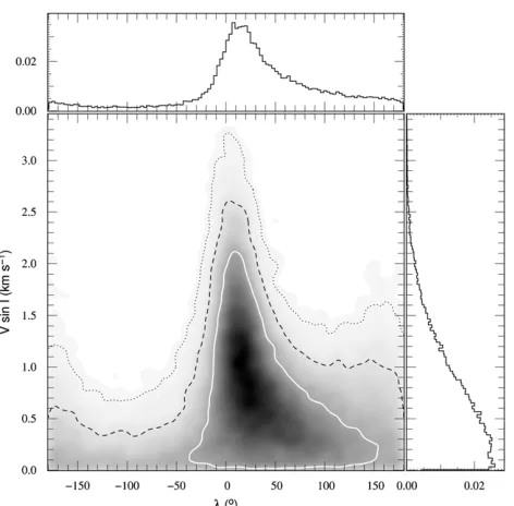
Figure 6.Posterior probability distribution forvsinIandλ, derived from the Markov Chain, for the fit to the data for WASP-40 described in Figure5. The white contour marks the 62.87% confidence regions, the black, dashed contour marks the 95.45% confidence regions, and the black, dotted contour marks the 99.73% confidence regions. Marginalized, one-dimensional distributions are displayed in the side panels.λ=0 lies well within the main body of the distribution.
6. OUR RESULTS IN CONTEXT
We now consider our new results, which are summarized in Table7, in the context of the complete set of spin–orbit align-ment measurealign-ments. To date, 52 systems have such measure-ments published; our results push that number up to 54.
6.1. Effect on Existing Trends with Mass and Temperature
In Brown et al. (2012), we updated the |λ| −Teff plot of Winn et al. (2010a) with all of the systems published since their original analysis and the results presented in our own work. Albrecht et al. (2012) carried out a similar exercise with their new measurements. We consider the new results presented herein in the context of the set of systems listed in the Holt–Rossiter–McLaughlin database compiled by Ren´e Heller,12as well as the new systems and results from Albrecht et al. (2012).
Our new results add little further information to the detected trend with temperature discovered by Winn et al. (2010a). The three systems that we study herein all fit into the “cool” category, although WASP-32 atTeff = 6100±100 lies close to the critical temperature dividing the two sub-populations, and WASP-38 atTeff =6110±150 encompasses the value of Tcrit = 6250 K within its 1σ Teff range. Similarly, our new results have no effect on the known trend with planetary mass as the systems all haveMp 3 MJup. They therefore cannot provide counterexamples, as planets in this category are already thought to exhibit randomly distributed values ofλ.
6.2. Stellar Ages
The host stars of WASP-32 and WASP-40 are insufficiently massive to fulfill the selection criterion imposed by Triaud (2011) for his study of the trend ofλwith stellar age. WASP-38
[image:10.612.73.268.75.464.2]Table 7
Summary of Results for WASP-32, WASP-38, and WASP-40
Parameter Units WASP-32a WASP-38a WASP-40b
Fitted parameters
D 0.0108±0.0001 0.0069±0.0001 0.0143±0.0005
K m s−1 0.478±0.011 0.252±0.004 0.0912±0.002
b R∗ 0.66±0.02 0.12+0.08
−0.07 0.87±0.01
W days 0.0990±0.0007 0.1969±0.0010 0.070+0.001
−0.002
P days 2.718661±0.000002 6.87188±0.00001 3.039577+0.000005
−0.000006
T0 BJ DUTC−2450000 5681.1945±0.0002 5322.1774±0.0006 5407.9088±0.0002 Derived parameters
Rp/R∗ 0.104±0.005 0.083±0.002 0.120+0.009
−0.007
R∗/a 0.129±0.003 0.0829+0.0008−0.0007 0.102+0.003−0.004
R∗ R 1.09±0.03 1.35±0.02 0.87±0.04
M∗ M 1.07±0.05 1.23±0.04 0.92±0.06
ρ∗ ρ 0.84±0.05 0.50±0.01 1.38+0.16−0.13
[Fe/H] -0.13±0.10 -0.02±0.07 0.14±0.11
vsinI km s−1 3.9+0.4−0.5 7.5+0.1−0.2 0.6+0.7−0.4
Rp RJup,eq 1.10±0.04 1.09±0.02 1.02+0.07−0.06
Mp MJup 3.46+0.14−0.12 2.71±0.07 0.62±0.03
a AU 0.0390±0.0006 0.0758±0.0008 0.0400±0.0008
i deg 85.1±0.2 89.5+0.3
−0.4 85.0±0.2
e 0(adopted) 0.028±0.003 0(adopted)
ω deg 0 −22.2+9.2
−8.1 0
λ deg 10.5+6.4
−5.9 7.5
+4.7
−6.1 24.2+76.0−44.5
| ˙γ| m s yr−1 0(adopted) 0(adopted) 0(adopted)
Notes.
[image:11.612.44.296.429.510.2]aResults from Doppler tomography. bResults from Rossiter–McLaughlin analysis.
Table 8
Age Estimates for the Three Systems
System Stellar Model Fitting Age Gyrochronology
Padova Y2 Teramo VRSS Age
(Gyr) (Gyr) (Gyr) (Gyr) (Gyr)
WASP-32 2.36+1.72−0.85 2.22+0.62−0.73 4.50+1.88−1.69 1.41+1.36−1.10 2.42+0.53−0.56 WASP-38 3.41+0.48
−0.43 3.29+0.42−0.53 3.59+0.77−0.70 3.20+0.73−0.59 3.41+0.26−0.24 WASP-40 >1.20 6.36+5.86−3.11 >4.96 >5.73 3.60+1.78−1.84
lies close to the cutoff mass; in some of our simulations it falls below the limit, but in our adopted solution it fulfills Triaud’s criterion for inclusion. We computed the ages for our three systems using a simple isochrone interpolation routine and several different sets of stellar models, in an attempt to better characterize the inherent uncertainties. Specifically, we made use of the Padova models (Marigo et al.2008; Girardi et al.2010), Yonsei-Yale (Y2) models (Demarque et al.2004), Teramo models (Pietrinferni et al.2004), and Victoria-Regina Stellar Structure (VRSS) models (VandenBerg et al. 2006). We carried out our isochrone fits in ρ∗−1/3–Teff space, taking the effective temperature from spectroscopic analysis of the HARPS spectra and the stellar density value as found by our preferred model under the tomographic method for WASP-32 and WASP-38 and the RM model for WASP-40. The ages that we obtained for the three systems using these models are set out in Table8. We also assessed the ages of the systems using a combination of theRHK activity metric and gyrochronology. We measured the chromospheric CaiiH & K emission from the new
HARPS spectra that we obtained for the three systems discussed herein, using this to calculate log(RHK ). We then computed the stellar rotation period using the method of Watson et al. (2010), which in turn allowed us to estimate the age of the system using the method of Barnes (2007), coupled with the improved coefficients of Meibom et al. (2009) and James et al. (2010).
to the arbitrary cutoff of Triaud (2011), so we might expect that the age would be better constrained. Nevertheless, our four age estimates for WASP-38 all agree with the postulated trend for alignment angle to decrease with time.
Finally, WASP-40 is poorly constrained, and we are unable to place upper limits on the age using the available isochrones for three out of the four model sets that we tried. It is hard to conclude anything from this, but the different models do agree that the system is older than either WASP-32 or WASP-38. On the other hand, we note that the gyrochronological estimate of the stellar age is significantly lower than the age limit that we found from our isochronal fits to the Teramo and VRSS models, although it is consistent with the results from the Y2and Padova models. Anderson et al. (2011) found ages for the system of 6±5 Gyr using the stellar models of Marigo et al. (2008) and Bertelli et al. (2008), which is consistent with our values. They too found a lower age (1.2+1−0..38 Gyr) using gyrochronology, in their case based on an estimate of the rotation period derived fromvsinI, but this does not match our estimate. From this information we tentatively predict, following the trend noticed by Triaud (2011), that the system will prove to be aligned if the uncertainty onλis able to be reduced.
6.3. Are the Systems Aligned?
In Brown et al. (2012), we introduced a new test for misalign-ment that is based on the Bayesian information criterion (BIC). The BIC is calculated for the set of RV measurements that fall within the transit window, for both the best-fitting model and one that assumes an aligned orbit withλ = 0◦. The ratio,B, of the aligned orbit BIC to the free-λ BIC is then calculated. Systems withB 0.99 are classed as aligned, systems with B 1.01 are classed as misaligned, and systems that fall be-tween these limits are classed as indeterminate. Albrecht et al. (2012) note that the BIC test is affected by the relative numbers of RV measurements in transit compared to out of transit, and that it assumes that no correlated noise is present. We acknowl-edge that these are indeed shortcomings of our test and that they might affect the boundaries between the three categories discussed in Brown et al. (2012), but we comment that the test is still quantitative, as opposed to the qualitative nature of the previous tests in Triaud et al. (2010) and Winn et al. (2010a).
We applied this test to our new results, calculating val-ues of 0.92 for WASP-32, indicating alignment; 0.95 for WASP-38, indicating alignment; and 0.97 for WASP-40, in-dicating alignment. However, in Brown et al. (2012), we also postulated a fourth category, that of “no detection,” defining this asvsinI consistent with 0 to within 1σ. With further reflection, we consider this definition to be inadequate. Our analysis rou-tines are set up in such a way that such a scenario is highly unlikely to exist; indeed, a lower error bar onvsinI of greater magnitude than the value itself is nonsensical, as negative ro-tation is a physical impossibility when considering only the magnitude of the rotation. We therefore revise this category of “no detection” to include systems withvsinI consistent with 0 to within 2σ. This new definition encompasses WASP-40, as we feel is appropriate given the poor signal-to-noise ratio of the data that we obtained and the indistinct RM effect that we find. The amended category includes no additional systems from our previous sample (see Brown et al.2012for details), although WASP-1 and WASP-16 are close, but would include the re-sults for TrES-2 (Winn et al.2008) and HAT-P-11 (Winn et al. 2010b).
6.4. Tidal Timescales
Albrecht et al. (2012) present two different approaches for estimating the tidal evolution timescales for hot Jupiter systems and calculate said timescale for a large sample of planets for which the RM effect has been measured. They take two approaches. In the first, they consider a bimodal sample of planets: those with convective envelopes and those with radiative envelopes. In the second approach they consider the mass of the convective envelope, which they link to stellar effective temperature. Unfortunately, this second approach relies on an unspecified proportionality constant, and the relation between Teff andMCZ that they derived is also unknown. We therefore consider their first approach, which is encapsulated in the equations
1 τCE
= 1
10×109yrq 2
a/R∗ 40
−6
(2)
and
1 τRA =
1
0.25×5×109yrq
2(1 +q)5/6
a/R∗ 6
−17/2 . (3)
The stellar effective temperatures of our three systems are, as mentioned previously, below the critical temperature divid-ing the “hot” and “cool” regions of parameter space. They therefore all fall under the convective envelope version of the tidal timescale equation. Using parameters from our best-fitting models (tomographic for WASP-32 and WASP-38 and RM for WSAP-40), we calculate the tidal timescales for our three systems using Equation (2). We find τCE = 5.46867636× 10¹⁰yr for WASP-32, τCE = 1.79351519 × 10¹²yr for WASP-38, and τCE = 5.41028372×10¹²yr for WASP-40. These values fit nicely into the scheme that Albrecht et al. (2012) developed, whereby systems in which the tidal timescale is short preferentially show low values ofλ, whereas those with longer timescales appear to present an almost random distribution ofλ. The timescales for our three systems are relatively short, partic-ularly where WASP-32 is concerned, and the small alignment angle that we obtained for that system is exactly as expected.
7. WHY USE DOPPLER TOMOGRAPHY?
As we discussed in Section1, Doppler tomography is one of a number of methods for characterizing spin–orbit alignment that are beginning to be used as alternatives to the traditional RV-based approach that we have used to analyze all three of the systems in this study. Although tomography has weaknesses and cannot be applied to every planetary system (as witnessed with WASP-40 previously), it has one great selling point over the RV method. Tomography is able to lift the strong degeneracy that exists betweenvsinI andλ, and which is strongest in systems with low impact parameter.
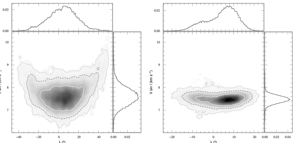
Figure 7.Posterior probability distributions forvsinIandλfor both of the analysis methods discussed in this work. These distributions are for the analysis of the WASP-38 system discussed in Section4. Key as for Figure6. Left: radial-velocity-measurement-based Rossiter–McLaughlin analysis. Right: Doppler tomography. The difference between the two methods is stark, with the tomographic analysis yielding a much reduced correlation between the parameters.
This is not the only parameter involved, however. The stellar rotation,vsinI, dictates the amplitude of the RM anomaly, but this is often ambiguous owing to the uncertainties present in the RV measurements. It is often not clear, particularly for systems with lowvsinI, whether the anomaly is truly asymmetric or whether it is an effect produced by the error bars (see, for example, WASP-25 in Brown et al. 2012). This means that the same anomaly can often be fit in two different ways. Either vsinI is low andλindicates misalignment, with the resulting asymmetry in the model used to fit the uncertainties, orλis low and a rapidvsinI is used, with the greater amplitude providing the required fit. Often what results is a compromise solution, with large error bars on both parameters and some degree of degeneracy between them. This arises owing to the use of the RM effect to characterize both parameters simultaneously. The problem is exacerbated for systems with low signal-to-noise ratio, for which the range of possible models that fit the data is greatly increased owing to the greater relative size of the uncertainties, and for systems with low impact parameter, for the reasons discussed above.
The Doppler tomography method does not suffer from this same problem and is therefore able to provide better constraints onλin these problematic cases. Directly modeling the separate components of the CCF provides several separate constraints on the parameters involved in the model, and the geometric calculation of the position of the planet’s shadow on the stellar disk helps to remove ambiguity regarding λ. These two factors lift the degeneracy experienced with the traditional method.
WASP-38, as an example of a system with low impact parameter, provides a reasonable example of the advantages that the tomographic analysis method holds over the standard RV method. Table5clearly shows that the error bars onλhave been decreased by the use of Doppler tomography, and Figure7shows the change in the relationship between the values ofvsinI and λfor the two analysis methods. The two posterior probability density plots show completely different distributions, with that
for the RV method showing a clear correlation between the two parameters, with obvious degeneracies in the fitted values. The tomographic distribution, on the other hand, shows very little in the way of correlation, and although there is still some spread in theλdistribution, the range ofvsinI values has quite clearly been heavily restricted.
8. CONCLUSIONS
We have presented measurements of the sky-projected spin–orbit alignment angle for the hot Jupiters WASP-32, WASP-38, and HAT-P-27/WASP-40, using both the RM ef-fect and Doppler tomography. We find that WASP-32 exhibits an alignment angle ofλ=10◦.5+6.4
−5.9(from Doppler tomography) and a rotation speed ofvsinI =3.9+0.4
−0.5km s−1, indicating an aligned system. The results from our two analysis methods are consistent and show good agreement, where applicable, with the original discovery paper. For HAT-P-27/WASP-40 we find a much lower rotation speed than suggested by the discovery paper and spectroscopic analysis,vsinI =0.6+0.7
−0.4km s−1, but our poor signal-to-noise data allow us to place only weak con-straints on the alignment angle. We findλ=24◦.2+76.0
−44.5, which we classify as a non-detection, and are unable to apply the to-mography method to the system. For WASP-38, we improve on the previous analysis of Simpson et al. (2011), reducing the uncertainty inλ by an order of magnitude, and obtaining λ=7◦.5+4.7
−6.1andvsinI =7.5+0
.1
−0.2km s−1through tomographic analysis. Our results again agree well between the two analysis methods.
Note added. We have used the UTC time standard and Barycentric Julian Dates in our analysis. Our results are based on the equatorial solar and Jovian radii and masses taken from Allen’s Astrophysical Quantities.
The WASP Consortium consists of representatives from the Universities of Keele, Leicester, The Open University, Queens University Belfast and St. Andrews, along with the Isaac Newton Group (La Palma) and the Instituto de As-trofisica de Canarias (Tenerife). The SuperWASP and WASP-S cameras are operated with funds made available from Con-sortium Universities and the STFC. TRAPPIST is funded by the Belgian Fund for Scientific Research (Fond National de la Recherche Scientifique, FNRS) under the grant FRFC 2.5.594.09.F, with the participation of the Swiss National Sci-ence Foundation (SNF). R.F.D. is supported by CNES. M.G. is an FNRS Research Associate and acknowledges support from the Belgian Science Policy Office in the form of a Re-turn Grant. I.B. acknowledges the support of the European Research Council/European Community under the FP7 through a Starting Grant, as well from Funda¸c˜ao para a Ciˆencia e a Tecnologia (FCT), Portugal, through SFRH/BPD/81084/2011 and the project PTDC/CTE-AST/098528/2008. This research has made use of NASA’s Astrophysics Data System Biblio-graphic Services, the ArXiv preprint service hosted by Cor-nell University, and Ren´e Heller’s Holt–Rossiter–McLaughlin Encyclopaedia (www.aip.de/People/RHeller).
REFERENCES
Albrecht, S., Winn, J. N., Johnson, J. A., et al. 2011,ApJ,738, 50 Albrecht, S., Winn, J. N., Johnson, J. A., et al. 2012,ApJ,757, 18 Anderson, D. R., Barros, S. C. C., Boisse, I., et al. 2011,PASP,123, 555 Barker, A. J., & Ogilvie, G. I. 2009,MNRAS,395, 2268
Barnes, J. W., Linscott, E., & Shporer, A. 2011,ApJ,197, 10 Barnes, S. A. 2007,ApJ,669, 1167
Barros, S. C. C., Faedi, F., Collier Cameron, A., et al. 2011,A&A,525, A54 Bate, M. R., Lodato, G., & Pringle, J. E. 2010,MNRAS,401, 1505 B´eky, B., Bakos, G. ´A., Hartman, J., et al. 2011,ApJ,734, 109 Bertelli, G., Girardi, L., Marigo, P., & Nasi, E. 2008,A&A,484, 815 Brown, D. J. A., Collier Cameron, A., Anderson, D. R. A., et al. 2012,MNRAS,
423, 1503
Bruntt, H., Bedding, T. R., Quirion, P.-O., et al. 2010,MNRAS,405, 1907 Collier Cameron, A., Bruce, V. A., Miller, G. R. M., Triaud, A. H. M. J., &
Queloz, D. 2010a,MNRAS,403, 151
Collier Cameron, A., Guenther, E., Smalley, B., et al. 2010b,MNRAS,407, 507 Collier Cameron, A., Wilson, D. M., West, R. G., et al. 2007, MNRAS,
380, 1230
Demarque, P., Woo, J.-H., Kim, Y.-C., & Yi, S. K. 2004,ApJS,155, 667 Enoch, B., Collier Cameron, A., Parley, N. R., & Hebb, L. 2010, A&A,
516, A33
Fabrycky, D., & Tremaine, S. 2007,ApJ,669, 1298
Gandolfi, D., Collier Cameron, A., Anderson, D. R., et al. 2012,A&A,543, L5 Gibson, N. P. 2008,A&A,492, 603
Girardi, L., Williams, B. F., Gilbert, K. M., et al. 2010,ApJ,724, 1030 Goldreich, P., & Tremaine, S. 1980,ApJ,241, 425
Gray, D. F. 2008, The Observation and Analysis of Stellar Photospheres (Cambridge: Cambridge Univ. Press)
H´ebrard, G., Ehrenreich, D., Bouchy, F., et al. 2011,A&A,527, L11 Hellier, C., Anderson, D. R., Collier Cameron, A., et al. 2009, Nature,
460, 1098
Hirano, T., Suto, Y., Winn, J. N., et al. 2011,ApJ,742, 69 Holt, J. R. 1893, A&A, 12, 646
James, D. J., Barnes, S. A., Meibom, S., et al. 2010,A&A,515, A100 Jehin, E., Gillon, M., Queloz, D., et al. 2011, Messenger,145, 2 Johnson, J. A., Winn, J. N., Albrecht, S., et al. 2009,PASP,121, 1104 Kozai, Y. 1962,AJ,67, 591
Lai, D., Foucart, F., & Lin, D. N. C. 2011,MNRAS,412, 2790
Lendl, M., Anderson, D. R., Collier-Cameron, A., et al. 2012, A&A, 544, A72
Lidov, M. L. 1962,Planet. Space Sci.,9, 719 Lucy, L. B., & Sweeney, M. A. 1971,AJ,76, 544
Marigo, P., Girardi, L., Bressan, A., et al. 2008,A&A,482, 883
Maxted, P. F. L., Anderson, D. R., Collier Cameron, A., et al. 2010,PASP, 122, 1465
McLaughlin, D. B. 1924,ApJ,60, 22
Meibom, S., Mathieu, R. D., & Stassun, K. G. 2009,ApJ,695, 679
Miller, G. R. M., Collier Cameron, A., Simpson, E. K., et al. 2010,A&A, 523, A52
Nagasawa, M., Ida, S., Bessho, T., et al. 2008,ApJ,678, 498 Naoz, S., Farr, W. M., Lithwick, Y., et al. 2011,Nature,473, 187 Naoz, S., Farr, W. M., & Rasio, F. A. 2012,ApJ,754, L36 Narita, N., Sato, B., Hirano, T., & Tamura, M. 2009, PASJ,61, L35 Ohta, Y., Taruya, A., & Suto, Y. 2005,ApJ,622, 1118
Pepe, F., Mayor, M., Galland, F., et al. 2002,A&A,388, 632
Pietrinferni, A., Cassisi, S., Salaris, M., & Castelli, F. 2004,ApJ,612, 168 Pollacco, D., Skillen, I., Collier Cameron, A., et al. 2006,PASP,118, 1407 Queloz, D., Eggenberger, A., Mayor, M., et al. 2000, A&A,359, L13 Rogers, T. M., Lin, D. N. C., & Lau, H. H. B. 2012,ApJ,758, L6 Rossiter, R. A. 1924,ApJ,60, 15
Sanchis-Ojeda, R., Winn, J. N., Holman, M. J., et al. 2011,ApJ,733, 127 Sasselov, D. D., & Lecar, M. 2000,ApJ,528, 995
Schlaufman, K. C. 2010,ApJ,719, 602
Schlesinger, F. 1910, Publ. Allegheny Obs. Univ. Pittsburgh,1, 123 Schlesinger, F. 1916, Publ. Allegheny Obs. Univ. Pittsburgh,3, 23
Simpson, E. K., Pollacco, D., Collier Cameron, A., et al. 2011,MNRAS, 414, 3023
Southworth, J. 2009,MNRAS,394, 272 Southworth, J. 2011,MNRAS,417, 2166
Steele, I. A., Bates, S. D., Gibson, N., et al. 2008,Proc. SPIE,7014, 70146J Triaud, A. H. M. J. 2011,A&A,534, L6
Triaud, A. H. M. J., Collier Cameron, A., Queloz, D., et al. 2010,A&A, 524, A25
Valenti, J. A., & Fischer, D. A. 2005,ApJS,159, 141
VandenBerg, D. A., Bergbusch, P. A., & Dowler, P. D. 2006,APJS,162, 375 Watson, C. A., Littlefair, S. P., Collier Cameron, A., Dhillon, V. S., & Simpson,
E. K. 2010,MNRAS,408, 1606
Watson, C. A., Littlefair, S. P., Diamond, C., et al. 2011,MNRAS,413, L71 Weidenschilling, S. J., & Marzari, F. 1996,Nature,384, 619
Winn, J. N., Fabrycky, D., Albrecht, S., & Johnson, J. A. 2010a, ApJ, 718, L145