Physical insight into the accuracy of finely-resolved iLES in turbulent boundary layers

Physical insight into the accuracy of finely-resolved iLES in turbulent

boundary layers

Konstantinos Ritos, Ioannis W. Kokkinakis, Dimitris Drikakis

PII:

S0045-7930(17)30256-6

DOI:

10.1016/j.compfluid.2017.07.018

Reference:

CAF 3551

To appear in:

Computers and Fluids

Received date:

14 March 2017

Revised date:

5 July 2017

Accepted date:

19 July 2017

Please cite this article as: Konstantinos Ritos, Ioannis W. Kokkinakis, Dimitris Drikakis, Physical insight

into the accuracy of finely-resolved iLES in turbulent boundary layers,

Computers and Fluids

(2017),

doi:

10.1016/j.compfluid.2017.07.018

ACCEPTED MANUSCRIPT

Highlights

• Physical insight into the accuracy of iLES methods for turbulent boundary layers.

• Order of accuracy in iLES affects turbulence anisotropy and symmetry.

• Highest anisotropy correlates with maximum Reynolds stress and mini-mum flatness.

ACCEPTED MANUSCRIPT

Physical insight into the accuracy of finely-resolved

iLES in turbulent boundary layers.

Konstantinos Ritos1,∗_{, Ioannis W. Kokkinakis}a_{, Dimitris Drikakis}a

a_{University of Strathclyde, Glasgow, G1 1XJ, UK}

Abstract

This paper investigates the numerical accuracy of implicit Large Eddy

Sim-ulations (iLES) in relation to compressible turbulent boundary layers (TBL).

iLES are conducted in conjunction with Monotonic Upstream-Centred Scheme

for Conservation Laws (MUSCL) and Weighted Essentially Non-Oscillatory

(WENO), ranging from 2nd to 9th-order. The accuracy effects are presented

from a physical perspective showing skewness, flatness and anisotropy

calcu-lations, among others. The order of the scheme directly affects the physical

representation of the TBL, especially the degree of asymmetry and anisotropy

in the sub-layers of the TBL. The study concludes that high-order iLES can

provide an accurate and detailed description of TBL directly comparable to

available DNS and experimental results.

Keywords: iLES, High-Order, TBL, Supersonic

1. Introduction

Design processes in engineering applications require satisfying various

con-straints in order to adhere to design quality standards. Through careful planning

and availability of instrumentation/apparatus that conform to the necessary

specifications, experimental results can considerably assist during the design

5

stage. However, most experiments are deemed cumbersome and require

consid-erable time to plan, execute and later analyse. This is particularly true when

∗_{Corresponding author}

ACCEPTED MANUSCRIPT

an iterative process or optimization approach is required early on in the

de-sign phase. Furthermore, availability of diagnostic instrumentation limits the

amount of useful information that can be extracted.

10

Computational methods offer the possibility of a high turnover of results

and ample amounts of available data, allowing for a plethora of variations to

the initial design of a product to be investigated. They are increasingly

becom-ing more popular and widely used from simple low speed flows to hypersonic

aerodynamics and heat transfer studies of complex geometries [1]. However,

15

they are still treated with some caution and due care as the solutions provided

can contain significant inaccuracies. For example in fluid flow simulations these

are caused mostly by the number of assumptions associated with turbulence

modelling as well as the excessive numerical dissipation of schemes particularly

when simulations are performed on coarse grids.

20

In an effort to combine the high fidelity of Direct Numerical Simulation

(DNS) with the computational efficiency of classical Large Eddy Simulation

(LES) led to the development of implicit LES (iLES). This concept emerged

from observations reported by Boris et al. [2] and has been applied successfully

to model several complex flows in engineering and other fields. The use of iLES

25

in free and wall-bounded flows has been justified by Fureby and Grinstein [3],

while a validation of the method through theoretical analysis has been presented

by Margolin et al. [4]. In incompressible flows, it is possible to develop an

op-timised stencil with regard to numerical dissipation [5], however, in the case

of compressible flows the numerical method should be monotonic with respect

30

to the thermodynamics quantities. More recently, Kokkinakis and Drikakis [6]

presented iLES results of a weakly compressible turbulent channel flow,

conclud-ing that iLES can achieve near DNS accuracy while utilisconclud-ing significantly less

computational resources. At the same time, and independently of [6], Poggie

et al. [7] applied compressible iLES to study TBL flows resulting in the same

35

conclusions.

In this paper, the accuracy of high-order, shock-capturing schemes along

tur-ACCEPTED MANUSCRIPT

bulent boundary layer (TBL) flows. The effects of numerical dissipation for

schemes with accuracy ranging from 2nd to 9th-order are investigated in

su-40

personic TBL. The accuracy of each iLES variant is scrutinised through the

calculation of higher-order statistics, i.e. skewness, flatness, and their direct

comparison with available DNS and experimental data. The results show that

higher order iLES schemes are particularly well suited for simulating TBL and

also highlight their capability to provide a physical insight in near-wall

super-45

sonic flows.

2. The Simulation Case

The in-house block-structured grid code CNS3D is used to solve the

Navier-Stokes equations using a finite volume Godunov-type method for the

convec-tive terms. The inter-cell numerical fluxes of the convecconvec-tive terms are

calcu-50

lated by solving the Riemann problem using the reconstructed values of the

primitive variables at the cell interfaces. The reconstruction stencil is a

one-dimensional swept unidirectional stencil. The Riemann problem is solved using

the so-called Harten, Lax, van Leer, and (the missing) Contact (HLLC)

approx-imate Riemann solver [8, 9]. Two different flux limiting approaches have been

55

implemented in conjunction with the HLLC solver, namely the: (i) Monotone

Upstream-centred Schemes for Conservation Laws (MUSCL) and (ii)

Weighted-Essentially-Non-Oscillatory (WENO). Titarev and Toro [10] investigated the

accuracy of WENO schemes with HLLC , but not within the iLES framework.

The flow physics are analysed with three variations of the iLES approach,

60

with their accuracy ranging from 2nd _{to 9}th _{order. In particular, these are}

the MUSCL piecewise linear 2nd_{-order limiter [11] (henceforth labeled M2), the}

MUSCL 5th_{-order limiter [12] (henceforth labeled M5), and the WENO 9}th

-order scheme [13] (henceforth labeled W9). The viscous terms are discretised

by a second-order central scheme. The solution is advanced in time by using

65

a five-stage (fourth-order accurate) optimal strong-stability-preserving

ACCEPTED MANUSCRIPT

L u∞ T∞ M P∞

0.061 m 588 m/s 170 K 2.25 23.8 kPa

ρ∞ Tw/T∞ µ∞ T u ReL

0.488 kg/m3 _{1.9 1.167×10}−5 _{Pa s 3% 1.5×10}6

Table 1: Simulation parameters. u∞, T∞, M, P∞, ρ∞, µ∞ are the freestream velocity, temperature, Mach number, pressure, density and viscosity, respectively. Tw is the wall

temperature,T u is the turbulence intensity at the inlet andReL is the Reynolds number

based on the freestream properties and the length of the plate (L).

given in [6] and [15] and references therein.

The simulation is set up similarly to that used in the study of Poggie et al. [7]

for ease of comparison with other numerical and experimental data produced

70

under similar flow conditions. A supersonic flow over a flat plate at Mach

number M = 2.25 that is fully turbulent in the region close to the outlet is

considered. Based on the freestream properties and the length of the plate (L),

the incoming flow has a Reynolds number of 1.5×106_{. Further flow parameters}

are given in Table 1.

75

Periodic boundary conditions are used in the spanwise (z) direction. In the

wall-normal (y) direction, a no-slip isothermal wall (with a temperature Tw

of 323 K) is used similar to [16]. High-order implementation of the boundary

conditions requires fictitious cells to be added inside the wall. The velocity

components on these cells are linearly extrapolated from the computational

80

cells inside the domain. The temperature is linearly extrapolated using the

specified wall temperature, while the density is calculated from the equation of

state considering zero pressure gradient normal to the wall. Supersonic outflow

conditions are imposed at the outlet, while far-field conditions are applied on the

upper boundary opposite of the wall. A synthetic turbulent inflow boundary

85

condition is used to produce a freestream flow with a superimposed random

turbulence.

ACCEPTED MANUSCRIPT

filter (DF) method documented in [17, 18, 19, 20, 21] and, specifically validated

in the framework of the present iLES code CNS3D in [20, 21]. According to

90

DF, instead of using a white-noise random perturbation at the inlet, energy

modes within the Kolmogorov inertial range scaling with k−5/3_{, where k is}

the wavenumber, are introduced into the turbulent boundary layer. No

large-scale energy modes scaling with k4 _{are introduced. A cutoff at the maximum}

frequency of 50 MHz is applied, since the finest mesh used in this study would

95

under-resolve higher values. The turbulence intensity at the inlet (T u) is set

as±3% of the intensity of the freestream velocity. This perturbation has been

found to be sufficient to trigger bypass transition and turbulence inside the

simulation domain (Fig. 1).

The number of mesh points and the mesh spacing are given in Table 2. The

100

iLES calculations are performed on relatively fine meshes but still coarser than

required for DNS [7, 22]. This is highlighted in Table 2, where information

about the meshes used in previous DNS studies is included for comparison and

validation. The present mesh spacing (∆y) is scaled using the conventional

inner variable method ∆y+_=u

τ∆y/νw, whereuτ = p

(τw/ρw) is the friction 105

velocity,νw the near wall kinematic viscosity,τw the near wall shear stress, and

ρw the near wall density.

nx ny nz ∆x+ ∆yw+ ∆y+e ∆z+

iLES 2591 277 139 9.06 0.497 6.26 8.53

DNS1[22] 1920 171 200 4.95-5.22 0.7 4.72-6.51 4.27-4.51

DNS2[22] 4160 221 440 5.58-5.86 0.7 9.42-12.35 4.75-4.99

DNS3[7] 22548 1277 1131 1.0 0.9 0.9 1.0

Table 2: Mesh parameters; nx, nyand nzare the number of mesh points. The ‘+’ sign denotes

dimensionless mesh spacing, as defined for ∆y+_{in the text. The subscripts ‘w’ and ‘e’ denote}

wall and boundary layer edge values, respectively.

In the next section, coarser meshes have been used to assess mesh

ACCEPTED MANUSCRIPT

Figure 1: Iso-surfaces ofQ-criterion,Q= 2(U∞/δ0)2, coloured by Mach number for all iLES

variants. Only a limited portion of the flow domain is shown on the left and zoom in the final

10% of the domain on the right.

been conducted by using the finest mesh resolution (see Table 2), which can

110

be considered as an under-resolved DNS. Following this approach we were able

to discern that even at finer mesh resolutions the results are dependent on the

order of the scheme. Numerical stability issues associated with the W9 scheme

at finer mesh resolutions require further investigation by performing resolved

DNS. This is beyond the scope of the present study.

ACCEPTED MANUSCRIPT

All of the calculations shown below are performed at the end of the plate in

the fully turbulent region, where the boundary layer has the properties presented

in Table 3. Various definitions of the Reynolds number are used in Table 3, i.e.,

Reθ=ρ∞U∞θ/µ∞,Reτ =ρwuτδ/µw, andReδ2=ρ∞U∞θ/µw, to simplify the

comparison of the present results with those of past and future publications. The

120

momentum and boundary layer thicknesses are denoted byθandδ, respectively.

The flow statistics at the calculation point are computed by averaging in time

over three flow cycles and spatially in the spanwise direction. The statistical

convergence of the simulations based on the Standard Error of the Mean (SEM),

is less than 2%. The total simulation time for each case is equal to six flow

125

cycles, with the first three omitted from the calculations for statistical purposes.

Statistical convergence in the calculations has been achieved and averaging over

a longer period would not adversely impact on the accuracy. Furthermore,

comparing the present results against theoretical models, DNS and experiments

tested the accuracy of iLES.

130

Reθ Reτ Reδ2 H M

W9 2170.0 414.0 1280.6 3.56 2.25

M5 1806.2 377.1 1065.9 3.51 2.25

M2 1593.8 344.6 940.5 3.72 2.25

DNS1[22] 1122.0 251.0 715 3.08 2.0

DNS2[22] 2377.0 497.0 1516.0 2.98 2.0

DNS3[7] - - 2000.0 - 2.25

Exp1[23] 4700.0 1050.0 2800 3.46 2.32

Exp2[24] 2400.0 501.0 1200.0 5.49 2.9

Exp3[25] 5100.0 1080.0 3100.0 2.00 2.28

Table 3: Boundary layer properties at the point of analysis. The same properties from previous DNS and experimental studies are also presented. The compressible form of the momentum

thickness (θ) has been used. H =δ∗_{/θis the shape factor, where (δ}∗_{) is the displacement}

ACCEPTED MANUSCRIPT

3. Physical Insight into Numerical Accuracy

The assessment of the various iLES approaches begins with basic flow

statis-tics for which a plethora of theoretical, numerical and experimental data are

available. A characteristic example is the van Driest velocity profile of the

TBL,

uV D=

Z u+

0

r _ρ

ρwdu

+ ₍₁₎

where the superscript ‘+’ denotes the usual wall scaling u+_=u/u

τ. The

nor-malised van Driest velocity profile by its value on the edge of the boundary layer

is presented in Fig. 2 along with previous DNS calculations and experimental

measurements. Previous publications [22, 26] have shown that for adiabatic

135

walls a satisfactory collapse of the data is expected in the overlap layer, and

also in the viscous sublayer. Small variations are expected for different Reynolds

number and all present iLES calculations should appear in-between the DNS

calculations of Pirozzoli et al.[22]. Only the high-order W9 satisfies this

expec-tation and it also perfectly collapses to previous experimental measurements

140

[24, 25].

The iLES results presented in Fig. 2 and in all of the following figures are

from simulations utilising the same mesh and simulation parameters, restricting

the source of any observable differences to the accuracy of the iLES variant. To

support this argument and to highlight the absence of mesh resolution effects

Fig. 3a shows the van Driest transformed velocity profiles for different mesh

resolutions. The results on mesh G3, which consists of ∼ 36 million points,

differ by less than 2% from those obtained by the finest mesh (G4) consisting of

∼100 million points. The average error of the present simulations in comparison to the DNS results of Pirozzoli et al.[22] is calculated using the results from Figs.

2 and 3a,

εAvg= 1

N

N X

i=1

ku¯DN S,i−u¯iLES,ik

¯

uDN S,i , (2)

where N is the number of points used in the calculation of the average error.

ACCEPTED MANUSCRIPT

0

0.2

0.4

0.6

0.8

1

0

0.2 0.4 0.6 0.8

1

1.2 1.4

1-u

/u

e

y

/

δ

DNS1

DNS2

Exp2

Exp3

iLES-W9

iLES-M5

iLES-M2

Figure 2: Comparison of van-Driest-transformed mean velocity with reference DNS and

ex-perimental data (see table 3).

average value in various points. Both the mesh size and the iLES order

signif-icantly affect the computational cost of the simulation. For each iLES variant

145

the computational cost is normalized by the computational time of W9 on the

coarsest mesh (G1). The W9 simulations on the coarser mesh G2 (∼10.5 million

mesh points) can achieve similar accuracy to the finest mesh (G4) simulations

of M5 and M2, thus reducing the computational cost by approximately

eight-fold. An extrapolated estimate of the computational cost that a DNS simulation

150

would require is made based on the results of Fig. 3b using the W9 and found

that the present iLES simulations are∼5 times less computationally expensive.

Other physical features of the TBL can be studied along with the effect

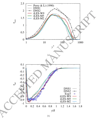
of the accuracy of the method on them. For example the attached-eddy

hy-pothesis [27, 28] predicts that logarithmic layers are formed for the variance of

attached variables accompanying an equilibrium layer. Perry & Li [29], based

ACCEPTED MANUSCRIPT

0 0.2 0.4 0.6 0.8 1

0 0.2 0.4 0.6 0.8 1 1.2 1.4

1-uVD /uVD

e

y/

δ

G4 - 2591x277x139 G3 - 1727x227x92 G2 - 1151x151x61 G1 - 864x114x47

(a)

0 5 10 15 20 25 30 35 40

0.5 5 50 500

ε

(%)

Normalised computational cost G1

G2

G3 _G4

G4

G4 DNS2 iLES-W9 iLES-M5 iLES-M2

(b)

Figure 3: (a) Effect of mesh refinement on accuracy, van-Driest-transformed mean velocity,

all results are from simulation utilising the W9 scheme. (b) Accuracy and computational

cost comparison between different iLES variants and meshes used. The DNS simulation of Pirozzoli et al.[22] (see tables 2 and 3) has been used as the reference, error bars show the

ACCEPTED MANUSCRIPT

fluctuations should scale as

u02

i

u2

τ

=Bi−Ailog(y/δ)−V(y+), (3)

where u0

i can be any of the fluctuating velocity components (u0, v0, or w0),

Bu = 2.39, Au = 1.03, Bw = 1.20. Aw = 0.475, while V(y+) accounts for

viscous corrections. The Reynolds normal and shear stressesτij=ρu0iuj0/(ρwu2τ) 155

are a common way to present the fluctuating velocity statistics (Figs. 4 and 5).

The two MUSCL variants of iLES significantly over-predict theτuu(Fig. 4a)

especially the peak region in the buffer zone of the TBL. However, the highest

order iLES (W9) has a very good agreement with all previous DNS results up

to abouty+_{≈20 where the Reynolds similarity holds [30]. Further away from}

160

the wall it is typical to observe a strong dependence on Reynolds number for

results presented in inner scaling. This can explain the observed differences in

the logarithmic region between the various results because the local Reynolds

number is not equal. It is also notable that W9 is the only iLES variant that

produces the correct scaling of τuu in the logarithmic region according to the 165

quantitative prediction of Perry & Li [29] (Eq. 3 withV = 0).

The effect of the iLES order is also noticeable in the calculation ofτvvwhere

the low order schemes significantly under-predict it in the whole range of the

boundary layer (Fig. 4b). This observation can be associated with unresolved

turbulent scales that produce the small near-wall fluctuations. The W9 results

170

along with the previously published DNS show a trend to Reynolds similarity

fory+_{<40. For higher values ofy}+_{, the Reynolds number dependence becomes}

obvious.

In the presentation ofτww(Fig. 5a) the accuracy of the iLES affects only the

logarithmic region, where the two MUSCL schemes under-predict the value of

175

the normal Reynolds stress. For distances up toy+_{≈30 all simulations confirm}

the Reynolds independence. The present results of normal Reynolds stresses

support the argument of Pirozzoli et al. [22] that turbulence dynamics over the

whole TBL have an incompressible behaviour because the present observations

agree very well with those made in previous publications of incompressible TBL

ACCEPTED MANUSCRIPT

0

2

4

6

8

10

12

1

10

100

1000

τ

y

Perry & Li (1990)

DNS1

DNS2

DNS3

iLES-W9

iLES-M5

iLES-M2

(a)

0

0.2

0.4

0.6

0.8

1

1.2

1.4

1

10

100

1000

τ

y

DNS1

DNS2

iLES-W9

iLES-M5

iLES-M2

(b)

Figure 4: Comparison of Reynolds normal stresses with reference DNS and experimental data

ACCEPTED MANUSCRIPT

[30].

Regardingτuvin Fig. 5b, the high-order scheme W9 is in excellent agreement

with the experimental measurements and previous DNS in the viscous sublayer

as well as in the outer layer. The lower-order MUSCL schemes fail to achieve the

same levels of accuracy in the same regions. The minimum value is in the buffer

185

region around y/δ = 0.1. In that occasion the two MUSCL schemes

under-predict the trough value, while W9 slightly over-under-predicts it. In the logarithmic

region (0.2 < y/δ < 0.5) all the iLES schemes deviate from the DNS and

experimental results, probably due to the mesh resolution in that region.

The effect of the iLES order on the physical representation of the TBL is

190

further analysed by examining the skewness (Su =u03/u02

1.5

) and flatness (or

Kurtosis) (Fu=u04/u02

2

) of the streamwise velocity fluctuations, and similarly

for the normal (v) and spanwise (w) components. The skewness or third moment

is a measure of the asymmetry of the probability distribution ofu0, while flatness

is the fourth moment that shows the frequency of events far from the mean value

195

[31]. A value of skewness around zero and a value of flatness around 3 indicate a

Gaussian or symmetric probability distribution function. High values of flatness

indicate a highly intermittent flow. It is expected that close to the wall and

in the viscous sublayer the probability distribution of the streamwise velocity

fluctuations to be positively skewed, independent of the Reynolds number [22,

200

32, 33].

This behaviour is verified in Fig. 6a where the present iLES results are

compared with previous DNS and experimental data. Flatness (Fig. 6b) is also

over the Gaussian limit due to the intermittent character of turbulence in the

near wall region. Skewness and flatness show a Reynolds number independence

205

in the viscous sublayer and up to the log law region. In the buffer region the

minimum flatness value is observed at the same location as that for the

zero-crossing skewness (y+_{≈10) equivalently to the observation made by ¨Osterlund}

& Johansson [34]. At the same y+ _{position the maximum normal Reynolds}

stressτuu is also observed, which verifies the experimental observation of Ueda 210

ACCEPTED MANUSCRIPT

0

0.5

1

1.5

2

2.5

1

10

100

1000

τ

y

Perry & Li (1990)

DNS1

DNS2

iLES-W9

iLES-M5

iLES-M2

(a)

-1

-0.9

-0.8

-0.7

-0.6

-0.5

-0.4

-0.3

-0.2

-0.1

0

0.1

0 0.2 0.4 0.6 0.8 1 1.2 1.4 1.6 1.8

τ

y

/

δ

DNS1

DNS2

Exp3

iLES-W9

iLES-M5

iLES-M2

(b)

Figure 5: Comparison of Reynolds normal and shear stresses with reference DNS and

ACCEPTED MANUSCRIPT

Further away from the wall and in the logarithmic region of the TBL,

turbu-lence returns to symmetry withSu≈0 (but negative) andFu≈3 (Fig. 6). The

lower order MUSCL schemes predict a more asymmetric behaviour in contrast

to W9 and previous numerical and experimental data. Close to the

bound-215

ary layer edge large negative values of skewness and positive values of flatness

are observed. This suggests strong intermittency in this region dominated by

small negative values ofu0_{, with infrequent but intense positive values. The W9}

scheme predicts with better accuracy the position of the highest asymmetry

when compared to the MUSCL schemes and also providing the best accuracy

220

over the whole boundary layer. Previous simulations conducted by the authors

have shown that the mean flow quantities are not affected by the accuracy of the

viscous terms discretisation. However, it still remains to investigate the effects

of the discretisation of the viscous terms on high-order statistics, and this will

be part of a future study.

225

The fluctuations of the normal component of the velocity are expected to

be less skewed but with more rare events that increase intermittency. This is

mirrored in the results shown in Fig. 7 where Sv is around zero up to the

logarithmic layer whileFvhas values greater than 3 up to the same point. M2

predicts positive values of skewness, while M5 oscillates around zero and W9

230

has mostly negative ones indicating a correlation of theSv with the order the

scheme. Contradicting observations regarding Sv up to the logarithmic region

have been reported in the past [31, 36, 37, 38] with the W9 results being in

closer agreement with the experiments of Andreopoulos et al.[36]. They reported

values close to Sv < −1 near the wall with a cross-over to positive values at 235

y+_≈4.

The flatness of v0 has a constant value of Fv ∼ 3 over the log law region

showing a Reynolds number and method accuracy independence (Fig. 7b). For

decreasingy+_{the flatnessF}

vis increasing in agreement with previous numerical

and experimental publications [32, 37, 38, 39]. At the boundary layer edge

240

high levels of positive skewness and flatness are observed. This suggests strong

ACCEPTED MANUSCRIPT

-4 -2 0 2 4

1 10 100 1000

Su

y+

DNS1 DNS2 Exp1 iLES-W9 iLES-M5 iLES-M2

(a)

0 10 20 30 40 50 60

1 10 100 1000

Fu

y+

DNS1 DNS2 iLES-W9 iLES-M5 iLES-M2

(b)

Figure 6: Comparison of streamwise velocity fluctuations (u0) (a) skewness and (b) flatness between the various iLES schemes and available DNS and experimental data (see table 3).

ACCEPTED MANUSCRIPT

for u0_{. Specifically, Fig. 7 shows the dominance of small positive values of v}0_,

while high negative values ofv0 are infrequent but more intense.

It has been confirmed experimentally by Balint et al. [38] that the skewness

245

of the spanwise component is zero in a two-dimensional boundary layer because

of the symmetry of the mean flow. The present results in Fig. 8a show thatw0

velocity fluctuations are symmetric up to the boundary layer edge withSw ≈0

for all the variants of iLES and W9 having the smallest oscillations. Flatness has

a value higher than 3 near the wall due to possible rare events while it reaches

250

the Gaussian limit in the logarithmic layer. The high value of flatness in the

viscous sub-layer has been also reported by Balint et al. [38]. Once more this

component of the velocity fluctuations is highly asymmetric in the boundary

layer edge as already observed for the other two components.

The three iLES variants are further scrutinised by calculating anisotropy over

the TBL. In order to quantify the level of anisotropy, Lumley and Newman [40]

introduced the anisotropy-invariant map (AIM). The AIM illustrates the second

and third mathematical invariants (II,III) of the Reynolds stress anisotropy

tensor

aij=

uiuj

k −

δij

3 , k=uiui (4)

with

II=aijaji= 2(λ12+λ1λ2+λ22), III=aijainajn=−3λ1λ2(λ1+λ2), (5)

whereλiare the eigenvalues of the anisotropy tensor. The anisotropy invariants 255

(II, III) are nonlinear functions of the Reynolds stresses leading to a distorted

visual representation of anisotropy in turbulent quantities. This disadvantage

of the AIM was recently tackled by Banerjee et al. [41] with the barycentric

map.

According to Banerjee et al. [41] all possible anisotropy states of turbulence

can be described as a convex combination of the three limiting states of

compo-nentality. These limiting states can be placed atx1C = (1,0),x2C= (0,0) and

x3C = (1/2,

√

3/2) in Euclidean space. The first pointx1Cis the one-component

ACCEPTED MANUSCRIPT

-2 -1 0 1 2 3 4

1 10 100 1000

Sv

y+

iLES-W9 iLES-M5 iLES-M2

(a)

0 10 20 30 40 50 60 70

1 10 100 1000

Fv

y+

iLES-W9 iLES-M5 iLES-M2

(b)

Figure 7: Comparison of normal velocity fluctuations (v0_{) (a) skewness and (b) flatness}

ACCEPTED MANUSCRIPT

-4 -3 -2 -1 0 1 2 3 4

1 10 100 1000

Sw

y+

iLES-W9 iLES-M5 iLES-M2

(a)

0 10 20 30 40 50 60 70 80 90

1 10 100 1000

Fw

y+

iLES-W9 iLES-M5 iLES-M2

(b)

Figure 8: Comparison of spanwise velocity fluctuations (w0_{) (a) skewness and (b) flatness}

ACCEPTED MANUSCRIPT

x2C is the two-component limit where turbulence has a disk or pancake-like

shape. The final point x3C indicate the three-component limit where

turbu-lence is isotropic and can be visualised by a sphere. These limiting points form

an equilateral triangle that does not introduce any visual bias of the limiting

states. A coordinate system based on the eigenvalues of the anisotropy tensor

can be defined such that

xB=λ1−λ2+1

2(3λ3+ 1), (6a)

yB=

√

3

2 (3λ3+ 1). (6b)

260

So the barycentric map is an equivalent linear representation of the anisotropy

invariants in terms of eigenvalues. The barycentric maps for each iLES scheme

are given in Fig. 9. In Eq. 6 only the eigenvalues of the Reynolds stress

anisotropy tensor are used to define (xB, yB) and as a result the barycentric

map trajectories contain no information about the physical domain. To address

265

this problem the points in Fig. 9 are coloured based on the distance from the

wall (y/L). The red line indicating the base of the barycentric map denotes

the two-component limit where turbulence can be visualised as an ellipse. The

black solid line indicates the axisymmetric expansion limit where turbulence has

a prolate spheroid shape. Similarly the blue solid line indicates the

axisymmet-270

ric contraction limit where turbulence has an oblate spheroid shape. The black

dashed line shows the plane strain limit where at least one of the eigenvalues is

equal to zero.

All paths of anisotropy states in Fig. 9 follow approximately the same

pat-tern, independent of the iLES scheme, which can be defined as follows for

in-275

creasingy/L. Close to the wall turbulence is two-dimension having ellipsoidal

shape. Because of the strong mean shear, it moves then along the 2D-line

to-wards the one-dimensional state, to which it is closest in the mid buffer layer

around y+ _{≈ 10. This is at the same point where the maximum τ}

uu,

ACCEPTED MANUSCRIPT

x2C

x3C

0 0.002 0.004 0.006 0.008 0.01 0.012 0.014 0.016

(a) M2

x1C

x2C

x3C

0 0.002 0.004 0.006 0.008 0.01 0.012 0.014 0.016

(b) M5

x_1C x_2C

x_3C

0 0.002 0.004 0.006 0.008 0.01 0.012 0.014 0.016 0.018

(c) W9

Figure 9: Barycentric invariance maps from all iLES schemes. The colour bar indicates the

distance from the wall up to the boundary layer edge in non-dimensional units (y/L). The lim-iting states of componentality are labeled with “x1C” for the one-component limit and “x2C”

for the two-component axisymmetric limit, and “x3C” for the three-component isotropic limit,

respectively. The red line indicates the two-component limit, the black line the axisymmetric

expansion limit and the blue line the axisymmetric contraction limit, respectively. The black dashed line is the plane-strain limit.

expansion moving towards the plane strain limit, to which it is closest in the

ACCEPTED MANUSCRIPT

axisymmetric expansion limit close to an isotropic state at the boundary layer

edge.

Differences between the various iLES schemes can be observed on the amount

285

of anisotropy at each state of the path. The highest order scheme starts from

a point closer to the plane strain limit compare to the other two variants. It

also approach it much closer in the log region of the boundary layer. On the

contrary it is the scheme that least approach the one-component limit in the

mid buffer layer and at the same time produce the lowest amount of anisotropy

290

compared to the MUSCL schemes.

4. Conclusions

This paper presented a physical insight into the accuracy of three different

iLES approaches in TBL. The three iLES variants had an accuracy ranking

from 2nd _{to 9}th _{order, while the comparison was made on a relatively fine mesh} 295

of∼100 million points. A mesh independence study was also presented along

with the effects on accuracy and performance. A mesh consisting of 1/3 the

points of the finest mesh provided results less than 2% different compared to

it. The W9 is not only the most accurate method of the three presented (M2,

M5 and W9) on the same mesh resolution but it can also achieve superior

300

computational efficiency when a specific level of accuracy is required. In the

future, the accuracy of the present and more advanced methods, like the

ADER-WENO [42, 43], can be studied in order to gain physical insight in more complex

flows.

The comparison between the three iLES variants was focused on velocity

305

statistics, including high-order ones, analysing the effect of accuracy on the

symmetry and anisotropy of turbulence in each sub-layer of the TBL. A direct

comparison to previous DNS and experimental data is also provided, when

avail-able, concluding to a very good agreement with the highest order iLES variant

(W9).

310

coin-ACCEPTED MANUSCRIPT

cides with the point of maximum normal Reynolds stressτuu, minimum flatness

Fu and zero-crossing skewness Su. It also supports the argument of previous

publications that turbulence dynamics inside the TBL exhibit an

incompress-ible behaviour. Near the wall and in the viscous sub-layer accuracy effects are

315

minimal, on the contrary to the log law region of the TBL where bigger

de-viations were observed. Turbulence is almost isotropic at the boundary layer

edge, but highly asymmetric giving high values of skewness and flatness for all

velocity fluctuation components. The order of iLES accuracy affected not only

the magnitude of the asymmetry and anisotropy but also the location of the

320

extrema.

Acknowledgements

Results were obtained using the EPSRC funded ARCHIE-WeSt High

Perfor-mance Computer (www.archie-west.ac.uk) under EPSRC grant no. EP/K000586/1.

References 325

References

[1] S. V. Utyuzhnikov, G. A. Tirskiy, Hypersonic Aerodynamics and Heat

Transfer, New York,U.S.A.:Begell House, 2014.

[2] J. Boris, F. F. Grinstein, E. Oran, R. Kolbe, New insights into large eddy

simulation, Fluid Dyn. Res. 10 (4-6) (1992) 199–228.

330

[3] C. Fureby, F. F. Grinstein, Large eddy simulation of high-reynolds-number

free and wall-bounded flows, J. Comput. Phys. 181 (1) (2002) 68–97.

[4] L. G. Margolin, W. J. Rider, F. F. Grinstein, Modeling turbulent flow with

implicit les, J. Turbul. 7 (15) (2006) 1–27.

[5] S. Hickel, N. A. Adams, J. A. Domaradzki, An adaptive local deconvolution

335

ACCEPTED MANUSCRIPT

[6] I. W. Kokkinakis, D. Drikakis, Implicit large eddy simulation of

weakly-compressible turbulent channel flow, Comput. Method. Appl. M. 287

(2015) 229–261.

[7] J. Poggie, N. J. Bisek, R. Gosse, Resolution effects in compressible,

turbu-340

lent boundary layer simulations, Comput. Fluids 120 (2015) 57–69.

[8] E. F. Toro, M. Spruce, W. Speares, Restoration of the contact surface in

the Harten-Lax-van Leer Riemann solver, J. Shock Waves 4 (1994) 25–34.

[9] E. F. Toro, Riemann Solvers and Numerical Methods for Fluid Dynamics,

3rd Edition, Springer, 2009.

345

[10] V. A. Titarev, E. F. Toro, Finite-volume WENO schemes for

three-dimensional conservation laws, J. Comput. Phys. 201 (1) (2004) 238–260.

[11] B. van Leer, Towards the ultimate conservative difference scheme iii.

upstream-centered finite-difference schemes for ideal compressible flow, J.

Comput. Phys. 23 (3) (1977) 263–275.

350

[12] K. H. Kim, C. Kim, Accurate, efficient and monotonic numerical methods

for multidimensional compressible flows: Part ii: Multidimensional limiting

process, J. Comput. Phys. 208 (2) (2005) 570–615.

[13] D. S. Balsara, C. W. Shu, Monotonicity preserving weighted essentially

non-oscillatory schemes with increasingly high order of accuracy, J. Comput.

355

Phys. 160 (2) (2000) 405–452.

[14] R. Spiteri, S. J. Ruuth, New class of optimal high-order

strong-stability-preserving time discretization methods, SIAM J. Numer. Anal. 40 (2)

(2002) 469–491.

[15] P. Tsoutsanis, I. W. Kokkinakis, L. Konozsy, D. Drikakis, R. J. R. Williams,

360

D. L. Youngs, Comparison of structured and unstructured-grid,

compress-ible and incompresscompress-ible methods using the vortex pairing problem, Comput.

ACCEPTED MANUSCRIPT

[16] J. Blazek, Fluid Dynamics, Principles and Applications, Elsevier, 2015.

[17] T. S. Lund, X. Wu, K. D. Squires, Generation of turbulent inflow data for

365

spatially-developing boundary layer simulations, J. Comput. Phys. 140

(1998) 233–258.

[18] M. Klein, A. Sadiki, J. Janicka, A digital filter based generation of

in-flow data for spatially developing direct numerical simulation or large eddy

simulations, J. Comput. Phys. 186 (2003) 652–665.

370

[19] E. Touber, N. D. Sandham, Large-eddy simulation of low-frequency

un-steadiness in a turbulent shock-induced separation bubble, Theor. Comp.

Fluid Dyn. 23 (2009) 79–107.

[20] Z. A. Rana, B. Thornber, D. Drikakis, On the importance of generating

accurate turbulent boundary condition for unsteady simulations, J. Turbul.

375

12 (35) (2011) 1–39.

[21] Z. A. Rana, B. Thornber, D. Drikakis, Transverse jet injection into a

su-personic turbulent cross-flow, Phys. Fluids 23 (4) (2011) 1–21.

[22] S. Pirozzoli, M. Bernardini, Turbulence in supersonic boundary layers at

moderate Reynolds number, J. Fluid Mech. 688 (2011) 120–168.

380

[23] M. El´ena, J. P. Lacharme, Experimental study of a supersonic turbulent

boundary layer using a laser Doppler anemometer, J. Mec. Theor. Appl.

7 (2) (1988) 90–175.

[24] P. B. Bookey, C. Wyckham, A. J. Smits, M. P. Martin, New experimental

data of STBLI at DNS/LES accessible Reynolds numbers, in: 43rd AIAA

385

Aerospace Sciences Meeting and Exhibit, Reno, Nevada, 2005.

[25] S. Piponniau, J. P. Dussauge, J. F. Debi´eve, P. Dupont, A simple model for

low-frequency unsteadiness in shock-induced separation, J. Fluid Mech.

ACCEPTED MANUSCRIPT

[26] A. J. Smits, J. P. Dussauge, Turbulent Shear Layers in Supersonic Flow,

390

2nd Edition, American Institue of Physics, 2006.

[27] A. A. Townsend, The Structure of Turbulent Shear Flow, 2nd Edition,

Cambridge University Press, 1976.

[28] J. Jim´enez, S. Hoyas, Turbulent fluctuations above the buffer layer of

wall-bounded flows, J. Fluid Mech. 611 (2008) 215–236.

395

[29] A. E. Perry, J. D. Li, Experimental support for the attached-eddy

hypoth-esis in zero-pressure-gradient turbulent boundary layers., J. Fluid Mech.

218 (1990) 405–438.

[30] H. H. Fernholz, P. J. Finley, The incompressible zero-pressure-gradient

tur-bulent boundary layer: An assessment of the data, Prog. Aerosp. Sci. 32

400

(1996) 245–311.

[31] L. P. Erm, Low Reynolds-number turbulent boundary layers, Ph.D. thesis,

University of Melbourne (1988).

[32] J. Kim, P. Moin, R. Moser, Turbulence statistics in fully developed channel

flow at low reynolds number, J. Fluid Mech. 177 (1987) 133–166.

405

[33] J. Jim´enez, A. Pinelli, The autonomous cycle of near-wall turbulence, J.

Fluid Mech. 389 (1999) 335–359.

[34] J. M. ¨Osterlund, A. V. Johansson, Turbulence statistics of zero

pressure-gradient turbulent boundary layers, Tech. rep., Sweden: KTH Mechanics

(1999).

410

[35] H. Ueda, J. O. Hinze, Fine-structure turbulence in the wall region of a

turbulent boundary layer, J. Fluid Mech. 67 (1975) 125–143.

[36] J. Andreopoulos, F. Durst, Z. Zaric, J. Jovanovic, Influence of Reynolds

number on characteristics of turbulent wall boundary layers, Exp. Fluids

2 (1984) 7–16.

ACCEPTED MANUSCRIPT

[37] T. G. Johansson, An experimental study of the structure of a flat plate

turbulent boundary layer using Laser-Doppler velocimetry, Ph.D. thesis,

Chalmers University of Technology, G¨oteborg (1988).

[38] J.-L. Balint, J. M. Wallace, P. Vukoslavˇcecvi´c, The velocity and vorticity

vector fields of a turbulent boundary layer. part 2. statistical properties, J.

420

Fluid Mech. 228 (1991) 53–86.

[39] P. R. Spalart, Direct simulation of a turbulent boundary layer up toReθ=

1410, J. Fluid Mech. 187 (1988) 61–98.

[40] J. Lumley, G. Newman, The return to isotropy of homogenous turbulence,

J. Fluid Mech. 82 (1977) 161–178.

425

[41] S. Banerjee, R. Krahl, F. Durst, C. Zenger, Presentation of anisotropy

prop-erties of turbulence, invariants versus eigenvalue approaches, J. Turbul. 8

(2007) 1–27.

[42] M. Dumbser, O. Zanotti, A. Hidalgo, D. S. Balsara, ADER-WENO Finite

Volume Schemes with Space-Time Adaptive Mesh Refinement, J. Comput.

430

Phys. 248 (2013) 257–286.

[43] O. Zanotti, M. Dumbser, Efficient conservative ADER schemes based on

WENO reconstruction and space-time predictor in primitive variables,