City, University of London Institutional Repository
Citation:
Butt, S., Lahtinen, K. & Brunsdon, C. (2016). Using geographically weighted regression to explore spatial variation in survey data. Paper presented at the GISRUK 2016, 30th March - 1st April 2016, London, UK.This is the accepted version of the paper.
This version of the publication may differ from the final published
version.
Permanent repository link:
http://openaccess.city.ac.uk/14509/Link to published version:
Copyright and reuse: City Research Online aims to make research
outputs of City, University of London available to a wider audience.
Copyright and Moral Rights remain with the author(s) and/or copyright
holders. URLs from City Research Online may be freely distributed and
linked to.
City Research Online: http://openaccess.city.ac.uk/ [email protected]
Using geographically weighted regression to explore spatial variation
in survey behaviour
Kaisa Lahtinen
1, Chris Brunsdon
2and Sarah Butt
31University of Liverpool
2 National University of Ireland, Maynooth 3City University London
December 18, 2015
Summary
Nonresponse can undermine the quality of social survey data. Understanding who does/does not respond to surveys is important for those involved in the collection and analysis of these data. Levels of nonresponse are known to vary geographically. However, there has been little consideration of how the predictors of survey nonresponse might vary geographically within countries. This study examines the possibility of spatial variation in response behavior using regional interactions and geographically weighted regression. Our results suggest that there is geographical variation in response behavior. Relying on “one size fits all” global models in nonresponse modelling might, therefore, be insufficient.
KEYWORDS: survey nonresponse, geographically weighted regression, data quality
1. Introduction
Our ability to understand people’s attitudes and behaviour depends on the availability of high quality data. There is plenty of research demonstrating that attitudes and behaviour vary geographically. Less well researched is the question of whether the quality of the data used to study these phenomena may also vary geographically and so potentially bias any inferences drawn.
Social surveys provide a key source of data on public attitudes and behaviour. However, the value of surveys is put at risk by the fact that a large and growing number of those selected to take part in surveys do not respond. During recent decades survey response rates has decreased (Groves, 2006), and most general population surveys currently have response rates of around 50% (Massey and Tourangeau, 2013; Stoop, 2010). As non-respondents may be very different from respondents, nonresponse can introduce significant bias into the conclusions drawn from survey data (Groves, 2006). If patterns of responding behaviour to surveys vary geographically, the nature and extent of any bias present in the data may also vary geographically and so limit our ability to conduct robust analyses.
Previous research into survey nonresponse has demonstrated that people’s propensity to respond to surveys does vary geographically. Response rates tend to be lower in densely populated urban areas and areas which are what urban sociology terms “socially disorganised” i.e. areas with low residential stability, high levels of economic deprivation and low levels of social trust (Groves and Couper, 1998; Johnson et al., 2006). However, little consideration has been given to the possibility that the underlying drivers or mechanisms of responding behaviour – and therefore the extent and nature of any bias in the data - might also vary geographically, for example across regions or between urban and rural areas. There is good reason to suspect that this might be the case given that both the prevalence and underlying meaning of certain characteristics – and hence their implications for behaviour - are likely to vary from one place to another. For example, it is usually assumed that not owning a car signifies lower economic
1
2
resources and, consequently, a lower propensity to respond. However, the prevalence of car ownership – and how closely this depends on economic circumstances – is likely to vary considerably between rural and inner city areas.
This paper aims to move away from a “one size fits all” approach to modelling survey nonresponse across the UK and explores possible spatial variation in responding behaviour. Using data from the UK wave of the European Social Survey (ESS) we first demonstrate that accounting for regional variation in behaviour improves model fit compared to running a single global model, suggesting that the drivers of survey response do vary geographically. We then go on to use geographically weighted regression (Brunsdon et al., 1998) – which allows us to treat geography as a continuous variable rather than being constrained by administrative boundaries - to further explore how and why this might be the case.
2. Data
The European Social Survey is an academically driven survey of public attitudes and opinions conducted in more than 20 European countries every two years since 2001 (www.europeansocialsurvey.org). For this analysis we use Round 6 of the survey conducted in 2012/13 and focus on the UK. The ESS sample in the UK consists of 4,520 addresses sampled from the Postcode Address File to provide a nationally representative sample. Interviewers then make a random selection from amongst the household members on the doorstep. In common with most face to face surveys conducted in the UK, the ESS sample points are highly geographically clustered into 220 Primary Sampling Units (based around postcode sectors) to make fieldwork more resource efficient. The implications of this geographic clustering for our analysis will be discussed.
Figure 1: UK addresses sampled to participate in ESS Round 6 (2012/13)
Modelling response behaviour requires data to be available for both responding and nonresponding households. Obviously survey data is not available for the nonrespondents. We therefore rely instead on a combination of a) interviewer observations recorded for all sampled addresses when attempting to make contact b) external auxiliary data on neighbourhood characteristics taken from the Census 2011 and other administrative sources.
3. Methods
We use a generalised linear model (logistic regression) to model the binary outcome (responded to the survey vs. did not respond). A small number of explanatory variables – commonly found to be predictive of survey nonresponse in previous research - are included in the baseline model:
• Population density (number of people/hectare) per LSOA (Census 2011) • Ethnic fractionalisation per LSOA (Census 2011)
• Proportion of owner occupiers per LSOA (Census 2011)
• Rate of violent crime per 10 000 people within LA (ONS: Notifiable Offences Recorded by the
Police (2011/2012) and The Scottish Government: Recorded Crime in Scotland (2011/2012))
• Sampled address is a flat (0/1) (ESS interviewer observation)
To examine whether we need to take account of spatial variation when modelling survey nonresponse we fit three different versions of a global model and conduct likelihood ratio tests to compare their fit.
• Model 1 – Baseline (global) model assuming no geographic effect
• Model 2 – Global model including regional (NUTS1) dummies i.e. allowing for geographic
variation but independent of other predictors.
• Model 3 – Global model including interactions between region and other predictors.
After establishing that spatial variation is present we go on to use geographically weighted regression to explore the spatial variation in our data more flexibly i.e. by treating geography as a continuous variable rather than being constrained by regional boundaries.
4. Preliminary Results
4.1.Controlling for regional variation
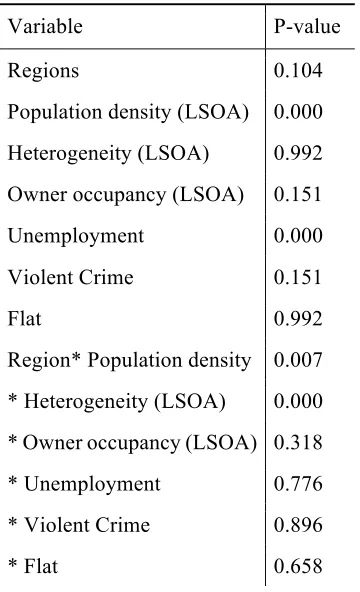
There is clear evidence of spatial patterning in survey response behaviour. Table 1 shows that including regional dummies significantly improves the fit compared with a global model that assumes no geographic effect. Survey response propensity varies by region after controlling for other important neighbourhood and household characteristics. Comparing the fit of Models 2 and 3 we see further that there is a significant interaction between region and at least some of the other predictors i.e. the effect of these predictors on response propensity varies by region.
Table 1: Fit comparison: Global vs. Regional Models
Degrees of freedom
Residual deviance
Deviance (Model 1 vs Model 2)
Deviance (Model 2 vs Model 3)
p-value
Model 1 4103 5638.3
Model 2 4092 5620.7 17.566
0.092
Model 3 4026 5500.6 120.08 0.000
Table 2: ANOVA for Model 3
Variable P-value
Regions 0.104
Population density (LSOA) 0.000
Heterogeneity (LSOA) 0.992
Owner occupancy (LSOA) 0.151
Unemployment 0.000
Violent Crime 0.151
Flat 0.992
Region* Population density 0.007
* Heterogeneity (LSOA) 0.000
* Owner occupancy (LSOA) 0.318
* Unemployment 0.776
* Violent Crime 0.896
* Flat 0.658
4.2.Geographically weighted regression
We can examine this geographic variation more fully using geographically weighted regression (GWR). Here we present the bivariate results from GWR. We will analyse separately the results for population density and heterogeneity as these were the two most significant variables in Model 3 above. We will conduct further analysis using multivariate GWR models.
4.2.1. Results for population density
There is variation in the estimated coefficients for population density ranging from positive to negative. A summary of the coefficients is shown in a Table 3. The distribution of the coefficients would suggest that the relationship between population density and survey response is not globally uniform.
Table 3 Summary of GWR coefficients for population density
n= 4255, bandwidth = 381, effective degrees of freedom = 4186.461, AIC = 2872.908
Minimum 1st quartile Median 3rd quartile Maximun
-0.0223 -0.00887 -0.00239 0.00241 0.0223
Figure 1 and 2 On the left the coefficients for population density estimated with GWR, on the right standard errors for the estimates
4.2.2. Results for heterogeneity
There is considerable variation in the heterogeneity coefficients as shown in Table 4. Coefficients for heterogeneity vary from positive to negative suggesting that the relationship between survey response and heterogeneity changes direction depending on the geographical location.
Table 4 Summary of GWR coefficients for heterogeneity
n= 4255, bandwidth = 461, effective degrees of freedom = 4197.823, AIC = 2881.441
Minimum 1st quartile Median 3rd quartile Maximun
-3.283 -0.8007 0.2269 1.495 10.77
The coefficients and standard errors for heterogeneity are presented in their geographical locations in Figures 3 and 4. Figure 3 confirms our previous finding that level of heterogeneity does not have a single global effect on survey response. The highest positive coefficients for heterogeneity are located in Northern Ireland whilst the strongest negative coefficients are found in the West Midlands and in London. This would suggest that the relationship between heterogeneity and response propensity is negative in more urban, ethnically heterogeneous areas of the UK.
Figure 3 and 4 On the left the coefficients for heterogeneity estimated with GWR, on the right standard errors for the estimates
5. Discussion
Our analysis demonstrates that there is a spatial dimension to survey response behaviour. Relying on a “one size fits all” model of response propensity for the whole of the UK is likely to be insufficient. Accommodating geography as a discrete entity defined by regional or other administrative boundaries is an improvement but still fails to capture the full picture. Using GWR toprovide a fuller account of spatial variation in survey response behaviour may improve our ability to both predict and explain response propensity across the UK. This in turn would enable survey practitioners to tailor fieldwork strategies more effectively and improve the quality of survey data collected and available for analysis. A further research task is to investigate effective ways to visualise multivariate GWR results allowing the comparison and exploration of different models
6. Acknowledgements
This work is part of the ‘Auxiliary Data Driven Nonresponse Bias Analysis (ADDReponse)’ project funded by the UK Economic and Social Research Council (grant ES/L013118/1).
7. Biography
Kaisa Lahtinen is a PhD student in University of Liverpool (as of 01.02.2016). She worked as a research officer in the ADDResponse project. She has interest in survey research and utilising new data sources.
Chris Brunsdon is Professor of Geocomputation and Director of the National Centrre for Geocomputation at Maynooth University, Ireland. He was one of the developers of GWR and has interests in analysing social data relating to crime, health, migration and other related topics.
References
Brunsdon, C., Fotheringham, S., Charlton, M., 1998. Geographically weighted regression. J. R. Stat. Soc. Ser. Stat. 47, 431–443.
Groves, R.M., 2006. Nonresponse Rates and Nonresponse Bias in Household Surveys. Public Opin. Q. 70, 646–675. doi:10.1093/poq/nfl033
Groves, R.M., Couper, M., 1998. Nonresponse in household interview surveys, Wiley series in probability and statistics. Wiley, Chichester.
Johnson, T.P., Cho, Y.I., Campbell, R.T., Holbrook, A.L., 2006. Using Community-Level Correlates to Evaluate Nonresponse Effects in a Telephone Survey. Public Opin. Q. 70, 704–719. doi:10.1093/poq/nfl032
Massey, D.S., Tourangeau, R., 2013. Where Do We Go from Here? Nonresponse and Social Measurement. Ann. Am. Acad. Pol. Soc. Sci. 645, 222–236. doi:10.1177/0002716212464191 Stoop, I.A.L. (Ed.), 2010. Improving survey response: lessons learned from the European Social