Numerical techniques on improving computational efficiency of spectral boundary integral method

City, University of London Institutional Repository

Citation

:

This is the accepted version of the paper.

This version of the publication may differ from the final published

version.

Permanent repository link:

Link to published version

:

Copyright and reuse:

City Research Online aims to make research

outputs of City, University of London available to a wider audience.

Copyright and Moral Rights remain with the author(s) and/or copyright

holders. URLs from City Research Online may be freely distributed and

linked to.

City Research Online: http://openaccess.city.ac.uk/ [email protected]

Peer Review Only

Numerical techniques on improving computational efficiency

of Spectral Boundary Integral Method

Jinghua Wang and Q.W. Ma*

School of Engineering and Mathematical Sciences, City University London, United Kingdom *Corresponding Author Email: [email protected]

SUMMARY

Numerical techniques are suggested in this paper, in order to improve the computational efficiency of the Spectral Boundary Integral Method, initiated by Clamond & Grue [D. Clamond and J. Grue. A fast method for fully nonlinear water-wave computations. J. Fluid Mech. 2001; 447: 337-355] for simulating nonlinear water waves. This method involves dealing with the high order convolutions by using Fourier Transform or Inverse Fourier Transform and evaluating the integrals with weakly singular integrands. A de-singularity technique is proposed here to help efficiently evaluating the integrals with weak singularity. An anti-aliasing technique is developed in this paper to overcome the aliasing problem associated with Fourier Transform or Inverse Fourier Transform with a limited resolution. This paper also presents a technique for determining a critical value of the free surface, under which the integrals can be neglected. Numerical tests are carried out on the numerical techniques and on the improved method equipped with the techniques. The tests will demonstrate that the improved method can significantly accelerate the computation, in particular when waves are strongly nonlinear.

KEYWORDS: nonlinear water waves; boundary integral method; de-singularity technique; anti-aliasing technique; spectral method

1. INTRODUCTION

Peer Review Only

opened another door for studying nonlinear water waves.

Fully nonlinear analysis did not start until the emerging of advanced computing technologies. The Boundary Element Method (BEM) was first introduced by Longuet-Higgins & Cokelet [18], who started a new era to model the fully nonlinear waves numerically. It was successfully applied to simulate two-dimensional (2D) overturning waves. The algorithm of BEM was later improved by Grilli et al. [19], Dold [20] and many others. Meanwhile, Wu & Eatock-Taylor [22, 23] proposed the Finite Element Method (FEM) to study the interaction between water waves and structures. This method was later extended to 3D cases by Ma [24] and Ma et al. [25, 26]. More recently, Yan & Ma [28, 29] and Ma & Yan [27, 30] introduced a new mesh strategy and proposed the Quasi Arbitrary Lagrangian-Eulerian Finite Element Method (QALE-FEM). The results obtained by using this method for 2D and 3D overturning and other strong nonlinear waves are impressive. On the other hand, Dommermuth & Yue [31] developed a tool, known as the Higher-Order Spectral Method (HOS), which was able to model waves effectively with the help of Fast Fourier Transform (FFT). However, this method was built on the assumption that the Taylor expansion of the velocity potential at the free surface was convergent. Due to this, the method does not work well when the waves are quite steep [31]. Nicholls [32] proposed a numerical model called Spectral Continuation Method to study the traveling water waves. In this method, the Dirichlet-Neumann operator was approximated by an assumed analytic function of the free surface elevation and was expanded into Taylor series. Due to the fact that the evaluation of the higher order terms is highly recursive and impractical, they chose to only use the 5th order in practice. As a consequence, this method is incapable to capture the higher order nonlinearities. Clamond & Grue [1] proposed a novel method based on a boundary integral method and FFT. Fructus et al. [4] made one step further extending this method to 3D cases. The method has been summarized by Grue & Fructus [40]. In this method, the Neumann operator was introduced and expressed in terms of the free surface and the velocity potential. The kinematic and dynamic boundary conditions were reformulated into the skew-symmetric form after applying the Fourier transform. The free surface and velocity potential are updated through integrating the equations with respect to time, which requires the velocity on the free surface. The velocity on the free surface is decomposed into convolution parts (to 3rd order in [4]) and integration parts. Convolution parts are evaluated by FFT, and the integration parts have kernels decaying quickly along the distance between the source and field points but their integrands are weakly singular. The property of the kernels enables the local integration to be estimated within a limited range (e.g., two characteristic wave lengths, say 𝑋 − 𝐿0 to 𝑋 + 𝐿0), instead of (−∞, ∞). Even though the integration

Peer Review Only

addressed to make the method more robust and efficient:

a) Weak singularity in the integrals requires to be dealt with carefully. Fructus et al. [4] have proposed a method for this. They suggested that the weak

singularity was eliminated by evaluating the integrals at a shifted point 𝑿 +

1

2∆𝑿, rather than at the singular point. This method was found to give good

results when the grids used are sufficiently fine. However, fine grids require relatively long computational time. Ideally, the similar results can be obtained by using relatively coarse grids.

b) Though the solutions for removing aliasing problems involved in the convolutions up to the 4th order have been proposed by Fructus et al. [4], it is found that the method did not work well for the convolutions of 5th or higher order. However, the technique of removing aliasing problems for higher-order convolutions was not proposed yet.

c) When the boundary integrals are evaluated with the convolutions up to the 7th

order and the integration parts are neglected as suggested by Grue [3], one needs to know the critical value of the free surface gradient, under which the approach with neglecting integration parts can give sufficiently accurate results but cannot do so beyond this. The critical free surface gradient deserves a study which has not been carried out yet.

This paper will present the numerical techniques to address the above issues. With these technique, the method described in [1-4] becomes more computational efficient and more robust. For convenience, the method described in [1-4] is named as Spectral Boundary Integral Method in this paper.

2. MATHEMATICAL FORMULATIONS

2.1. The prognostic equation

The fully nonlinear potential theory requires the kinematic and dynamic boundary conditions at the free surface to be satisfied. In the dimensionless form [31], they are

𝜕𝜂 𝜕𝑇 =

𝜕𝜙

𝜕𝑍− ∇𝜙 ∙ ∇𝜂 (1)

𝜕𝜙 𝜕𝑇+ 𝜂 +

1

2(∇𝜙 ∙ ∇𝜙 + 𝜕𝜙 𝜕𝑍

2

) + 𝑝 = 0 (2)

where ∇=_𝜕𝑿𝜕 =_𝜕𝑋𝜕 𝑖⃗ +_𝜕𝑌𝜕 𝑗⃗ is the horizontal gradient operator, and 𝜂 is the elevation

of the free surface, 𝜙 is the velocity potential, 𝑝 is the pressure on the free surface and 𝑝 = 0 if it is not specified. Among the variables in the equations above, 𝜂, 𝑿 and 𝑍 have been non-dimensionalized by multiplying 𝐾₀, 𝜙 by multiplying

√𝐾₀3_{/𝑔, 𝑝 by multiplying 𝐾}

0/(𝜌𝑔), and 𝑇 by multiplying Ω0. 𝐾0 is the

Peer Review Only

𝜌 the density of the fluid and 𝑔 the gravity acceleration. The wave number of the most energetic component in the spectrum at the beginning of the simulation is chosen as the characteristic wave number 𝐾0. After introducing the new variable in

Neumann form representing the vertical velocity, 𝑉 = 𝜕𝜙_𝜕𝑛√1 + |∇𝜂|2, where 𝑛 is

the normal vector of the free surface, Equation (1) and (2) become

𝜕𝜂

𝜕𝑇− 𝑉 = 0 (3)

𝜕𝜙̃ 𝜕𝑇+ 𝜂 +

1 2(|∇𝜙̃|

2

−(𝑉 + ∇𝜂 ∙ ∇𝜙̃)

2

1 + |∇𝜂|2 ) + 𝑝 = 0 (4)

where 𝜙̃ denotes the velocity potential on the free surface 𝜙̃(𝑿, 𝑇) = 𝜙(𝑿, 𝑍 =

𝜂(𝑿, 𝑇), 𝑇). One should note that derivatives of 𝜙̃ in Equation (3) & (4) are different from these of 𝜙 in Equations (1) & (2). They satisfy the relation

∇𝜙̃ = (∇𝜙)|𝑍=𝜂+ (

𝜕𝜙

𝜕𝑍)|_𝑍=𝜂∇𝜂 (5)

𝜕𝜙̃ 𝜕𝑇 = (

𝜕𝜙

𝜕𝑇)|𝑍=𝜂 + (

𝜕𝜙 𝜕𝑍)|𝑍=𝜂

𝜕𝜂

𝜕𝑇 (6)

Following [4], the Fourier transform and the inverse Fourier transform are defined as (take the velocity potential on the free surface for example)

𝜙̂(𝑲, 𝑇) = 𝐹{𝜙̃} = ∫ 𝜙̃(𝑿, 𝑇)𝑒−𝑖𝑲∙𝑿_𝑑𝑿 𝑆0

𝜙̃(𝑿, 𝑇) = 𝐹−1_{{𝜙̂} =} 1

4𝜋2∫ 𝜙̂(𝑲, 𝑇)𝑒𝑖𝑲∙𝑿𝑑𝑲 𝑆0

(7)

where 𝑲 is the wave number and 𝑆₀ is the projection of the whole free surface on the horizontal plane. After applying Fourier transform, Equations (3) & (4) lead to the following skew-symmetric prognostic equation

𝜕𝑀⃗⃗⃗

𝜕𝑇 + 𝐴𝑀⃗⃗⃗ + 𝑅⃗⃗ = 𝑁⃗⃗⃗ (8)

where

𝑀⃗⃗⃗ = ( 𝐾𝐹{𝜂}

𝐾Ω𝐹{𝜙̃}), 𝐴 = [0 −ΩΩ 0 ], 𝑅⃗⃗ = ( 0

𝐾Ω𝐹{𝑝}), 𝑁⃗⃗⃗ =

(_{𝐾Ω𝐹{𝐺}𝐾𝐹{𝐺1}

2})

𝐹{𝐺1} = 𝐹{𝑉} − 𝐾𝐹{𝜙̃}

𝐹{𝐺2} = 𝐹 {

1 2[

(𝑉 + ∇𝜂 ∙ ∇𝜙̃)2

1 + |∇𝜂|2 − |∇𝜙̃| 2

]}

Peer Review Only

and 𝛺 = √𝐾, 𝐾 = |𝑲|. The solution to Equation (8) is given as

𝑀⃗⃗⃗(𝑇) = 𝑒−𝐴(𝑇−𝑇0)∫ 𝑒𝐴(𝑇−𝑇0)(𝑁⃗⃗⃗ − 𝑅⃗⃗)𝑑𝑇

𝑇

𝑇0

+ 𝑒−𝐴(𝑇−𝑇0)𝑀⃗⃗⃗(𝑇₀) ₍₁₀₎

where

𝑒𝐴∆𝑇 _{= [cos Ω∆}𝑇 − sin Ω∆𝑇

sin Ω∆𝑇 cos Ω∆𝑇 ] (11)

According to Clamond and Fructus [33], this time integrator is linearly stable and exact. The six-stage embedded 5th _{order Runge-Kutta method is adopted to solve the}

equation numerically. The solution can be written as

𝑀⃗⃗⃗(4) = 𝑒−𝐴(𝑇−𝑇0)[𝑀⃗⃗⃗(𝑇₀) + ∑ 𝛼_𝑖𝜅_𝑖

6

𝑖=1

]

𝑀⃗⃗⃗(5)_{= 𝑒}−𝐴(𝑇−𝑇0)[𝑀⃗⃗⃗(𝑇₀) + ∑ 𝛽_𝑖𝜅_𝑖

6

𝑖=1

]

(12)

where coefficients 𝛼𝑖 and 𝛽𝑖 can be found in [34], and 𝜅𝑖 is the Runge-Kutta

increment at each stage. The superscripts (4) and (5) represent the 4th order and 5th order solution of the Runge-Kutta time integrator respectively. The time step size is self-adaptive which is determined by imposing the following condition

𝐸𝑟𝑟𝑇 = ∫[|𝜂

(5)_{− 𝜂}(4)_{| + |𝜙̃}(5)_{− 𝜙̃}(4)_{|] 𝑑𝑿}

∫[|𝜂(5)_{| + |𝜙̃}(5)_|]𝑑𝑿 < 𝑇𝑜𝑙𝑇 (13)

where 𝐸𝑟𝑟_𝑇 is the relative error between the 4th _{and 5}th _{order solutions and 𝑇𝑜𝑙}

𝑇 is

the tolerance. Using the equation, one can obtain the optimised time step size ∆𝑇_𝑜𝑝𝑡 as a function of 𝐸𝑟𝑟_𝑇, as suggested in [33].

2.2. The boundary integral solver

One can find the solutions from Equation (10) for the wave elevation (𝜂) and velocity potential (𝜙̃) on the free surface if the velocity 𝑉 on the free surface is given. To obtain 𝑉, one needs to solve the Laplace equation governing the velocity potential in the whole fluid domain, which can be transferred to a boundary integral equation using the Green’s theorem. The procedure and methodology is well known and so details will not be given here. Only the result of the boundary integral equation in [18] is written out as follows for completeness,

∬ 1

𝑟 𝜕𝜙′ 𝜕𝑛′

𝑆

𝑑𝑆′ = 2𝜋𝜙̃ + ∬ 𝜙̃′ 𝜕 𝜕𝑛′

1 𝑟

𝑆

𝑑𝑆′ (14)

where S is the area of the instantaneous free surface, the variables with the prime indicate those at source point (𝑿′, 𝑍′), the variables without the prime are those at

field point (𝑿, 𝑍), 𝑟 = √𝑅2+ (𝑍′− 𝑍)2 and 𝑅 = |𝑹| = |𝑿′− 𝑿|, 𝑆′ denotes the

Peer Review Only

as

∫ 𝑉′ 𝑟 𝑑𝑿′

𝑆0

= 2𝜋𝜙̃ + ∫ 𝜙̃′√1 + |∇′𝜂′|2 𝜕

𝜕𝑛′ 1 𝑟𝑑𝑿′

𝑆0

(15)

where 𝑆₀ is the projection of 𝑆′ on to the horizontal plane, which is the same as in

Equation (7). After introducing a new variable 𝐷 =𝜂 ′_−𝜂

𝑅 , the above equation becomes

(details could be found in [1, 4])

∫ 𝑉′ 𝑅 𝑑𝑿′

𝑆0

= 2𝜋𝜙̃ + ∫ (𝜂′_{− 𝜂)∇}′_{𝜙̃′ ∙ ∇}′1

𝑅𝑑𝑿′

𝑆0

− ∫ 𝜙̃′_[ 1

(1 + 𝐷2₎3/2− 1] ∇′∙ [(𝜂′− 𝜂)∇′

1 𝑅] 𝑑𝑿′

𝑆0

− ∫ 𝑉′ 𝑅 (

1

√1 + 𝐷2− 1) 𝑑𝑿 ′ 𝑆0

(16)

The velocity 𝑉 can be split into four parts, i.e., 𝑉 = 𝑉1+ 𝑉2+ 𝑉3+ 𝑉4. Each part is

given by

𝑉₁ = 𝐹−1_{{𝐾𝐹{𝜙̃}} (17)}

𝑉₂ = −𝐹−1_{{𝐾𝐹{𝜂𝑉}

1}} − ∇ ∙ (𝜂∇𝜙̃) (18)

𝑉3 = 𝑉3,𝐼′ = 𝐹−1{

𝐾

2𝜋𝐹 {∫ 𝜙̃′∇′∙ [(𝜂′− 𝜂)∇′ 1

𝑅] Γ1(D)𝑑𝑿′

𝑆0

}}

= 𝐹−1_{𝐾

2𝜋𝐹 {∫ 𝜙̃′

(𝜂′_{− 𝜂) − 𝑹 ∙ ∇}′_𝜂′

𝑅3 Γ1(D)𝑑𝑿′ 𝑆0

}}

(19)

𝑉₄ = 𝐹−1_{𝐾

2𝜋𝐹 {∫ 𝑉′

𝑅 (1 − 1

√1 + 𝐷2) 𝑑𝑿 ′ 𝑆0

}} (20)

where

Γ₁(D) = 1 − 1

(1 + 𝐷2₎3/2 (21)

Fructus et al. [4] had expanded the expression of 𝑉₄ to the 3rd order convolutions, plus a remaining integration term, that is

𝑉₄ = 𝑉₄(1)+ 𝑉_4,𝐼′

= 𝐹−1_{−𝐾

2[𝐾𝐹{𝜂2𝑉} − 2𝐹 {𝜂𝐹−1{𝐾𝐹{𝜂𝑉}}} + 𝐹 {𝜂2𝐹−1{𝐾𝐹{𝑉}}}]}

+𝐹−1_{𝐾

2𝜋𝐹 {∫ 𝑉′

𝑅 Υ1(𝐷)𝑑𝑿′}}

Peer Review Only

where

Υ1(𝐷) = 1 −

1 √1 + 𝐷2 −

1

2𝐷2 (23)

𝑉₄(1) denotes the 3rd order convolutions in the first curly-bracket term and 𝑉_4,𝐼′

represents the remaining integration part in the second curly-bracket term on the right of Equation (22). Note that the determination of 𝑉₁, 𝑉₂ and 𝑉₃ is explicit while the determination of 𝑉4 is implicit and needs iterations.

During iteration for finding 𝑉₄, the initial value of 𝑉₄ is firstly estimated by letting

𝑉 = 𝑉1+ 𝑉2 and assuming

𝐸𝑟𝑟𝐵 =∫|𝑉

𝐼𝑡𝑒𝑟_{− 𝑉}𝐼𝑡𝑒𝑟+1_|𝑑𝑿

∫|𝑉𝐼𝑡𝑒𝑟+1_|𝑑𝑿 < 𝑇𝑜𝑙𝐵 (24)

with 𝑉𝐼𝑡𝑒𝑟 and 𝑉𝐼𝑡𝑒𝑟+1 being the values of the velocity 𝑉 at the two successive iterations.

It is noted here that based on the definition of 𝐷 =𝜂 ′_−𝜂

𝑅 , one obtains that 𝐷 →

𝜕𝜂/𝜕𝑅 or |𝐷| → |∇𝜂| if 𝑅 → 0. Thus 𝐷 represents the local gradient of waves or wave steepness and reflects their nonlinearity. The maximum of 𝐷 is determined by

|𝐷|𝑚𝑎𝑥 = |𝜕𝜂/𝜕𝑅 |𝑚𝑎𝑥, where |𝜕𝜂/𝜕𝑅 |𝑚𝑎𝑥 is the maximum gradient of the free

surface in the spatial domain and may change with time.

2.3. Numerical implementation

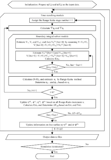
Based on the descriptions in [1, 2, 4], we draw out the flow chart in Figure 1 to illustrate the whole numerical scheme and procedure of the spectral boundary integral method. In this figure, the gradient of the free surface ∇𝜂 and the velocity potential

∇𝜙̃ are estimated by Fourier and its inverse transform

∇𝜂 = 𝐹−1_{{𝑖𝑲𝐹{𝜂}} 𝑎𝑛𝑑 ∇𝜙̃ = 𝐹}−1_{{𝑖𝑲𝐹{𝜙̃}} (25)}

Peer Review Only

Figure 1. Flow chart for the numerical implementation of Spectral Boundary Integral Method

2.4. Schemes for estimating 𝑉3 and 𝑉4

Fructus et al. [4] had expanded the expression of 𝑉₄, and replaced the main part with convolutions to the 3rd order as indicated above. Grue [3] brought the expressions of both 𝑉₃ and 𝑉₄ to convolutions of the 6th and 7th order respectively. We repeat the expanding procedures and have obtained the equivalent but slightly different results, given by (refer to appendix for details)

𝑉₃ = 𝑉_3,𝐶+ 𝑉_3,𝐼 = 𝑉_⏟3(1)

4𝑡ℎ

+𝑉_⏟3(2)

6𝑡ℎ

+ 𝑉_⏟3,𝐼

Peer Review Only

3𝑟𝑑

+ 𝑉_⏟4(2)

5𝑡ℎ

+ 𝑉_⏟4(3)

7𝑡ℎ

+ 𝑉_⏟4,𝐼

𝑖𝑛𝑡𝑒𝑔𝑟𝑎𝑡𝑖𝑜𝑛 (27)

𝑉_3,𝐼 = 𝐹−1_{𝐾

2𝜋𝐹 {∫ 𝜙̃′

(𝜂′_{− 𝜂) − 𝑹 ∙ ∇}′_𝜂′

𝑅3 Γ2(D)𝑑𝑿′}} (28)

𝑉4,𝐼 = 𝐹−1{

𝐾 2𝜋𝐹 {∫

𝑉′

𝑅 Υ2(𝐷)𝑑𝑿′}} (29)

where

Γ2(D) = 1 −

1

(1 + 𝐷2₎3/2−

3 2𝐷2+

15

8 𝐷4 (30)

Υ₂(𝐷) = 1 − 1 √1 + 𝐷2−

1 2𝐷2 +

3 8𝐷4−

5

16𝐷6 (31)

𝑉_3,𝐶 = 𝑉₃(1)+ 𝑉₃(2) and 𝑉_4,𝐶 = 𝑉₄(1)+ 𝑉₄(2)+ 𝑉₄(3) are convolution parts and the

order of each convolution is labelled at the bottom of each term. The order of the convolution is defined in this way, for example, 𝐹{𝑉𝜂𝐼−1}~𝑂(𝜀𝐼), as the 𝐼𝑡ℎ order, where 𝜀 = 𝐾0𝐴 is the characteristic wave steepness and 𝐴 is the wave amplitude.

When the steepness is small, the order of the integration parts 𝑉_3,𝐼 and 𝑉_4,𝐼 are insignificant compared with the convolution parts, and so can be neglected. Generally, three approaches of estimating 𝑉₃ and 𝑉₄ are suggested, as summarized in Table I.

Table I. Schemes of the boundary integral solver

Scheme 1 𝑉3 = 𝑉3,𝐼′ 𝑉₄ = 𝑉₄(1)+ 𝑉_4,𝐼′

Scheme 2 𝑉3= 𝑉3,𝐶 𝑉4 = 𝑉4,𝐶

Scheme 3 𝑉₃ = 𝑉_3,𝐶+𝑉_3,𝐼 𝑉₄ = 𝑉_4,𝐶+ 𝑉_4,𝐼

In Scheme 1, 𝑉₃ is estimated with integration. 𝑉₄ is expanded to 3rd order convolution plus integration term. In Scheme 2, 𝑉₃ and 𝑉₄ are expanded to the 6th

and 7th _{order convolutions respectively, but ignoring both 𝑉}

3,𝐼 and 𝑉4,𝐼. Scheme 3 is

the same as Scheme 2, except the integration parts are included.

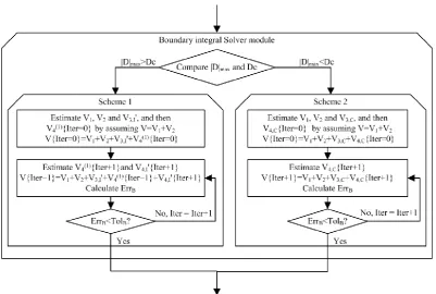
It is understood that Scheme 1 and Scheme 3 are equivalent. However, Scheme 3 requires more computational efforts over Scheme 1 on calculating the convolution parts, thus this scheme is only used as benchmark to quantify the difference between Scheme 1 and Scheme 2. In addition, Scheme 2 is the most efficient but is only valid when 𝐷 is not too big. Assume there exist a critical value 𝐷_𝑐, under which the velocity can be solved by Scheme 2; otherwise by Scheme 1, the boundary integral solver module in Figure 1 can be replaced by the flow chart in Figure 2.

Peer Review Only

In addition, Fructus et al. [4] applied Scheme 1 to Stokes waves while Grue [3] employed Scheme 2 to simulate 3D wave fields, as indicated above. One of main contributions of this paper is to suggest mixing the two schemes together and more importantly to develop a technique for quantitatively determining the critical value

𝐷𝑐, so that the computation can automatically switch to Scheme 1 or Scheme 2

according to the instantaneous value of |𝐷|𝑚𝑎𝑥, significantly accelerating the

computation of wave fields. The details about this will be presented in the later section below.

Figure 2. The flow chart of the numerical scheme for solving the boundary integral equation

3. DE-SINGULARITY TECHNIQUE

As mentioned in previous section, the integrals in Equations (19), (22), (28) and (29) have weak singular integrands. Such singularity is an inherited problem for all methods based on the boundary integrals dealing with gravity water waves, from when they were introduced by Longuet-Higgins & Cokelet [18] in their study on the 2D overturning waves. In their paper, the normal velocity 𝜙_𝑛 appeared in

∫ 𝜙𝑛ln 𝑠 𝑑𝑠, where 𝑠 is the arc-length on the boundary, was expanded at 𝑠 = 0 and

𝑠𝑖_{ln 𝑠 was integrated analytically. Grilli et al. [19] dealt with the singular integrals by}

using so called ‘singularity extraction’ method for their normal boundary element method applying to 3D wave problems. In the approach, they introduced the polar coordinates and then transformed the principle integration to a regular integration.

For the Spectral Boundary Integral Method, Fructus et al. [4] suggested evaluating

the integrands at nodes 𝑿 +1₂∆𝑿, and shifting back to regular nodes through Fourier

Peer Review Only

considering the elements around the singular points so that the contributions to the integration coming from this area are neglected. The smaller of the neglected area is, the more accurate the numerical integration is. In other words, to achieve high accuracy of results, the number of elements splitting the free surface has to be large. This can decelerate the computational process. In this paper, an alternative technique is suggested to evaluate the singular integrals for the the spectral boundary integral method.

3.1. Weakly singular integral in 𝑉₄

Similar to the strategy by Grilli et al. [19], we re-write the integration part of 𝑉₄ around the singular point as

lim

𝜎→0∫

𝑉′_Υ 𝑖

𝑅 𝑑𝑿′

𝑆−𝜎

= lim

𝜎→0∫

𝑓̃(𝑿′₎

𝑅 𝑑𝑿′

𝑆−𝜎

(32)

where Υ_𝑖 is given by Equation (23) or (31), 𝜎 is an area surrounding the singular point. Using the local polar coordinates illustrated in Figure 3, the right hand side of Equation (32) can be rewritten as

lim

𝜎→0∫

𝑓̃(𝑿′₎

𝑅 𝑑𝑿′

𝑆−𝜎

= lim

𝛿→0∫ ∫ 𝑓(𝑅, 𝜃)𝑑𝑅𝑑𝜃 𝜌(𝜃)

𝛿 2𝜋

0

= ∫ ∫ 𝑓(𝑅, 𝜃)𝑑𝑅𝑑𝜃

𝜌(𝜃)

0 2𝜋

0

(33)

where 𝜌(𝜃) and 𝛿 are the radius of the area 𝑆 and 𝜎 respectively, and

𝑓̃(𝑿′_{) = 𝑓(𝑅, 𝜃) = 𝑉′Υ}

𝑖 (34)

with 𝐷 →𝜕𝜂_𝜕𝑋𝑐𝑜𝑠𝜃 +𝜕𝜂_𝜕𝑌𝑠𝑖𝑛𝜃 for 𝑅 → 0. The expression in Equation (34) is not

Peer Review Only

Figure 3. The local polar coordinates for the elements near the singular point

3.2. Weakly singular integral in 𝑉₃

Following the same strategy, this weakly singular integral around the singular point in the expression of 𝑉₃ is written as

lim

𝜎→0∫

𝑔̃(𝑿′₎

𝑅2 𝑑𝑿′ 𝑆−𝜎

= lim

𝜎→0∫

𝑔(𝑅, 𝜃) 𝑅 𝑑𝑅𝑑𝜃

𝑆−𝜎

(35)

where

𝑔(𝑅, 𝜃) = 𝑔̃(𝑿′_{) = 𝜙̃}′_{(𝐷 −}𝑹 ∙ ∇′𝜂′

𝑅 ) Γi (36)

and Γi is defined by Equation (21) or (30). Note that lim_𝑅→0(𝑹∙∇

′_𝜂′

𝑅 − 𝐷)= 0, which

means 𝑔(𝑅 = 0, 𝜃) = 0. Thus, in order to evaluate the integral numerically, we approximate 𝑔(𝑅, 𝜃) with the first order Taylor series

𝑔(𝑅, 𝜃) = 𝑔(0, 𝜃) +𝜕𝑔

𝜕𝑅(0, 𝜃)𝑅 + O(𝑅2) (37)

Then we have

∫ ∫ 𝑔(𝑅, 𝜃) 𝑅 𝑑𝑅𝑑𝜃

𝜌(𝜃)

0 2𝜋

0

= ∫ ∫ 𝜕𝑔

𝜕𝑅(0, 𝜃)𝑑𝑅𝑑𝜃

𝜌(𝜃)

0 2𝜋

0

= ∫ 𝑔(𝑅 = 𝜌, 𝜃)𝑑𝜃

2𝜋 0

(38)

which provides a solution for converting the weakly singular integration to a regular

Peer Review Only

approximation to 𝑔(𝑅, 𝜃) has been used so that the integration with respect to 𝑅 leads to 𝑔(𝑅 = 𝜌, 𝜃). The last integral in Eq. (38) is estimated by using one dimensional trapezium rule.

3.3. Effectiveness of the de-singular techniques for evaluating 𝑉₃ and 𝑉₄ In order to show how effective the above de-singular techniques are, the cases for Stokes waves presented in [4] are tested in this section. To model the case, the initial free surface elevation and velocity potential on the free surface are calculated by using the Fenton’s numerical solver [35] up to 7th order with the wave steepness of

𝜀 = 𝜋𝐻/𝐿 = 0.2985 (𝐻 is the wave height and 𝐿 = 2𝜋 is the wave length) in a spatial domain of 2𝐿 × 2𝐿. In addition, our numerical tests indicate that any value of

𝑇𝑜𝑙_𝐵 ≤ 1𝐸 − 5 in Equation (24) leads to almost the same results and so the value of

𝑇𝑜𝑙𝐵 is taken as 1𝐸 − 5 hereafter.

The specific values of 𝑉₃ and 𝑉₄ are time-dependent. We will first examine the effectiveness of the de-singularity technique using the profiles of 𝑉₃ and 𝑉₄ at the first time step. These profiles obtained by the methods with or without the de-singularity technique are shown in Figure 4 for different numbers of elements represented by the resolution. The profiles are normalized by 𝑉30 and 𝑉40, which are

the maxima of 𝑉₃ and 𝑉₄ corresponding to the resolution 210*210. The results for the case without the de-singularity technique are obtained by using the same method as in [4], that is, the singularity is avoided by evaluating the integrands of 𝑉3 and 𝑉4 at a

shifted point (𝑿 +1

2∆𝑿). As the de-singularity techniques are relevant only to the

integration parts in 𝑉₃ and 𝑉₄, the results plotted are only these parts in 𝑉₃ and 𝑉₄. As can be seen from Figure 4, without the de-singularity technique, the peak values of both 𝑉₃ and 𝑉₄ are significantly under-estimated when the resolution is not sufficiently high. With increase of the resolution, the profiles of 𝑉₃ and 𝑉₄ gradually coincide with each other. Specifically, at the resolution of 29*29, the difference between them becomes negligible. This demonstrates that the approach proposed in [4] can give accurate results but requires higher resolution. In order to shed more light on the performance of the techniques, their errors are analyzed using the following equations

𝐸𝑟𝑟𝑜𝑟{𝑉3} =

∫ |𝑉3− 𝑉3 (𝑁=210₎

| 𝑑𝑋

∫ |𝑉₃(𝑁=210)| 𝑑𝑋

𝐸𝑟𝑟𝑜𝑟{𝑉₄} =∫ |𝑉4− 𝑉4

(𝑁=210)_{| 𝑑𝑋}

∫ |𝑉₄(𝑁=210)| 𝑑𝑋

(39)

where 𝑉₃(𝑁=2 10₎

and 𝑉₄(𝑁=210) are the values of 𝑉₃ and 𝑉₄ calculated using

Peer Review Only

technique for the resolution of 26*26 is as small as that obtained without the de-singularity technique for the resolution of 210*210, while the error from the method without the de-singularity technique for the resolution of 26*26 is more than 6 times larger than the latter. This further demonstrates that the de-singularity technique help achieving the similar results with much low resolution or achieving the results with higher accuracy by using the same resolution, compared to the approach suggested in [4], which also leads to exact results but with relatively slower convergent rate.

0 0.5 1 1.5 2

-1.5 -1 -0.5 0 0.5 1 1.5 X/L V3 / V 30

Resolution: 26*26

0 0.5 1 1.5 2

-1.5 -1 -0.5 0 0.5 1 1.5 X/L V4 / V 40

Resolution: 26*26

0 0.5 1 1.5 2

-1.5 -1 -0.5 0 0.5 1 1.5 X/L V 3 / V 30

Resolution: 27*27

0 0.5 1 1.5 2

-1.5 -1 -0.5 0 0.5 1 1.5 X/L V4 / V 40

Resolution: 27*27

0 0.5 1 1.5 2

-1.5 -1 -0.5 0 0.5 1 1.5 X/L V3 / V 30

Resolution: 28*28

0 0.5 1 1.5 2

-1.5 -1 -0.5 0 0.5 1 1.5 X/L V4 / V 40

Peer Review Only

Figure 4. Profiles of 𝑉₃ and 𝑉₄

Solid: with de-singularity technique; Dash: without de-singularity technique

(a) (b)

Figure 5. Relative error of the profiles of 𝑉3(a) and 𝑉4(b)

Solid: with de-singularity technique; Dash: without de-singularity technique

Next, the effects of the de-singularity technique on overall wave propagation of a long period will be examined. The same waves for Figure 4 and Figure 5 are considered but simulated in different sizes (2𝐿 × 2𝐿, 4𝐿 × 2𝐿 and 8𝐿 × 2𝐿) of the spatial domain. To simulate these cases, the resolution used is 26_*26_{, 2}7_*26 _{and 2}8_*26_,

(i.e., the number of elements per wave length is the same), respectively. The wave profiles after the simulation of 1000𝑇₀ (𝑇₀ is the wave period output by the Fenton’s numerical solver [35], which is 6.0095 in this case) are plotted in Figure 6. If there would be no error, the profiles after the propagation of 1000𝑇₀ should coincide

0 0.5 1 1.5 2

-1.5 -1 -0.5 0 0.5 1 1.5 X/L V3 / V 30

Resolution: 29*29

0 0.5 1 1.5 2

-1.5 -1 -0.5 0 0.5 1 1.5 X/L V4 / V 40

Resolution: 29*29

0 0.5 1 1.5 2

-1.5 -1 -0.5 0 0.5 1 1.5 X/L V3 / V 30

Resolution: 210*210

0 0.5 1 1.5 2

-1.5 -1 -0.5 0 0.5 1 1.5 X/L V4 / V 40

Resolution: 210*210

6 7 8 9 10

0 0.05 0.1 0.15 0.2 0.25 0.3 0.35

Resolution (2n)

E rr o r{ V 3 }

6 7 8 9 10

0 0.05 0.1 0.15 0.2

Resolution (2n)

Peer Review Only

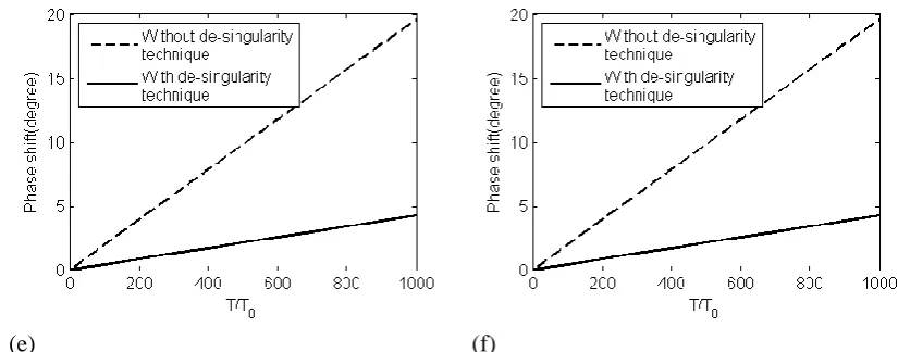
with the initial profile (the dotted line in the figure). One can see from this figure that the profile obtained without the de-singularity technique has a large phase shift (about 20 degree), while that obtained with the de-singularity technique has only a small phase shift (about 4 degree). The phase shift is gradually accumulated during the simulation. The variation of the phase shift with time is depicted in Figure 7 for different sizes of spatial domain. It clearly shows that the phase shift varies linearly with time and eventual values are almost the same for different domains. In addition, the effects of 𝑇𝑜𝑙𝑇 used in Equation (13) are also shown in this figure and in Table

II. All the information confirms that 𝑇𝑜𝑙_𝑇 = 1𝐸 − 7 is sufficiently small to give consistent results.

Table II. Phase shift with different experimental conditions Phase shift

(degree)

𝑇𝑜𝑙_𝑇= 1𝐸 − 6 𝑇𝑜𝑙_𝑇 = 1𝐸 − 7 𝑇𝑜𝑙_𝑇 = 1𝐸 − 8 o × √ o × √ o × √ 2𝐿 × 2𝐿 domain -56 19.52 4.33 16 19.60 4.26 18 19.61 4.25

4𝐿 × 2𝐿 domain - 19.56 4.29 - 19.60 4.25 - 19.61 4.25

8𝐿 × 2𝐿 domain - 19.58 4.26 - 19.61 4.25 - 19.61 4.25

Note: ‘o’ result from Fructus et al.[4]; ‘×’ without de-singularity technique; ‘√’ with

de-singularity technique

To further examine the effectiveness of the new de-singularity technique quantitatively, the errors defined in two different ways are introduced below:

a) The total phase shift error

𝐸𝑟𝑟₁ = 100|∆𝜑|

2𝜋 (40)

b) The mean phase shift error per wave period

𝐸𝑟𝑟2 =

𝐸𝑟𝑟₁

𝑁𝑡𝑜 (41)

where ∆𝜑 is the total phase shift in radians over the whole period of simulation and

𝑁𝑡𝑜 is the total number of wave periods of simulation, which is 1000 in this case.

The errors of the same case as in Figure 6(a) for the domain size of 2𝐿 × 2𝐿 but obtained using different resolutions are plotted in Figure 8(a), where the number of horizontal axis represents the power (n) of 2n (the same employed hereafter). In addition, the CPU time against different errors for running all the simulations up to

1000𝑇0 on a workstation equipped with the Intel Xeon E5-2630 v2 of 2.6GHz

Peer Review Only

The ratio of the minimum resolutions and corresponding CPU time needed to achieve the error less than 2.5% by the methods with and without use of the de-singularity technique are shown in Figure 9. The ratio in this figure is calculated in the way that the value of the method without the de-singularity technique is divided by that of the method with the de-singularity technique. The figure demonstrates that the minimum resolution and corresponding CPU time used by the two methods with and without the de-singularity technique are almost the same for the cases with small wave steepness. However, for the cases with larger wave steepness (specifically, 𝜀 ≥

0.2), the method with use of the de-singularity technique needs much less resolution and CPU time than the one without use of the de-singularity technique. For example, for the case of 𝜀 = 0.36, the CPU time required by the method with use of the de-singularity technique is only 1% of that without it to yield the results at the said error level. All the above information evidences that the de-singularity technique is particularly effective for modelling strong nonlinear waves in terms of the resolution and so the CPU time required.

(a) Domain size: 2𝐿 × 2𝐿

0 0.2 0.4 0.6 0.8 1 1.2 1.4 1.6 1.8 2

-0.3 -0.2 -0.1 0 0.1 0.2 0.3 0.4

X/L



0 0.5 1 1.5 2 2.5 3 3.5 4

-0.3 -0.2 -0.1 0 0.1 0.2 0.3 0.4

X/L

Peer Review Only

(b) Domain size: 4𝐿 × 2𝐿

(c) Domain size: 8𝐿 × 2𝐿

Figure 6. Profiles of the free surfaces

Dot: at initial moment; Dash: after simulation of 1000𝑇0 without de-singularity technique;

Solid: after simulation of 1000𝑇0 with de-singularity technique

(a) (b)

(c) (d)

0 1 2 3 4 5 6 7 8

-0.3 -0.2 -0.1 0 0.1 0.2 0.3 0.4

X/L

Peer Review Only

(e) (f)

Figure 7. Variation of the phase shift of wave profiles with time (a) in a domain of 2𝐿 × 2𝐿,

𝑇𝑜𝑙𝑇 = 1𝐸 − 7; (b) in a domain of 2𝐿 × 2𝐿, 𝑇𝑜𝑙𝑇 = 1𝐸 − 8; (c) in a domain of 4𝐿 × 2𝐿,

𝑇𝑜𝑙_𝑇 = 1𝐸 − 7; (d) in a domain of 4𝐿 × 2𝐿, 𝑇𝑜𝑙𝑇 = 1𝐸 − 8; (e) in a domain of 8𝐿 × 2𝐿

waves, 𝑇𝑜𝑙𝑇 = 1𝐸 − 7; (f) in a domain of 8𝐿 × 2𝐿, 𝑇𝑜𝑙𝑇 = 1𝐸 − 8

(a) (b)

Figure 8. Error against resolution (a) and CPU time against Error (b) for the case with a

domain of 2𝐿 × 2𝐿 and 𝜀 = 0.2985.

Solid: with de-singularity technique; Dash: without de-singularity technique

(a) (b)

Figure 9. Resolution (a) and CPU time ratio (b) to achieve 𝐸𝑟𝑟₁< 2.5% for different values

of steepness (Ratio = value of the method without the de-singularity technique /value of the

10-1 100 101

102 104 106 108

Err 1(%)

C

P

U

t

im

e

(

s)

Peer Review Only

method with the de-singularity technique)

4. TECHNIQUES FOR ANTI-ALIASING (TAA)

In addition to the integration parts discussed in the previous section, one needs to numerically calculate the convolution parts in the spectral method. For this purpose, the discrete Fast Fourier Transform (FFT) or its inverse transform is repeatedly performed on a limited number of N points. As well documented (e.g. [36]), the calculation of the convolutions (particularly the higher order ones involving more than two functions, like 𝑉₃ and 𝑉₄ in Section 2) in this way suffers aliasing errors when improper resolution is used [36]. The aliasing errors may be theoretically eliminated by using sufficiently high resolution to ensure that the wave component corresponding to the highest frequency or wave number is correctly sampled. However, use of high resolution requires high computational costs. Added to this, it is difficult to predict the highest frequency during the simulation of nonlinear waves because the components of higher frequency are continuously evolving during the simulation due to nonlinearity. Therefore, anti-aliasing techniques are necessary to model nonlinear water waves. As discussed in [36], there are largely two types of anti-aliasing techniques for general fluid problems: one based on truncation (or padding) and the other based on phase shifting.

In the research for modelling nonlinear water waves, Dommermuth & Yue [31] dealt with the pseudo-spectral product involving two terms by doubling the width of the spectrum of each term and multiplying in physical domain. Then the spectrum of this product is truncated to the original width after applying Fourier transform. For products involving two or more terms, the multiplication is done successively where each factor is made aliasing-free before multiplied by the next term. Nicholls [32] and Xu & Guyenne [37] introduced a filter to remove the aliased components for |𝐾| >

𝜈|𝐾|_𝑚𝑎𝑥 in spectrum domain, where 𝜈 is determined by the method consistent with [36]. Clamond & Grue [1] approximated the 3rd order convolution by doubling the spectra in order to remove the aliasing errors (4-half rule). All the techniques used in the cited papers are based on the truncation (or padding) technique. That is perhaps because the technique by using truncation (or padding) is more computationally efficient than that by using phase shifting. Three techniques will be discussed below. All of them are formed by using truncation (or padding).

For the illustration purpose to aid our discussions below, Stokes wave with 𝜀 =

0.2985 similar to that Figure 6 but within a domain of 𝐿 × 𝐿 will be used. Other parameters will be given when necessary. Suppose the resolution of the surface elevation and velocity potential for FFT is 𝑁, and the width of their spectrum will be

−𝑁/2~𝑁/2. In many figures below, the spectra are divided by the Fourier coefficient of 𝐾 = 1, and the quantities in the physical domain is normalized by its maxima.

4.1. Anti-aliasing Techniques

Peer Review Only

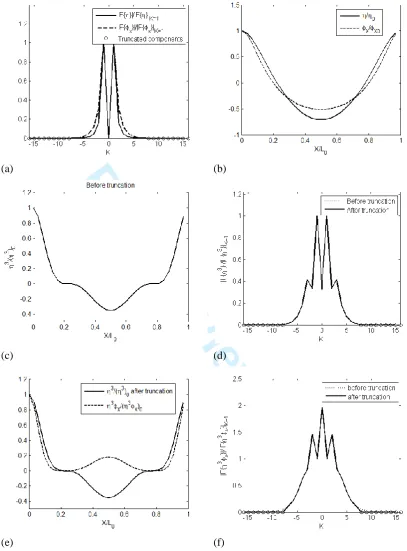
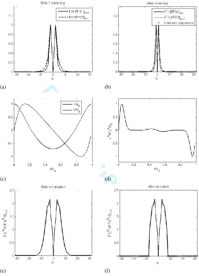
example, in order to estimate 𝐹{𝜂2𝑉}, which is a part 𝑉₄(1) and is the 3rd order

convolution, the spectrum of 𝜂 and 𝑉 will be truncated to −32/4~32/4 from the range of −32/2~32/2 as shown in Figure 10(a) for 𝑁 = 32, where the points circled out are padded as zero. Then the product of 𝜂2𝑉 is calculated in the physical spatial domain after applying inverse Fourier transform to give both 𝜂 and 𝑉, as shown in Figure 10(b) and (c). At last, the product of 𝜂2𝑉 is transformed back to

spectral space and their spectra 𝐹{𝜂2𝑉} are truncated to – 32/4~32/4, which is

illustrated in Figure 10(d). Similarly, to estimate 𝐹{𝑉𝜂6}, which is a part of 𝑉₄(3) and

is the 7th _{order convolution. The spectra of 𝜂 and 𝑉 are truncated to – 32/8~32/8}

before calculating 𝑉𝜂6, as shown in Figure 10(e). After the multiplication of the functions in physical space (Figure 10(f) and (g)), the spectrum 𝐹{𝑉𝜂6} is truncated to −32/8~32/8 (Figure 10(h)).

(a) (b)

Peer Review Only

(e) (f)

(g) (h)

Figure 10. Illustration of TAA1

TAA2: (Repeated 2/4-rule). This technique was suggested and referred as repeated 4-half rule by Clamond & Grue [1] and Fructus et al. [4]. The spectrum width of convolutions of the 2nd and 3rd order are truncated to −𝑁/4~𝑁/4. Convolutions of 4th _{order and higher will be estimated using a repeated 2/4-rule, in which the}

convolution is broken down into several terms, each one being of lower than the 3rd

order. Each individual term is estimated with 2/4-rule. For example, 𝐹{𝜂3∇𝜙̃} is

firstly split into 𝐹{𝜂3} ∗ 𝐹{∇𝜙̃}. Applying the 2/4-rule (same as in TAA1) gives 𝜂3

and ∇𝜙̃ separately (Figure 11(a) – (d) and then 𝜂3∇𝜙̃ (Figure 11(e)) in the physical

space. After that, 𝐹{𝜂3∇𝜙̃} is computed by FFT and its spectrum is truncated to

Peer Review Only

(a) (b)

(c) (d)

(e) (f)

Figure 11. Illustration of TAA2

Although this technique may work in some cases, it is found not to be accurate

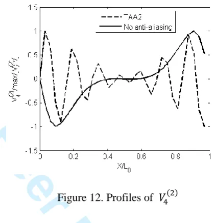
generally. For example, when the technique is applied to evaluate 𝑉₄(2) (Appendix) of

Peer Review Only

aliasing error. It can be seen that TAA2 give incorrect approximation to 𝑉₄(2) at this

resolution.

Figure 12. Profiles of 𝑉₄(2)

TAA3: (Mixed 2/4-2/8-rule). This is a new technique suggested in this paper. For this technique, the convolutions of the 2nd _{and 3}rd _{order are estimated using the 2/4-rule as}

in TAA1 and TAA2. The difference lies in dealing with the convolutions of 4th and higher order. To deal with these higher order convolutions, the spectrum of an individual function is padded as zero in the ranges of −𝑁~ − 𝑁/4 and 𝑁/4~𝑁, and then they are inversed to the physical domain. The products of the functions are found before transformed into spectral space. The resulting spectrum is truncated to

Peer Review Only

(a) (b)

(c) (d)

(e) (f)

Figure 13. Illustration of TAA3

4.2. Preliminary comparisons of different anti-aliasing techniques

In order to show which one of three anti-aliasing techniques yields better results, preliminary comparative studies have been carried out and some results are presented and discussed in this sub-section. More comparison will be given in later sections. For this purpose, the convolution parts of 𝑉3 and 𝑉4 for the Stokes waves of different

Peer Review Only

using the above three anti-aliasing techniques and their results will be compared. The aliasing error will be estimated by

𝐸𝑟𝑟𝑜𝑟{𝑉₃+ 𝑉₄} =∫ (|𝑉3,𝐶

(𝑁=2𝑛₎

− 𝑉_3,𝐶 (𝑁=29)| + |𝑉_4,𝐶 (𝑁=2𝑛)− 𝑉_4,𝐶 (𝑁=29)|) 𝑑𝑿

∫|𝑉|𝑑𝑿 (42)

where 𝑉_3,𝐶 (𝑁=2𝑛) and 𝑉_4,𝐶 (𝑁=2𝑛) are the convolution parts of 𝑉3 and 𝑉4 with

resolution of 2𝑛 ∗ 2𝑛 estimated by using one of three anti-aliasing techniques.

𝑉_3,𝐶 (𝑁=29) and 𝑉_4,𝐶 (𝑁=2 9₎

are the convolution parts of 𝑉₃ and 𝑉₄ computed by using a

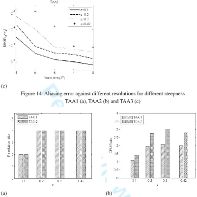
resolution of 29∗ 29, which is tested to be the resolution to eliminate the aliasing error without use of any anti-aliasing technique. The aliasing errors corresponding to three methods are plotted in Figure 14. It can be seen that the aliasing errors decrease with increase of resolution but they are larger for larger steepness. The TAA3 clearly over-performs relative to the other two techniques for stronger nonlinear waves, such as these with 𝜀 = 0.3 and 0.42. In these cases, the error of TAA3 is less than 1E-6 at the resolution of 26∗ 26 but the errors of other two is larger than 1E-6 at the resolution.

To further demonstrate the fact, Figure 15(a) presents the minimum resolution required to achieve the results with error less than 1E-6 by the three different techniques. For the same purpose, Figure 15(b) gives the ratio of CPU time corresponding to the three techniques for evaluating the convolution parts of 𝑉₃ and

𝑉4 in one time step. The ratio is estimated by dividing the CPU time of each

technique by the CPU time of TAA3. The results clearly indicate that the TAA3 is superior to the others in suppressing the aliasing errors, in particular in estimating the higher order convolutions.

Peer Review Only

(c)

Figure 14. Aliasing error against different resolutions for different steepness TAA1 (a), TAA2 (b) and TAA3 (c)

(a) (b)

Figure 15. Resolution (a) and CPU ratio (b) to achieve 𝐸𝑟𝑟𝑜𝑟{𝑉3+ 𝑉4} < 1E − 6 for

different values of steepness (Ratio = value of the method with TAA1 or TAA2 /value of the method with TAA3)

5. TECHNIQUE FOR DETERMINING THE CRITICAL VALUE 𝐷𝑐

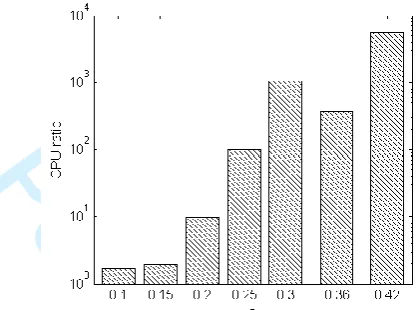
As indicated in Table I, one may use one of three schemes to evaluate the velocity 𝑉. Fructus et al. [4] used the Scheme 1 while Grue [3] employed Scheme 2 with excluding the estimation of the integral parts. Although more convolution terms need to be evaluated in Scheme 2 than Scheme 1, Scheme 2 is expected to be much more efficient as there is no need of evaluating integral parts. To demonstrate this, the ratio of CPU time taken by Scheme 1 to that of Scheme 2 is plotted in Figure 16. The results in this figure are obtained by using the two schemes to model the similar waves in Figure 6 up to a time of 1000𝑇0 in a domain of 2𝐿 ∗ 2𝐿 for different

Peer Review Only

However, it is not always true. This can be understood from the fact that Scheme 2 is derived from Scheme 1 by expanding 𝑉₃ and 𝑉₄ up to the 7th _{order (𝜀}7_{) as shown}

in Appendix. Based on this, Scheme 2 should be only accurate when the maximum gradient of the free surface is less than a critical value 𝐷_𝑐. So far, such a critical value has not been quantified, which will be discussed in the following sections.

Figure 16. Ratio of CPU time taken by Scheme 1 to that of Scheme 2 for 𝐸𝑟𝑟1< 2.5%

5.1. Estimation of magnitude of 𝐷𝑐

As has been noted in section 2.1, 𝐷 represents the local gradient of waves and thus its maximum should have a similar order to the wave steepness 𝜀 if the wave does not reach the overturning point. In order to estimate the magnitude of 𝐷_𝑐, we may assume that |𝐷|𝑚𝑎𝑥 ≈ 𝜀. In addition, the magnitude of 𝐷𝑐 must be related to the

highest order of differences between Scheme 2 and Scheme 3 or Scheme 1. From Table I, the differences come from ignoring 𝑉_3,𝐼 and 𝑉_4,𝐼. From Equation (26) and (27), the leading order of 𝑉_3,𝐼 and 𝑉_4,𝐼 are 𝑂(𝜀8) and 𝑂(𝜀9) respectively. As the former is one order higher than the latter, the magnitude of 𝐷_𝑐 may be estimated by using only 𝑉_3,𝐼. To give more specific information about the order of 𝑉_3,𝐼, it has been expanded in Appendix to

𝑉3,𝐼 = 𝑉3(3)+ 𝑂(𝜀10) (43)

where 𝑉₃(3) is given in Equation A. 8. To be more specific, let us consider a simple

wave described by 𝜂 = 𝜀𝑐𝑜𝑠𝑋 and 𝜙̃ = 𝜀𝑠𝑖𝑛𝑋, for which 𝑉 = 𝜀𝑠𝑖𝑛𝑋. For this wave, one obtains, as shown in Equation A. 9,

𝑂(𝑉3,𝐼)~𝑂(𝑉3(3))~

69

2560𝜀8sin(2𝑋) (44)

Thus

𝑂 (𝑉3,𝐼 𝑉 ) ~

69

2560𝜀7 (45)

Peer Review Only

𝑚𝑎𝑥|𝑉₃(3)|

𝑚𝑎𝑥|𝑉| (46)

It is clear that the order of 𝐸𝑟𝑟𝑜𝑟₁{𝑉} is 𝑂(𝜀7). For the simple wave, it follows that

𝐸𝑟𝑟𝑜𝑟2{𝑉}~

69 2560 𝜀8

𝜀 =

69 2560𝜀7 ≈

69

2560|𝐷|𝑚𝑎𝑥7

(47)

5.2. Values of 𝐷_𝑐 determined by numerical tests

In this subsection, tests will be carried out to further quantify the critical value 𝐷_𝑐. To do so, the error of Scheme 2 is estimated by

𝐸𝑟𝑟𝑜𝑟3{𝑉} = ∫|𝑉

(𝑠𝑐ℎ𝑒𝑚𝑒 2)_{− 𝑉}(𝑠𝑐ℎ𝑒𝑚𝑒 3)_|𝑑𝑋

∫|𝑉(𝑠𝑐ℎ𝑒𝑚𝑒 3)_{| 𝑑𝑋} (48)

where 𝑉(𝑠𝑐ℎ𝑒𝑚𝑒 3) is the profile of the velocity 𝑉 calculated by using Scheme 3 at an instant, which takes into account of all the terms, and 𝑉(𝑠𝑐ℎ𝑒𝑚𝑒 2) is the profile of velocity 𝑉 computed by Scheme 2 at the corresponding instant excluding the integral parts. The simulation is first carried out by using Scheme 3, and the data of 𝑉, 𝜙̃ and

𝜂 at all time steps are saved in files. From these data, |𝐷|𝑚𝑎𝑥 is computed for every

time step. Then Scheme 2 is employed to estimate the error in Equation (48), corresponding to the value of |𝐷|_𝑚𝑎𝑥 at each time step. Using the information, one can find the critical value Dc for a specified error. The results for three cases will be presented below.

The first case is about a Stokes wave steepened by a moving pressure on the surface. The initial wave of 𝜀 = 0.15 is obtained in the same way as for Figure 6. The domain covers one wave length (𝐿 × 𝐿) and is resolved by 27_*27 _{points. The duration}

of the simulation is 5 wave periods (𝑇₀). The pressure distribution on the free surface is specified as

𝑝(𝑋, 𝑇) = {_{0 , 𝑇 > 𝑇}−𝑝0sin(2𝜋𝑇/𝑇0) sin(𝑋 − 𝐶𝑇) , 0 ≤ 𝑇 ≤ 𝑇0/2

0/2 (49)

where 𝑝₀ = 0.25 is the amplitude of the pressure and 𝐶 = 𝐿/𝑇₀ is the wave phase speed. The wave profiles at some time steps (𝑇/𝑇₀ = 0.1, 0.4 and 0.88) obtained by Scheme 3 are shown in Figure 17(a). It demonstrates that the free surface elevation gradually becomes steeper and steeper. The errors in Equations (46), (47) and (48) corresponding to the values of |𝐷|_𝑚𝑎𝑥 are presented in Figure 17(b). It shows that the errors estimated for Scheme 2 using Equations (46) and (48) is less than 2E-4 and does not increases significantly when |𝐷|_𝑚𝑎𝑥 ≤ 0.5, while it grows exponentially when |𝐷|_𝑚𝑎𝑥 exceeds 0.5. In addition, the errors of Scheme 2 have the same trend as

the expression of ₂₅₆₀69 |𝐷|_𝑚𝑎𝑥7 in Equation (47). Furthermore, the errors estimated by

using Equation (46) are closely correlated with these of Equation (48).

Peer Review Only

(a) (b)

Figure 17. Wave profiles at different instants (a) and numerical error against maximum

gradient (b) for 𝑝0 = 0.25

(a) 𝑝₀= 0.22 (b) 𝑝₀ = 0.3

Figure 18. Numerical error against maximum gradient for different pressure amplitude

The second case tested is related to a 2D Benjamin-Feir instability [11]. To do this test, the wave with 𝜀 = 0.22 generated as in Figure 6 is disturbed by

𝛿𝜂 = 0.105𝜀𝑐𝑜𝑠 (9 8𝑋 −

𝜋

4) + 0.105𝜀𝑐𝑜𝑠 ( 7 8𝑋 −

𝜋

4) (50)

Peer Review Only

(a) (b)

Figure 19. Wave profiles at different instants (a) and numerical error against maximum gradient (b)

The third case considered is about a wave of 𝜀 = 0.2985 generated as in Figure 6 but perturbed by a directional side-band waves

𝛿𝜂 =0.05𝜀

2 [𝑠𝑖𝑛(𝑲𝟏∙ 𝑿) + 𝑠𝑖𝑛(𝑲𝟐∙ 𝑿)] (51)

where 𝑲_𝟏= (3/2, 4/3) and 𝑲_𝟐= (3/2, −4/3). The computational domain covers

2𝐿 × 1.5𝐿 on transversal and longitudinal direction and is resolved by 28_*28 _points.

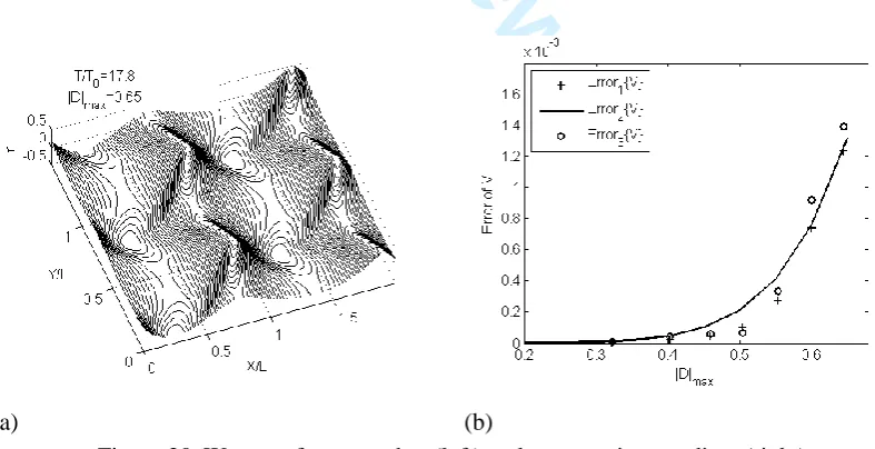
The duration of the simulation is 18 wave periods. During the simulation, the waves grow into horse-shoe pattern eventually at 𝑇/𝑇₀ = 17.8, as shown in Figure 20(a). The error of Scheme 2 is shown on the right in Figure 20(b). This again indicates that the error is insignificant when |𝐷|_𝑚𝑎𝑥 ≤ 0.5.

(a) (b)

Figure 20. Wave surface snapshot (left) and error against gradient (right)

All the above cases for different kinds of wave evidence that one may take 0.5 as the critical value (𝐷_𝑐) if the error of 2E-4 is acceptable, under which Scheme 2 may be applied with ignoring the integral parts in the velocity 𝑉. They evidence also that

Peer Review Only

Equation (46) is more general than Equation (47) as the former is not based on specific waves. In practice, one may take 𝐷_𝑐 = 0.5 or use Equation (46) to determine

𝐷𝑐 for a specified error. More generally, one may numerically estimate the error by

using Equation (46). If using this way, the condition of |𝐷|_𝑚𝑎𝑥 ≤ 𝐷_𝑐 in Figure 2 must be replaced by 𝐸𝑟𝑟𝑜𝑟₁{𝑉} ≤ 𝐸𝑟𝑟𝑜𝑟_𝑐, where 𝐸𝑟𝑟𝑜𝑟_𝑐 is the tolerant error.

6. OVERALL EFFICIENCY OF THE IMPROVED METHOD

Up to now, three new techniques have been discussed. They are developed in order to accelerate the computation of the Spectral Boundary Integral Method originally proposed in [1-4]. In this section, the overall efficiency of the improved method equipped with the de-singularity technique for weakly singular integrals, the anti-aliasing technique and the mixed scheme (Figure 2) will be discussed. For this purpose, the convergent properties and CPU time of the method in [4] and the improved method of this paper will be compared. Both methods are employed to simulate the waves similar to that in Figure 20 but with different initial steepness, i.e,

𝜀 = 0.1, 0.2 and 0.3, respectively. For each of the cases, different resolutions are used, which are 25*25, 26*26, 27*27 and 28*28. The simulation is carried out until

𝑇/𝑇₀ = 18.

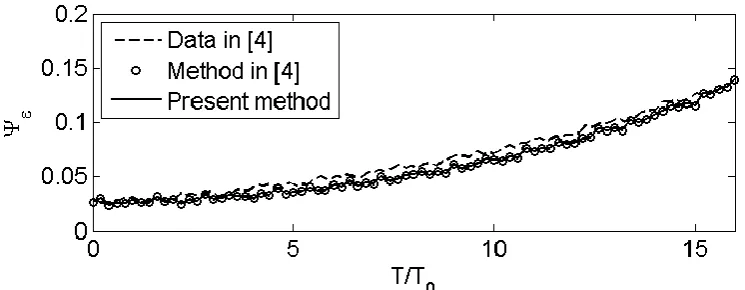
For this case, Fructus et al. [4] presented a quantitative result of the following ratio for 𝜀 = 0.2985

Ψ_𝜖 =|𝐹{𝜂}|(𝑲=(3/2,4/3),𝑇)

|𝐹{𝜂}|_{(𝑲=(1,0),𝑇=0)} (52)

where |𝐹{𝜂}|_{(𝑲=(3/2,4/3),𝑇)} is the value of the spectrum at a time T corresponding to

Peer Review Only

Figure 21. Evolution of perturbation components of 𝑲 = (3/2, 4/3)

The free surface profiles at three sections (𝑌 = 3𝐿0/4, 𝑋 = 𝐿0 and 𝑋 = 4𝑌/3)

obtained by the code based on the Method in [4] and our improved method are shown in Figure 22. There is no visible difference between them. Their quantitative difference is of ∫(|𝜂₁− 𝜂₂|)𝑑𝑿 / ∫|𝜂₂|𝑑𝑿 ≈ 0.2%, where 𝜂₁ is the free surface elevation at 𝑇/𝑇₀ = 18 obtained from the method in [4] and 𝜂₂ is that from the improved method, both for resolution of 28*28. This demonstrates that both the methods will produce almost the same results when the resolution is sufficiently high.

(a)

Peer Review Only

(c)

Figure 22. Free surface profiles at different section for 𝜀 = 0.3

However, their convergent rate may be different. To examine this, we define the error of the wave elevation as

𝐸𝑟𝑟𝑜𝑟₂{𝜂} = ∫(|𝜂(𝑁=2

𝑛₎

− 𝜂_𝐵|)𝑑𝑿 ∫|𝜂𝐵|𝑑𝑿

(53)

where 𝜂(𝑁=2𝑛) is the solution obtained by using a method with resolution 2𝑛∗ 2𝑛 at

𝑇/𝑇0 = 18 and 𝜂𝐵 is the solution with sufficiently high resolution. Here 𝜂𝐵 is

selected as that for Figure 22. The errors of two methods corresponding to different initial steepness are plotted in

Peer Review Only

(c)

Figure 233, together with the lines representing (∆𝑋)𝑠 where ∆𝑋 denotes the element size. It shows that the convergent rate of the improved method is closed to the 4th _{order for all the cases.}

In addition, the CPU time used by the two methods to achieve the results with error less than 0.2% is also investigated. Figure 24 depicts the ratio of the CPU time used by the Method in [4] to that of the improved method. It indicates that for waves with moderate steepness (𝜀 ≤ 0.1), the CPU time of both the methods is similar. When the steepness increases, the advantage of the improve method over the Method in [4] is obvious. For instance, in the case of 𝜀 = 0.2985≈ 0.3, the ratio is more than 35. Of course, if the requirement on the accuracy is not so high, the CPU time ratio may not be thus large. We do examine the wave profiles with different errors. The profiles along the transversal direction corresponding to different error values are shown in Figure 25. It can be seen that the profile with an error of about 0.6% calculated by Equation (54) would be quite different. The error of about 0.2% is needed to achieve invisible result based on our observation.

Peer Review Only

(c)

Figure 23. Convergent rate of different methods for 𝜀 = 0.1, 0.2 and 0.3

Figure 24. CPU ratio against steepness at error less than 0.2%

Figure 25. Profiles corresponding to different errors

7. CONCLUSION

Peer Review Only

gradient for the mixed scheme illustrated in Figure 2. It has demonstrated that the improved method equipped with the techniques can significantly accelerate the computation, in particular in the cases with strong nonlinearity. In some cases, it has been observed to be more than 35 time faster than the method without the techniques.

APPENDIX

Equation (19) is re-written as

𝐹{𝑉3}=_{2𝜋 𝐹}𝐾 {∫ 𝜙̃′[1 −(1 + 𝐷2) −3/2

]∇′∙[(𝜂′− 𝜂)∇′_𝑅1]𝑑𝑿′

𝑆0

} A. 1

The term involving in the local gradient is expanded in the Taylor series

1 − (1 + 𝐷2₎−3/2 ₌3

2𝐷2− 15

8 𝐷4+ 35

16𝐷6… A. 2

Using it, 𝑉3 becomes

𝐹{𝑉3}=_{2𝜋 𝐹}𝐾 {3₂∫𝜙̃′𝐷2∇′∙[(𝜂′− 𝜂)∇′1_𝑅]𝑑𝑿′

−15₈ ∫𝜙̃′𝐷4∇′∙[(𝜂′− 𝜂)∇′_𝑅1]𝑑𝑿′

+∫𝜙̃′[1 −(1 + 𝐷2)−3/2−3_{2 𝐷}2+15_{8 𝐷}4]∇′

∙[(𝜂′− 𝜂)∇′_𝑅1]𝑑𝑿′}

=𝐹{𝑉₃(1)}+ 𝐹{𝑉₃(2)}+ 𝐹{𝑉_3,𝐼}

A. 3

where

𝐹 {𝑉₃(1)} = −𝐾₆[𝐾𝑖𝑲 ∙ 𝐹{𝜂3∇𝜙̃ }− 3𝐹{𝜂𝐹−1{𝐾𝑖𝑲 ∙ 𝐹{𝜂2∇𝜙̃ }}}

+ 3𝐹{𝜂2𝐹−1{𝐾𝑖𝑲 ∙ 𝐹{𝜂∇𝜙̃ }}}+ 𝐹{𝜂3𝐹−1{𝐾3𝐹{𝜙̃ }}}]

A. 4

and

𝐹 {𝑉₃(2)}= −₁₂₀𝐾 [𝑖𝑲𝐾3∙ 𝐹{𝜂5∇𝜙̃ }− 5𝐹{𝜂𝐹−1{𝑖𝑲𝐾3∙ 𝐹{𝜂4∇𝜙̃ }}}

+ 10𝐹{𝜂2𝐹−1{𝑖𝑲𝐾3∙ 𝐹{𝜂3∇𝜙̃ }}}

− 10𝐹{𝜂3𝐹−1{𝑖𝑲𝐾3∙ 𝐹{𝜂2∇𝜙̃ }}}

+ 5𝐹{𝜂4𝐹−1{𝑖𝑲𝐾3∙ 𝐹{𝜂∇𝜙̃ }}}

+ 𝐹{𝜂5𝐹−1{𝐾5𝐹{𝜙̃ }}}]

A. 5

Peer Review Only

terms in 𝑉₃(1) and 𝑉₃(2) , respectively. Therefore the equations above need less

calculation.

In order to estimate the leading order of 𝑉_3,𝐼, the expansion goes further to the 8th

order convolution

𝐹{𝑉3,𝐼} =_{2𝜋 𝐹}𝐾 {35₁₆∫𝜙̃′∇′∙[(𝜂′− 𝜂)∇′_𝑅1]𝐷6𝑑𝑿′

+∫𝜙̃′[1 −(1 + 𝐷2)−3/2−3_{2 𝐷}2+15_{8 𝐷}4−35_{16 𝐷}6]∇′

∙[(𝜂′− 𝜂)∇′1_𝑅]𝑑𝑿′}

= 𝐹 {𝑉₃(3)} +_{2𝜋 𝐹}𝐾 {∫𝜙̃′[1 −(1 + 𝐷2)−3/2−3_{2 𝐷}2+15_{8 𝐷}4−35_{16 𝐷}6]∇′

∙[(𝜂′− 𝜂)∇′_𝑅1]𝑑𝑿′}

A. 6

where

𝐹 {𝑉₃(3)} =_{2𝜋 𝐹}𝐾 {35₁₆∫𝜙̃′∇′∙[(𝜂′− 𝜂)∇′1_𝑅]𝐷6𝑑𝑿′}

= −₅₀₄₀𝐾 [𝑖𝑲𝐾5∙ 𝐹{𝜂7∇𝜙̃ }− 7𝐹{𝜂𝐹−1{𝑖𝑲𝐾5∙ 𝐹{𝜂6∇𝜙̃ }}}

+ 21𝐹{𝜂2𝐹−1{𝑖𝑲𝐾5∙ 𝐹{𝜂5∇𝜙̃ }}}

− 35𝐹{𝜂3𝐹−1{𝑖𝑲𝐾5∙ 𝐹{𝜂4∇𝜙̃ }}}

+ 35𝐹{𝜂4𝐹−1{𝑖𝑲𝐾5∙ 𝐹{𝜂3∇𝜙̃ }}}

− 21𝐹{𝜂5𝐹−1{𝑖𝑲𝐾5∙ 𝐹{𝜂2∇𝜙̃ }}}

+ 7𝐹{𝜂6𝐹−1{𝑖𝑲𝐾5∙ 𝐹{𝜂∇𝜙̃ }}}+ 𝐹{𝜂7𝐹−1{𝐾7𝐹{𝜙̃ }}}]

A. 7

Therefore

𝑉₃(3) = − 1

5040𝐹−1{𝑖𝑲𝐾6∙ 𝐹{𝜂7∇𝜙̃} − 7𝐾𝐹 {𝜂𝐹−1{𝑖𝑲𝐾5∙ 𝐹{𝜂6∇𝜙̃}}}

+ 21𝐾𝐹 {𝜂2_𝐹−1_{{𝑖𝑲𝐾}5_{∙ 𝐹{𝜂}5_∇𝜙̃}}}

− 35𝐾𝐹 {𝜂3_𝐹−1_{{𝑖𝑲𝐾}5_{∙ 𝐹{𝜂}4_∇𝜙̃}}}

+ 35𝐾𝐹 {𝜂4_𝐹−1_{{𝑖𝑲𝐾}5_{∙ 𝐹{𝜂}3_∇𝜙̃}}}

− 21𝐾𝐹 {𝜂5_𝐹−1_{{𝑖𝑲𝐾}5_{∙ 𝐹{𝜂}2_∇𝜙̃}}}

+ 7𝐾𝐹 {𝜂6_𝐹−1_{{𝑖𝑲𝐾}5 _{∙ 𝐹{𝜂∇𝜙̃}}} + 𝐾𝐹 {𝜂}7_𝐹−1_{𝐾7_{𝐹{𝜙̃}}}}}

Peer Review Only

For 𝜂 = 𝜀𝑐𝑜𝑠𝑋, 𝜙̃ = 𝜀𝑠𝑖𝑛𝑋 and 𝑉 = 𝜀𝑠𝑖𝑛𝑋, one obtains that

𝑉₃(3)= − 1 5040

𝜀8

128[−17388 sin(2𝑋)+ 3024 sin(4𝑋)− 12 sin(6𝑋)]

~₂₅₆₀69 𝜀8_sin(2𝑋)

A. 9

Similarly, the local gradient term of 𝑉4 in Equation (20),

𝑉4 = 𝐹−1{

𝐾 2𝜋𝐹 {∫

𝑉′

𝑅 (1 − 1

√1 + 𝐷2) 𝑑𝑿 ′ 𝑆0

}} A. 10

can also be expanded in the Taylor series

1 − 1 √1 + 𝐷2 =

1 2𝐷2−

3 8𝐷4+

5

16𝐷6+ ⋯ A. 11

Then this integration of 𝑉4 could be rewritten as

𝐹{𝑉₄} = 𝐾 2𝜋𝐹 {∫

𝑉′

𝑅 1

2𝐷2𝑑𝑿′− ∫ 𝑉′

𝑅 3

8𝐷4𝑑𝑿′+ ∫ 𝑉′

𝑅 5

16𝐷6𝑑𝑿′ + ∫𝑉

′

𝑅 (1 − 1 √1 + 𝐷2 −

1 2𝐷2+

3 8𝐷4 −

5

16𝐷6) 𝑑𝑿′} = 𝐹{𝑉₄(1)} + 𝐹{𝑉₄(2)} + 𝐹{𝑉₄(3)} + 𝐹{𝑉_4,𝐼}

A. 12

where

𝐹{𝑉₄(1)} = −𝐾

2[𝐾𝐹{𝜂2𝑉} − 2𝐹 {𝜂𝐹−1{𝐾𝐹{𝜂𝑉}}} + 𝐹 {𝜂2_𝐹−1_{{𝐾𝐹{𝑉}}}]}

A. 13

𝐹{𝑉₄(2)} = − 𝐾

24[𝐾3𝐹{𝑉𝜂4} − 4𝐹 {𝜂𝐹−1{𝐾3𝐹{𝑉𝜂3}}} + 6𝐹 {𝜂2_𝐹−1_{𝐾3_{𝐹{𝑉𝜂}2_}}}

− 4𝐹 {𝜂3_𝐹−1_{𝐾3_{𝐹{𝑉𝜂}}} + 𝐹 {𝜂}4_𝐹−1_{𝐾3_{𝐹{𝑉}}}]}

A. 14

𝐹{𝑉₄(3)} = −𝐾

720[𝐾5𝐹{𝑉𝜂6} − 6𝐹 {𝜂𝐹−1{𝐾5𝐹{𝑉𝜂5}}} + 15𝐹 {𝜂2_𝐹−1_{𝐾5_{𝐹{𝑉𝜂}4_}}}

− 20𝐹 {𝜂3_𝐹−1_{𝐾5_{𝐹{𝑉𝜂}3_}}}

+ 15𝐹 {𝜂4_𝐹−1_{𝐾5_{𝐹{𝑉𝜂}2_}}}

− 6𝐹 {𝜂5_𝐹−1_{𝐾5_{𝐹{𝑉𝜂}}} + 𝐹 {𝜂}6_𝐹−1_{𝐾5_{𝐹{𝑉}}}]}

A. 15