Numerical Investigation of breaking waves and their interations with structures using MLPG_R method

      

City, University of London Institutional Repository

Citation

:

Zhou, J. (2010). Numerical Investigation of breaking waves and their interations with structures using MLPG_R method. (Unpublished Doctoral thesis, City University

London)

This is the accepted version of the paper.

This version of the publication may differ from the final published

version.

Permanent repository link: http://openaccess.city.ac.uk/8729/

Link to published version

:

Copyright and reuse:

City Research Online aims to make research

outputs of City, University of London available to a wider audience.

Copyright and Moral Rights remain with the author(s) and/or copyright

holders. URLs from City Research Online may be freely distributed and

linked to.

City Research Online: http://openaccess.city.ac.uk/ [email protected]

Zhou, Juntao (2010). Numerical investigation of breaking waves and their interactions with structures using MLPG_R method. (Unpublished Doctoral thesis, City University London)

City Research Online

Original citation: Zhou, Juntao (2010). Numerical investigation of breaking waves and their interactions with structures using MLPG_R method. (Unpublished Doctoral thesis, City University London)

Permanent City Research Online URL: http://openaccess.city.ac.uk/1083/

Copyright & reuse

City University London has developed City Research Online so that its users may access the research outputs of City University London's staff. Copyright © and Moral Rights for this paper are retained by the individual author(s) and/ or other copyright holders. All material in City Research Online is checked for eligibility for copyright before being made available in the live archive. URLs from City Research Online may be freely distributed and linked to from other web pages.

Versions of research

The version in City Research Online may differ from the final published version. Users are advised to check the Permanent City Research Online URL above for the status of the paper.

Enquiries

1

NUMERICAL INVESTIGATATION OF BREAKING WAVES AND

THEIR INTERATIONS WITH STRUCTURES USING MLPG_R

METHOD

By

Juntao Zhou

Supervisor

Prof. Qingwei Ma

A thesis submitted in fulfillment of

requirement of degree of

Doctor of Philosophy

School of Engineering and Mathematical Sciences

City University, London

2

CONTENTS

LIST OF FIGURES

... 5

LIST OF TABLES

... 10

ACKNOWLEDGEMENTS

... 11

DECLARATION

... 12

ABSTRACT

... 13

LIST OF SYMBOLS

... 15

1. INTRODUCTION

... 17

1.1 Background ... 17

1.2 Objectives of the study ... 20

1.3 Outline of the thesis ... 20

2. LITERATURE REVIEW

... 22

2.1 Mesh-based methods ... 22

2.2 Meshless methods ... 23

2.2.1 Smooth Particle Hydrodynamic method (SPH) ... 25

2.2.2 Moving Particle Semi-implicit method (MPS) ... 27

2.2.3 Meshless Local Petro-Galerkin method (MLPG) ... 29

2.3 Numerical methods for calculation pressure gradient in meshless methods ... 31

2.4 Numerical methods for implementation of solid boundary condition in meshless methods ... 33

2.5 Numerical methods for identifying the free surface ... 35

3. MATHEMATICAL MODEL AND NUMERICAL METHOD

... 38

3.1 Governing equations and boundary conditions ... 38

3.2 Numerical Procedure ... 39

3.3 MLPG_R Formulation for 2D cases ... 41

3.3.1 Discretization of the governing equation for pressure ... 44

3

3.3.3 Numerical implementation of solid boundary condition ... 49

3.3.4 Test the effectiveness of parameter in Eq. (3.2.3) ... 53

3.4 MLPG_R Formulation for 3D cases ... 57

3.4.1 Numerical technique for evaluating domain integrals ... 59

3.4.2 Numerical technique for evaluating surface integrals ... 63

3.4.3 Effectiveness of the semi-analytical technique for surface integrals ... 67

4 NUMERICAL TECHUNIQUES FOR IDENTIFYING PARTICLES ON FREE SURFACE

... 71

4.1 Introduction ... 71

4.2 Mixed Particle Number Density and Auxiliary Function Method (MPAM) for 2D cases ... 72

4.3 Effectiveness of MPAM for identifying the free surface particles ... 75

4.4 Mixed Particle Number Density and Auxiliary Function Method (MPAM) for 3D cases ... 77

5. NUMERICAL SIMULATION OF DAM BREAKING

... 80

5.1 Two dimensional dam breaking ... 80

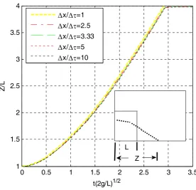
5.1.1 Convergent investigation on different values of x/ ... 84

5.1.2 Convergent investigation on different space increments x ... 86

5.2 Three-dimensional dam breaking ... 88

6. BREAKING WAVES OVER NON-FLAT SEABED

... 100

6.1 2D breaking waves on a slope ... 101

6.1.1 Convergence investigation on different value of x 



... 102

6.1.2 Convergence investigation based on different value of x ... 103

6.2 2D breaking waves over a submerged step ... 109

6.3 3D breaking waves on a slope ... 112

6.3.1 Convergence investigation on different values of x/ ... 113

6.3.2 Convergence investigation on different values of x ... 115

7. SIMULATION OF VIOLENT SLOSHING WAVES

... 118

4

7.2 Numerical investigations on 2D sloshing waves ... 121

7.2.1 Convergence investigation and numerical validation ... 121

7.2.2 Behaviors of impact pressure in a baffled tank ... 128

7.3 Numerical investigations for 3D sloshing waves ... 133

8. 3D NUMERICAL INVESTIGATIONS ON VIOLENT WAVE IMPACT ON THE CYLINDER: OFFSHORE ENERGY STRUCTURE

... 139

8.1 Investigations of relationship between pressure impact peak and breaking waves . 141 8.2 Effects of Locations of Structures ... 143

8.3 Effects of different wave heights ... 145

9. CONCLUSIONS AND FUTURE WORK

... 147

9.1 Numerical techniques ... 148

9.2 Two dimensional and three dimensional sloshing cases ... 149

9.3 Interaction between breaking waves and a fixed cylinder ... 149

9.4 Future work ... 150

REFERENCES

... 151

APPENDIX A: PUBLICATION LIST

... 162

5

LIST OF FIGURES

Fig.1.1.1 Wave breaking in sea……….………..……….……….17 Fig.1.1.2 Breaking wave impacting on a ship……….………..17 Fig.2.4.1 Illustration of the influence domain for wall particles in (a) BC1, (b) BC2 and (c)

BC3 (solid circle: wall particles; hollow circle: water particles)…………..……....32 Fig.3.0.1 Schematic of computational domain and the coordinate ….……..………….……..38 Fig.3.3.1 Illustration of particles, integration domain and support domain (a: wall particle; b: free surface particles and c: inner particles)……….….…40 Fig.3.3.2 Illustration of division of an integration domain………...……….…...44 Fig.3.3.3 Illustration of the influence domain for wall particles (solid circle: wall particles;

hollow circle: water particles)………..….49 Fig.3.3.4 Schematic of different solid boundaries……….………..….50 Fig.3.3.5 Schematic analysis of normal derivative for d boundary particle…….…….…..….52 Fig.3.3.6 Effects of different  on the PND in dam breaking cases …....………….……....55 Fig.3.3.7 Configurations of particles for the cases with different value of ……….………57 Fig.3.4.1.Illustration of division of an integration domain………..……….59 Fig.3.4.2 Illustration of integration domain in -plane……….………..………64 Fig.3.4.3 A schematic view of the tank……….………67 Fig.3.4.4 Comparison of static pressure obtained by using the Gaussian quadrature and the

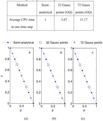
semi-analytical technique for estimating the surface integral………..68 Fig.3.4.5 Comparison of wave profiles at different instants obtained by using the

semi-analytical technique and the Gaussian quadrature with 32 and 72 Gaussian points, respectively………..…………..………...70 Fig.4.2.1 Two typical examples of incorrect identification of free surface particles. (Solid

6

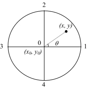
represents inner particle identified by the PNDM)………..……….74 Fig. 4.2.2 Local coordinate system at Particle I (inner circle denotes integration domain of the

particle; outer circle denotes the support domain on it)……….………..…74 Fig.4.3.1 Comparisons of particle configurations obtained by using different free surface

identification techniques (black color: free surface particles; grey or blue color: wall particles or inner particles)……….…………..…76 Fig.4.3.2 Snapshots of the water particles in pre-breaking stage (Blue particles: inner water

particle; Black particles: free surface particle; Grey particles: sloping seabed and Red line: experiment data (Li & Raichlen, 1998))………..….77 Fig.4.3.3 Snapshots of the water particles in the post-breaking stage (Blue particles: inner

water particle; Black particles: free surface particle; Grey particles: sloping seabed)………..…………78 Fig.4.4.1 Local domain at Node I for the definition of auxiliary function (the inner sphere

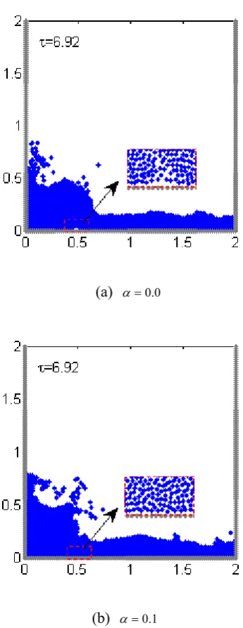
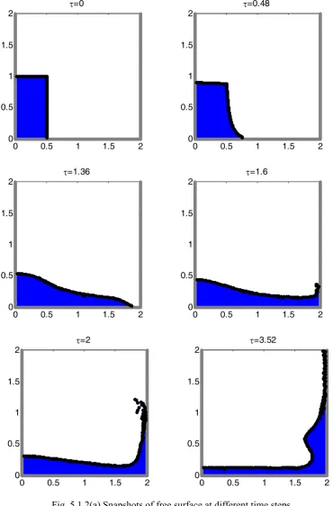
denotes integration domain of the particle; the outer sphere denotes the support domain; the 6 coloured cylinders have the same diameter as the inner sphere)……….79 Fig.5.1.1 Dam breaking: problem definition.………...80 Fig.5.1.2(a) Snapshots of free surface at different time steps (grey particles: wall; the black

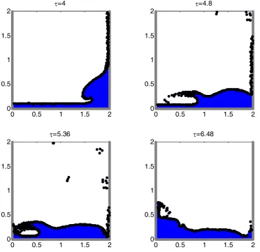
ones: free surface particles) ………..……….81 Fig.5.1.2(b) Snapshots of free surface at different time steps (grey particles: wall; the black

ones: free surface particles)………….………..82 Fig.5.1.3 Comparing the motion of the leading edge with other simulated results and

experiment data………..83 Fig.5.1.4 Comparing the motion of the leading edge corresponding different values

ofx/ ………..………..84 Fig.5.1.5 Non-physical occurrence with x/ =1……….….85 Fig.5.1.6 Comparing free surface profiles corresponding to different values ofx/ .…..86 Fig.5.1.7 Comparing free surface profiles corresponding to different values ofx with

5 . 2 / 

7

Fig.5.2.1 Schematic view of the tank and the obstacle (unit: m)……….………....89 Fig.5.2.2 Details of the obstacle and the pressure transducers (unit: m)……….……...89 Fig.5.2.3 General description of the system: top (top picture) and side (bottom picture) views Fig.5.2.4 Snapshots of the free surface at (a) t=0.227s (b) t=0.493s and (c) t=0.701s……...90 Fig.5.2.5 Comparison of the free surface profiles at t 0.4s (a: experiment, b: FVM

numerical results, both results from Klessfsman, et al, 2005; c: present method)………...91 Fig.5.2.6 Comparison of the free surface profiles at t 0.56s (a: experiment, b: FVM

numerical results, both results from Klessfsman, et al, 2005; c: present method)………...92 Fig.5.2.7 The time histories of free surface elevations at (a) for H2, (b) for H3 and (c) for

H4………93 Fig.5.2.8 Pressure time histories at (a) for P1, (b) for P2 and (c) for P3…….…………....….94 Fig.5.2.9 Pressure time histories at (a) for P5, (b) for P6, (c) for P7 and (d) for P8….……...96 Fig.5.2.10 Comparison of free surface profile at the same time (a) results without smoothing,

(b) results with smoothing……..………..………..…98 Fig.5.2.11 Pressure time histories at (a) for P5, (b) for P6, (c) for P7 and (d) for P8………..99 Fig.6.0.1 Illustration of model set-up for the solitary wave….……...………..………..100 Fig.6.1.1 Comparison between experimental wave profiles (Li and Raichlen, 1998) and

numerical results for different values of x ………...104

Fig.6.1.2 Comparison between experimental wave profiles [Li and Raichlen (1998)] and numerical results obtained by using different x values when

5  

x  …..………..105

Fig.6.1.3 Wave profiles in the post-breaking stage obtained by using different values of x

at when x 5………..…...106 Fig.6.1.4 Comparisons between laboratory photographs (Li and Raichlen, 2003) and

8

Fig.6.2.2 Snapshots of solitary wave evolution over the step at different time steps…….…100 Fig.6.2.3 Comparisons of wave elevations between the numerical results (line) and

experimental data (mark) (Yasuda et al, 1997) at three different gauges (P1, P2 and P3)...………..………111 Fig.6.2.4 Velocity field around the step when wave crest is passing by……….112 Fig.6.3.1 Comparison between experimental wave profiles (Li and Raichlen, 1998) and

numerical results for different values of x ………..……….114

Fig.6.3.2 Comparisons between experimental wave profiles [Li and Raichlen (1998)] and numerical results obtained by using different xwhen x/ 5……..…….116 Fig.6.3.3 Wave profiles in the post-breaking stage obtained by using different values of

x

 when x/ 5………..………...117 Fig.7.2.1 Schematic view of experimental set-up and corresponding tank sizes………...…121 Fig. 7.2.2 Comparison between the experiment and numerical results………..123 Fig.7.2.3 Time histories of pressure with different values of x/ for Nz=30………...…124 Fig.7.2.4 Time histories of pressure with different Nz for x/ =2……….….…124 Fig.7.2.5 Pressure in one period with different Nz for x/ =2………...….125 Fig.7.2.6 Wave profile corresponding to the first peak shown in Fig. 7.2.5………..…126 Fig.7.2.7 Wave profile corresponding to the first trough value shown in Fig. 7.2.5……..…126 Fig.7.2.8 Wave profile corresponding to the second peak shown in Fig. 7.2.5………….….126 Fig.7.2.9 Wave profile corresponding to the second trough shown in Fig. 7.2.5……….…..127 Fig.7.2.10 Wave profile corresponding to the third peak shown in Fig. 7.2.5………….…..127 Fig.7.2.11 Sketch of baffle and the neighbouring water particles (black solid circles: baffle

particles and wall particles; hollow circles: water particles; dash circles represent the initial influence domain; the solid curve represent effective influence domain)………..………..….129 Fig.7.2.12 Schematic view of tank and corresponding tank sizes (A: No baffle; B: Middle

9

Fig. 7.2.12 for Case A, (b) for Case B and (c) for Case C……….132 Fig.7.2.15 Comparison of pressure time histories at the point b……….…...133 Fig.7.3.1 Schematic view and sizes of the tank………...134 Fig.7.3.2 Snapshots of violent slosh wave (black particles: free surface particle; blue: velocity

field)………..………..136 Fig.7.3.3 Comparisons of the time histories of impact pressure on different record

points……….………137 Fig.8.0.1 The schematic view and details of tank and the structure………..………….……140 Fig.8.1.1 Different stages of wave impacting on the wind turbine structure (solitary wave

height is 0.7, cylinder location is C)……….………141 Fig.8.1.2 Time histories of pressure acting on the wind energy structure (solitary wave height

is 0.7, location: C; Point 1: 0.1 above the MWL; Point 2: 0.3 above the MWL)………..……….………142 Fig.8.1.3 Enlargement of free-surface particle distribution near structure viewed by x-z

coordinates (solitary wave height is 0.7, location: C,  ≈ 13.44)…………...….142 Fig.8.2.1 Free surface profiles near the structures at 13.2, which are in different locations

(solitary wave height is 0.7, a for Location A, b for Location B and c for Location C)……….……….………144 Fig.8.2.2 Pressure time histories at Point 2 on the structures located at different positions

(Point 2: 0.3 above the MWL)………..144 Fig.8.2.3 Free surface profile near the structure at  12.48at location B………...………145 Fig.8.3.1 Pressure time histories at Point 2 corresponding to different solitary wave heights

10

LIST OF TABLES

Table 3.4.1 Comparison of CPU time required by using different methods to evaluate the surface integral (GQ: Gaussian quadrature) for a static case…………..……….67 Table 3.4.2 Comparison of CPU time required by using different method to evaluate the

11

ACKNOWLEDGEMENTS

This study is sponsored by two projects, the first one is ‘

Interaction between Breaking

Waves and Three-dimensional Surface-Piercing Structures

‘funded by the Leverhulme Trust, UK and the second one is ‘Numerical investigation on violent sloshing loads in a FPSO tank’ funded by the ABS, USA , for which the author is most grateful.

I would like to express my sincere gratitude to my supervisor Dr. Q.W. Ma, for the guidance, support, assistance, friendship and understanding he has shown in helping me complete this work. His excellence in academics and personality will inspire me for my future. I would also like to thank him for his comments on the draft of this thesis.

A special thanks to Dr. Shiqiang Yan in our research group, who read the manuscript in detail. The valuable suggestions and discussions lead to a significant improvement of this thesis. I would also offer my thanks to my colleagues in the school, for their suggestions and discussion on my work.

12

DECLARATION

No portion of the work referred to in the thesis has been submitted in support of an application for other degree or qualification of this or any other university or other institute of learning.

13

ABSTRACT

Meshless Local Petrov-Galerkin method based on Rankine source solution (MLPG_R) has

been developed by Dr. Qingwei Ma (Ma, 2005b) and has been used to simulate the nonlinear water wave problems in 2D cases without the occurrence of the breaking waves. In this thesis, MLPG_R method has been further developed to numerically simulate breaking waves and the interactions between breaking waves and structures in 2D and 3D cases. The main difference between this meshless method and conventional mesh-based methods is that the governing equations are solved in terms of particle interaction models, without the need of computational meshes. Therefore, this method avoids the time-consuming mesh generating and updating procedures which may be necessary and may need to be frequently performed in the mesh-based methods. Furthermore, in order to simulate the breaking waves well, several novel numerical techniques are developed and adopted. The numerical technique for implementing the solid boundary condition for meshless methods is proposed, which is more robust than others in terms of accuracy and efficiency. A technique for meshless interpolation (SFDI scheme) is adopted, which is as accurate as the more costly moving least square (MLS) method generally but requires much less computational time than the latter. A newly developed technique for identifying the free surface particles is presented, which is much more robust than those existing in literature. A semi-analytical method for numerical evaluation of integrals in a local domain and on its surface is presented to form the matrix for the algebraic equations, which makes it possible to modelling the 3D problems on personal computers.

14

15

LIST OF SYMBOLS

d water depth

g gravitational acceleration

h wave height of solitary wave

p pressure



_,

n normal and tangential vectors, respectively

r distance between two partilces

0

r cut-off radius

mI mass of particle I

nI particle number density of particle I n0 _{initial particle number density}

*

I

n particle number density of particle I at the intermediate step



,

t dimensional time and nondimensionlised time, respectively

u velocity vector of the flow

*

u velocity vector of the flow at the intermediate time step

w

v

u

,

,

x-,y- and z-directional velocity components of fluids, respectively

x,y,z spatial coordinates in a Cartesian coordinate system, respectively

x spatial coordinate

B width of tank

Ds degree of the spatial dimensions

[K] coefficient matrix of the pressure equations [F] coefficient matrix of the pressure equations

N total number of particles in the support domain of targeted particle

Nz particle number along z-direction

16

 gradient operator

2



Laplace equation operator

t





Partial time derivative in the Cartesian coordinate system

Dt

D

substantial derivative defined as

















t

Dt

D

 kinematic viscosity



density of the fluid

I



integration domain of particle I

I



 surface domain of integration domain of particle I



test function

Dt

D

substantial derivative defined as

















t

Dt

D

U velocity of the rigid boundary

U acceleration of rigid boundary

t

 time step



shape function

W weight function

 base function



17

1. INTRODUCTION

1.1 Background

Wave breaking (see, Fig.1.1.1) is a general phenomenon in nature. This phenomenon plays a vital role in air–sea interactions and wave-structure interactions. In addition, breaking waves may release huge amounts of energy, which may severely damage coastal structures, vehicles in the sea (see, Fig.1.1.2) and threaten the lives on them. Therefore, breaking waves and their interactions with structures have been of a great concern in offshore/coastal engineering.

Fig.1.1.1 wave breaking in sea

www.waterencyclopedia.com

Fig 1.1.2 breaking wave impacting on a ship

18

Many efforts have been made to achieve a good understanding of the phenomenon. Previous investigations on breaking waves mainly focused on the laboratory experiments or field observations. The experiments can produce very useful and reliable results for some cases but are generally very expensive. Furthermore, these results may be applicable only for particular cases. Alternatively, many numerical methods have been developed to address this issue. Accurate numerical simulation can provide detailed information on the hydrodynamics of breaking waves, which is not easily measured during physical experiments. Once the models have been validated, they can be employed to simulate more general and complicated cases. Thus, numerical modeling, instead of experimental study, may be preferred in the community.

19

20

2002, 2004a and Ma et al., 2009). Due to great flexibility of using different test functions, many others meshless methods can be considered to be special cases of the MLPG method (Ma, 2005b). Therefore the MLPG method is chosen in this study.

1.2 Objectives of the study

This study aims to extend the MLPG_R method based on the general flow theory to numerically simulate breaking waves and their interactions with 2D and 3D structures. The extended MLPG_R method is used to simulate 2D dam breaking cases, this case is for violent free surface flow similar to the green water or overtopping on floating bodies; a breaking wave over a step is investigated, this case is similar to the mitigation of tsunami effects or vertical breakwater to protect the coastal structures; violent sloshing waves in FPSO are simulated with different sloshing frequencies and different filling ratios and 3D violent wave impact on the wind energy structures are numerically simulated by MLPG_R method. The objectives of this study are centred on:

1. Developing an efficient and robust numerical scheme to track the free surface during the simulation of violent breaking wave cases;

2. Developing an efficient numerical method and procedure to simulate 2D and 3D breaking waves based on MLPG_R method;

3. Applying the developed method to investigate the interaction between breaking waves and fixed structures.

1.3 Outline of the thesis

21

22

2. LITERATURE REVIEW

This chapter will review numerical methods regarding the modelling of breaking waves interacting with structures. Because the thesis focuses on the numerical simulation of breaking waves and their interactions with structures, only the related numerical methods are discussed below. These numerical methods may be split into two groups. One is mesh-based methods, in which the computational domains are discretized into meshes/grids; the other is the meshless methods where particles are used to represent the domains.

2.1 Mesh-based methods

In the mesh-based methods, the computational domain is discretised into many elements/grids.

The computational mesh can be either fixed in space (the Eulerian formulation), follows the fluid flow (the Lagrangian formulation), or moves at an arbitrary velocity (the arbitrary Lagrangian - Eulerian fomulation).

23

For the mesh-based methods in Lagrangian formulation, it overcomes the problems caused by fixed meshes. The non-linear convective terms no longer appear and the meshes need only to be generated in the regions of space occupied by the fluid. However, if the motion of the fluid becomes geometrically complex, the mesh undergoes severe distortion, the accuracy of this method is highly affected and the numerical methods become unstable. So the computational meshes need to be updated repeatedly to follow the motion of the free surface and need to be maintained good quantity. This is often a difficult and time-consuming task, particularly in the 3D cases with breaking waves.

To overcome this problem, the Arbitrary Lagrangian-Eulerian (ALE) approach was proposed (Hirt et al., 1974). The ALE formulation is a hybrid approach, in which the computational mesh does not need to adhere to particles or to be fixed in space but can be arbitrarily moved. Based on this description, both the Eulerian and Lagrangian methods are special cases of the ALE method. Therefore, the ALE formulations combine the merits of both Eulerian and Lagrangian formulations and alleviate their shortcomings. Of course, the governing equations are made more complex to account for the moving velocities of the mesh. Nevertheless, it does not yield accurate results when dealing with large deformations (Li and Liu, 2002) or fragmentations (Gotoh et al., 2005). And the convective transport effects in ALE often lead to spurious oscillation that needs to be stabilized by an artificial diffusion. The ALE formulation has been discussed and used in many publications. Huerta & Liu (1988), Henning & Peter (2000), Teng, Zhao & Bai (2001), Souli & Zolisio (2001), Fabián, Raúl & Srinivasan (2004), et al and Tanaka & Kashiyama (2006) are some examples of applications of this method related to the free surface problems.

2.2 Meshless methods

24

of field variables such as mass, momentum and position. There is no mesh in the computational domain and so it does not need to deal with the meshes. As a result, it becomes easier to treat the large deformations, fluid fragmentation and coalescence compared to mesh-based methods. In meshless methods, particles can either be fixed (the Eulerian formulation) or moveable (the Lagrangian formulation or ALE formulation).

For the meshless methods in the Eulerian formulation, such as a gridless Euler / Navier-Stokes solution algorithm (Batina, 1993), it is relatively easier to apply to complex geometry than the mesh-based methods, because this method allows to use points which are more appropriately located. However numerical diffusion is inevitable during the calculation of convection.

For the meshless methods in the Lagrangian formulation (also called particle methods), particles move at the same velocity as the fluid velocity. Consequently, the free surface is tracked by following the free surface particles. Another advantage is that the convection term is not required in particle methods and, so, the numerical diffusion caused by it is avoided. Therefore, the difficulty in tracking free surface and the numerical diffusion due to the convection term in Eulerian form mesh-based method are overcome. Due to these facts, the particle methods are widely chosen to simulate the breaking waves and their interactions with structures. Yet, for some cases with the inflow and outflow, the particles initially located near the inlet or outlet of the domain may move away. If no special treatment is introduced, the particle methods may fail for such problems.

To overcome the numerical difficulties regarding inflow and outflow problems, Yoon et al (1999, 2001) proposed an Arbitrary Lagrangian-Eulerian (ALE) method, namely, MPS with a Meshless-Advection using Flow-direction Local-grid (MPS-MAFL). The method consists of two phases: the Lagrangian and the Eulerian phases. For the Lagrangian phase, the particle interaction model of the MPS method was applied to the differential operators and the moving interface was traced through the Lagrangian motion of computational points using MPS method; while, for the Eulerian phase, a high-order finite difference scheme (MAFL) was utilized to deal with the convection of fluid.

25

with structures. The following reviews mainly emphasize on these three meshless methods.

2.2.1 Smooth Particle Hydrodynamic method (SPH)

Gingold & Monaghan (1977) and Lucy (1977) initially developed SPH for simulation of astrophysics problems. Their breakthrough was a method for the calculation of derivatives that did not require a structured computational mesh. In the SPH method, the spatial discretisation of state variables is provided by a set of points; SPH uses a kernel interpolation to approximate the field variables at any point in a domain. For example, an arbitrary function

f(x) is approximated in a continuous form by an integral of the product of the function and a kernel function W(x,h) as follows:

















f

(

x

)

f

(

x

)

W

(

x

x

,

h

)

d

x

(2.2.1) where the angle brackets



denote a kernel approximation, h is the smoothing length; x and

x are the position vectors, respectively. The numerical equivalent to Eq. (2.2.1) can be obtained by approximating the integral



     N j j j j

j W x x h m x f x f 1 ) , ( ) ( ) (

 (2.2.2) where N is the number of total neighbour particles of a particle located at x, _j andm_j are the density and mass of particle j located at xj, respectively. Furthermore, the spatial derivative

such as the gradient and divergence can be similarly evaluated by



     N j j j j

j W x x h

m x f x f 1 ) , ( ) ( ) (

 (2.2.3)

where )W(xx_j,h denotes the kernel gradient. One may notice that the gradient of a scalar field is only a function of the kernel gradient which is analytically known. The following symmetric gradient form with higher accuracy has been widely used (Monaghan, 1992; Liu & Liu, 2003; Liu & Liu, 2006):



      N j j j j

j W x x h

x f x f m x f

1 2 2

) , ( ) ) ( ) ( ( ) (  

 (2.2.4)

26

formulations for partial differential equations governing the fluid flows. The main applications of the SPH are summarized below.

Libersky et al (1993) and Randles & Libersky (1996) extended this method to study the solid mechanics problems. Monaghan (1994) extended it to simulate complicated free surface flows including the water wave propagation on beach, followed by Dalrymple & Rogers (2006) and others, Tulin & Landrini (2000) investigated plunging breakers. Solid bodies impacting on the water was modelled by Monaghan et al., (2003) and dam breaking simulations by Monaghan (1994) and Violeau & Issa (2007). In the original application of SPH in water wave, the fluid was assumed to be weakly compressible and an equation of state was introduced to calculate the pressure. Later, an incompressible SPH model has been put forward by Shao and Lo (2003), in which the pressure was calculated through a pressure Poisson equation derived from combinations of the mass and momentum equations. The turbulence model was considered in their model to simulate the breaking and overtopping waves. In Shao (2006), the widely used two-equation k-ε model was chosen as the turbulence model to be coupled with the incompressible SPH scheme. Shao (2006) reproduced cnoidal wave breaking on a slope under two different conditions: spilling and plunging. Good agreements were obtained between the numerical results and the experimental data. In Violeau & Issa (2007), a review of recently developed turbulent models adapted to the SPH method was presented, from a one-equation model involving mixing length to more sophisticated (and thus realistic) models like explicit algebraic Reynolds stress models (EARSM) or large eddy simulation (LES). The authors successfully applied mixing length and k–εmodels to a turbulent free-surface channel. A 3D large eddy simulation (LES) model was also applied to the collapse of a water column in a tank. A sub-particle scaling technique using the Large Eddy Simulation method (LES) approach was introduced by Dalrymple & Rogers (2006) into SPH viscosity formulations to model breaking waves on beaches in two and three dimensions, green water overtopping of decks, and wave–structure interaction.

27

just as Dalrymple et al. (2010) and Issa et al. (2010) pointed out that “the requirement of high resolution in SPH needs very small time steps (O (10-5 _{s))” and since SPH is very time}

consuming, a massively parallel computing is required to do meaningful problems.

2.2.2 Moving Particle Semi-implicit method (MPS)

The MPS method was developed by Koshizuka, Tamako and Oka (1995) and Koshizuka, and Oka (1996). In this method, a particle interacts with others in its vicinity modelled by a weight function. The gradient and Laplacian operator in the Navier-Stokes equations are replaced by the particle interaction models, which are given below based on the particle i and its neighbouring particle j, whose coordinates are r_i and r_j, respectively:

|) (| ) ( | | [ ₂

0 j i j i

i

j j i i j s

i r r W r r

r r f f n D

f  

    



 （2.2.6） |) (| ) ( 2 2 i j i j i j s

i f f W r r

D

f   







 （2.2.7） where f is a scalar quantity, n is the particle number density, which was proposed (Koshizuka, 1996) to approximate the fluid density and was defined as



   i j i j

i W r r

n (| |), _n0_{is the}

initial particle number density, D_s is the degree of the spatial dimensions (D =2_s for two-dimensional cases and D =3_s for three-dimensional cases), is a parameter to adjust a distributed quantity to the analytical results and given by | |2 ( )

i j i

j

i

j r W r r

r  







 . W(r) is

a weight function; which is commonly given

        0 0 0 , 0 , 1 ) ( r r r r r r r

W (2.2.8)

where r0 is the cut-off radius.

28

at new time step are updated.

In the paper of Koshizuka and Oka (1996), the water column collapse was modelled and a acceptable agreement between the experimental data and numerical results was obtained. Since then, many researchers have applied the MPS method to deal with different problems. For example, Koshizuka, Nobe and Oka (1998) simulated the breaking wave over a slope. Two kinds of breaking waves, plunging and spilling breaker, were observed in the numerical results. Gotoh and Sakai (1999) simulated breaking waves over different seabed geometry, i.e. a uniform slope, a permeable uniform slope and a vertical wall with small step. Yoon, Koshizuka and Oka (1999) predicted the sloshing problems. This method has also been applied to resolve multiphase flow. Koshizuka, Ikeda and Oka (1999) analyzed the fragmentation process of a melt droplet in vapour explosions. Nonura, Koshizuka, Oka and Obata (2001) successfully simulated the droplet breakup behaviour. Yoon, Koshizuka & Oka (2001) calculated the bubble growth, departure and rise in nucleate pool boiling. There are also some applications in the interaction between violent free surface flow and structures. For instance, Naito and Sueyoshi (2003) simulated the shallow water sloshing, free rolling of floating bodies and motions of floating bodies in waves. The sub-particle-scale turbulence model, the solid-liquid and liquid-gas two phase flow models and the floating–bodies model were developed by Gotoh and Sakai (2006). In order to further increase the calculation efficiency, Naito and Sueyoshi (2003) proposed a method to simulate a large field with a restricted small calculation domain. Two effective technologies were presented. The first one was the wave absorption with the sidewall of calculation; the second one was an actuated bottom to simulate the infinite depth of water. Sueyoshi and Naito (2004b) calculated the 3D simulation of nonlinear fluid problems over one million particles with parallel computing on PC cluster. More applications can be found in Guo and Tao (2003), Zhang, Morita, Fukuda and Shirakawa (2005), Wang, Zheng et al. (2005), Xie, Koshizuka and Oka (2007).

29

numerical implementations of solid boundary condition. Many researchers have made some improvements of numerical implementations of solid boundary conditions. The details will be given in section 2.4. The third problem is from the simple judgment rule for free surface particles. There is a special section about the free surface judgment technique given in section 2.5. In addition to these, the pressure is found by directly applying the Eq. (2.2.7), which is rough approximation to Laplacian operator.

Another problem is that the pressure solved by MPS method may have high frequency spurious fluctuations. To mitigate the pressure fluctuations, Sueyoshi and Naito (2002) used an averaged method; Sueyoshi and Naito (2004a) introduced an auxiliary computational procedure to reduce the oscillation; Hibi & Yabushita (2004) and Zhang, et al. (2006) employed more particles lays as solid boundary to obtain smooth pressure distribution.

2.2.3 Meshless Local Petro-Galerkin method (MLPG)

The MLPG method was proposed by Atluri & Zhu (1998) and was first extended to simulate the nonlinear water waves by Ma (2005a). In the MLPG, the unknown function f is approximated by a set of discretised variables and can be written as





  N

j

j j x f x x

f

1

) ( ) ( )

( (2.2.9)

where N is the number of total particles that affect particle x, )_j(x is interpolation function called shape functions, which is formed by using moving least square (MLS) method (Atluri & Zhu, 1998; Ma, 2005a, b, 2007; Han & Atluri, 2004a, 2004b; Han et al 2006; Li, Shen, Han & Atluri, 2003). The derivative of an unknown function was found by direct differentiation of the shape function. The MLPG method is developed and based on a local symmetric weak form. For each particle, a local sub-domain is specified, which is a circle for two-dimensional and a sphere for three-dimensional cases. An equivalent weak form of governing equation is integrated over a local sub-domain. Through imposing the essential boundary conditions, the field variables (e.g. velocity, coordinate and etc) over the whole computational domain are solved by using a time marching procedure.

30

methods have been developed by Atluri & Shen (2002). In that paper, six different MLPG methods have been compared numerically and the method using the Heaviside step function as the test function seems to be more promising than others. Many mixed numerical methods together with the MLPG method have also been developed to simplify the meshless implementation and to improve the efficiency. Atluri et al. (2004) proposed the so-called MLPG “mixed” finite volume method, in which both the displacements and displacement gradients were interpolated using the identical shape functions, independently. As a result, the continuity requirement on the trial function was reduced by one order, and the complex second derivatives of the shape function were avoided. Liu, Han & Atluri (2006b) developed a MLPG mixed collocation method for solving elasticity problems, in which the Dirac delta function was adopted as the test function, and therefore the equations were established at particles only. The traction boundary conditions were imposed by a penalty method, and the displacement boundary conditions were directly applied to the equations by the standard collocation approach. The MLPG mixed collocation method had achieved a great success, since it had a stable convergence rate, and higher efficiency than the MLPG finite volume method. Atluri, Liu & Han (2006) presented the MLPG mixed the finite difference method (FDM) to solve the solid mechanics problems, in which the displacements, displacement gradients, and stresses were interpolated independently using identical MLS shape functions. The MLPG mixed finite difference method successfully solved various elasticity problems with complex displacement and stress solutions.

31

easier and more efficient. A semi-analytical technique was also developed to evaluate the domain integral involved in this method, which dramatically reduce the CPU time spent on the numerical evaluation of the integral. Numerical tests showed that the MLPG_R method could be twice as fast as the MLPG method for modelling nonlinear water wave problems. The MLPG_R method has been successfully simulated the 2D freak waves, sloshing wave and various nonlinear water waves in Ma (2007).

Ma (2008) made another step forward in the development of the MLPG_R method for water waves. In that paper, a new meshless interpolation was suggested, which is as accurate as the moving least square method but much more efficient, particularly for computation of gradient of unknown functions. The method has been applied to solve 2D problem without wave breaking.

2.3 Numerical methods for calculation pressure gradient in meshless methods

In the numerical procedure of meshless methods, how to estimate the pressure and its gradient in terms of discrete value of pressure at nodes is an important step, which to some extent affects the efficiency and precision of the method. Atluri & Shen (2002) has reviewed the various meshless interpolation schemes. They are the Shepard function (SF), the partition of unity (PU), the reproducing kernel particle interpolation method (RKPM), radial basis function (RBF) and moving least square (MLS) method. Based on Atluri & Shen (2002) and Ma (2008), the Shepard function is the simplest method, which is similar to that used in the MPS method and has low order precision; the PU method is more computational expensive; The RKPM is equivalent to the MLS method if the basis and weight function used in them are the same; the RBF method has lower order accuracy than MLS if use the same number of nodes or need more nodes to achieve the same accuracy. Although the MLS method is widely used, it requires inverse of matrix or solution of a linear algebraic system and so is also quite time-consuming.

32

replacing f_i in Eq. (2.2.6) with the minimum value of f among the neighbouring particles satisfying 0W(|r_j r_i|) . Applying that equation to pressure it follows

|) (| ) ( | | [ ₂

0 j i j i

i

j j i i j s

i r r W r r

r r p p n D

p  

     



 (2.3.1)

where )p_imin(p_j , p is the pressure of nodes. The treatment improved the stability of the MPS method by ensuring that “the forces between particles are always repulsive because

i j p

p   is positive” (Koshizuka et al., 1998). However, this improvement is achieved by the sacrifice of conservation of momentum (Khayyer & Gotoh, 2009). From Eq. (2.3.1), one can notice that the force exerting on particle j by particle i due to the pressure gradient, will not equal to the force on particle i owing to particle j because of using the minimum value of pressure among the neighbouring particles rather than the pressure of particle i. To overcome the problem, Khayyer & Gotoh (2009) proposed an anti-symmetric equation for pressure gradient term given as follows

|) (| ) ( | | ) ( ) ( [ 2

0 j i j i

i

j j i

j i j i s

i r r W r r

r r p p p p n D

p  

        



 (2.3.2)

33

2.4 Numerical methods for implementation of solid boundary condition in meshless

methods

34

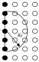
(a) (b) (c)

Fig. 2.4.1 Illustration of the influence domain for wall particles in (a) BC1, (b) BC2 and (c) BC3 (solid circle: wall particles; hollow circle: water particles)

To overcome the problem, Hibi & Yabushita (2004) and Zhang, Morita, Fukuda & Shirakawa (2006) suggested another method (referred as BC2). In the BC2, all the wall particles including outer layers are considered in solving the BVP for the pressure. In this implementation, the neighbouring particles of the wall particles in the first layer are distributed on both sides of the layer and therefore enhance the accuracy to some extent. When the pressure equation is applied to the first layer wall particles, the neighbours of the wall particles do not only include those on their right (water particles) but also those on their left (wall particles in other two layers as shown in Fig 2.4.1b). However, after doing so, the number of unknown pressure values is larger than the number of discretised equations. In order to obtain sufficient number equations, the pressure at wall particles in other two layers is related to the pressure at wall particles by assuming that the pressure is linearly distributed, e.g., the pressure at Particle J in Fig 2.4.1b is expressed as

) (

)

( _{I J I}

I

J _x x x

p p

p 

  

 (2.4.1)

where _x

I

U x

p_{  }

      

, U_xis the acceleration of wall with respect to x direction. It is noted that although the approximation to the pressure equation in the BC2 may be more accurate than that in the BC1, the problem about variation in the degree of approximation to the solid boundary condition still remain. That is, the spurious wiggles may also appear.

In both BC1 and BC2, the physical solid boundary condition is only approximately satisfied and sometimes wiggles in the time history of pressure are observed (Hibi & Yabushita 2004 and Sueyoshi & Naito, 2004a). Ma (2005a, b) employed another method to

I

Re

First layer Dummy particles

I J

Re

First layer Dummy particles

I

Re

35

implement the boundary condition, in which the pressure gradient for the wall particles in the first layer is forced to satisfy the physical solid boundary condition. This is referred as BC3 (shown in Fig. 2.4.1c). In the BC3, the solid boundary condition of pressure is directly applied to the wall particles in the first layer. That is, the discretised equation for them is based on the solid boundary condition. It could be understood that the approximation to the solid boundary condition in the BC3 depends less on the distribution of water particles and yields much smoother pressure.

Apart from these, Monaghan (1994) applied artificial force acting on the fluid particles near the solid boundaries. Lo and Shao (2002) suggested to use a mirror technique. But these methods mainly ensure the velocity to satisfy the solid boundary condition. Atluri (1998) solved the boundary value problems with a penalty method, the penalty method works well for fixed (or with little movement) boundary problems. As pointed out by Ma (2005a), the penalty method may cause unaccepted errors, particularly near the free surface.

2.5 Numerical methods for identifying the free surface

36

Different from the aforementioned methods, meshless methods discretize the fluid by particles. Hence it is a more natural way to track the free surface by following the free surface particles. In different meshless methods, there are different techniques to do so. For example, in the SPH methods, the free surface particles are identified by the density; i.e., if the ratio of the density of a particle to the fluid density is less than a specified value, such as 1%, it is then identified as a free surface particle [e.g., Lo and Shao, (2002)]. Khayyer et al. (2008c) compared the violent free surfaces using Incompressible SPH (CISPH) and Corrected Incompressible SPH (CISPH), and found that obvious improvements have been achieved for the judgements of the free surface by using the CISPH method. However, one can note that from the compared photographs shown in that paper, the thickness of the free surface (normally the thickness is one particle layer) was still thick especially in the breaking and post-breaking regions, which indicated that the efficiency of the technique of judging free surface in SPH methods is low.

In MPS method, one simple technique is used based on the following parameter

0 *

_/

_n

n

_I I





(2.5.1) where *

I

n is the particle number density at particle I as defined in Section 2.2.2.

37

38

3. MATHEMATICAL MODEL AND NUMERICAL METHOD

This chapter presents the governing equations, boundary conditions as well as the detailed the numerical procedures. The 2D and 3D MLPG_R formulations, including the numerical techniques for the domain integration, the gradient calculation scheme, are also presented.

Fig 3.0.1 shows the schematic of the computational domain and the coordinate system. The computational domain is chosen as a rectangle tank with a width of B. It may consist of two connected portions, the one with a flat seabed with a constant water depth of d and the other one with a sloping seabed with a sloping angle of . The lengths of these two portions are L1

and L2 respectively. The incident waves are generated by a wavemaker, which is mounted on the left side of the tank. A Cartesian coordinate system is used with the oxy plane on the mean free surface and with the z-axis being positive upwards.

Fig 3.0.1 Schematic of computational domain and the coordinate

3.1 Governing equations and boundary conditions

The fluid is assumed to be incompressible and governed by the continuity and momentum equations as follows:

0

 

 u （3.1.1）

L1 B d

Wavemaker z

x y

o

L2

39

u g

p Dt

u

D _ 1_{  }2_

 （3.1.2）

where

Dt

D _{is the substantial (or total time) derivative following fluid particles; u}_{is the fluid}

velocity, is the density of the fluid andpis the pressure, is the kinematic viscosity and g

is the gravitational acceleration.

The Lagrangian forms of kinematic and dynamic conditions on the free surface (z(x,y,t)) are given as followed

Dr u

Dt 



 _（3.1.3）

and

0

p （3.1.4）

where

r





xi





yj zk







is the position vector related to the origin of the coordinate system. The relative atmospheric pressure in Eq. (3.1.4) has been taken as zero. On the rigid boundary, the following kinematic and dynamic boundary conditions are satisfied:

U n u

n  (3.1.5)

and

   



 _{    } 

p n g n U n u

n_{. }     _  2

_(3.1.6)

where n is the inwards unit normal vector of the rigid boundary; U

and

U

are the

velocity and the acceleration of the rigid boundary, respectively.

3.2 Numerical Procedure

The mathematical model formed by Eqs. (3.1.1.) ~ (3.1.6) is solved by a time splitted scheme similar to Ma (2005a, b). Suppose the velocity, pressure and the location at nth _time

step are known, one can use the following numerical procedure to find them at (n+1)th _time

40

(1) Calculate the intermediate velocity (_u*_{) and position(r}*_{) of particles by using}

t u t

g u

u*_ n _ _{ }2n_{ （3.2.1）}

t

u

r

r



*

_



n

_



*

_

_(3.2.2)

where the superscript * and n represent the intermediate step and nth _{time step, respectively;}

t

 is the time step.

(2) Implicitly evaluate the pressure pn+1 _using

* 2

* 1 1

2 _{(1 ) u}

t t

p

n

n _

   

 





 _   _  _（3.2.3）

where



is an artificial coefficient between 0 and 1, and



n1 and



* are the fluid densities at (n+1)th _{time step and at the intermediate time step, respectively. For the}

incompressible flow, the density should be a constant and



n1=



, where



is the density of fluid specified initially. The density



* at the intermediate step may not be the same as



because the velocity and position calculated in Eqs. (3.2.1) and (3.2.2) do not necessarily satisfy the continuity equation given in Eq. (3.1.1).

(3) Calculate the fluid velocity and thus update the position of the particles using

1 *

*

_

_



t

_

_p

n

u





_（3.2.4）

1 *

* * *

1 



_

_

_

_



_

n

n

_u

_u

_u

t

_p

u









_（3.2.5）

t

u

r

r



n1

_



n

_



n1

_

_（3.2.6）

(4) Go to (1) for the next time step

41

method, may be adopted to solve this equation. But in this study, the MLPG_R method will be adopted.

In the meshless method, the computational domain is discretised by many particles. At each of the particles, a sub-domain is specified, which is a circle for 2D and a sphere for 3D cases. Eq. (3.2.3), after multiplying by an arbitrary test function, is integrated over the sub-domain, leading to





 



 _{ }

   

 

 

I I

I n

I

n _{u d}

t t

d

p      

 [ (1 ) *]

2 * 1 1

2  _(3.2.7)

where



_I is the area (2D problems) or volume (3D problems) of the sub-domain centred at particle I. Test function  can be chosen as different functions, which will lead to different formulations used in different meshless methods. For example, if



is defined as a Heaviside step function or a Rankine Source function, Eq. (3.2.7) will be changed to the governing equations used in the MLPG or MLPG_R methods (Ma, 2005a, b; Ma & Zhou, 2009; Zhou & Ma, 2010); or if



is defined as a



function, Eq. (3.2.7) will be the same as those used in the MPS method (Ikeda, 1999; Zhang, et al, 2005). The MLPG_R formulations for 2D and 3D will be detailed in the following subsection. Due to the facts that Rankine source function has different forms in 2D and 3D problems and that the integration domains of particles are also different in 2D and 3D problems, the MLPG_R formulations for 2D and 3D will be separately presented below for clarity.

3.3 MLPG_R Formulation for 2D cases

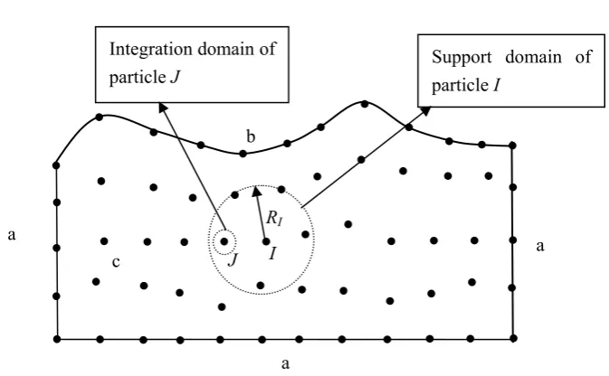
In the MLPG_R method, the particles are separated into three groups: those located on the rigid boundary (referred to as wall particles), those on the free surface (referred to as free surface particles) and others (referred to as inner particles), which are illustrated in Fig. 3.3.1. For each inner particle I, Eq. (3.2.7) is applied. The test function is taken as the Rankine source solution, i.e., the function  satisfies 20, in _I excluding the center and

0



42

)

/

ln(

2

1

I

R

r



[image:44.595.150.487.192.400.2]





(3.3.1) where r is the distance between a concerned point and the center of _I and R_I is the radius of _I.

Fig. 3.3.1 Illustration of particles, integration domain and support domain (a: wall particle; b: free surface particles and c: inner particles)

In Eq. (3.2.7), the second order derivative of unknown pressure and the gradient of the intermediate velocity are included. Numerical calculation of the derivative and gradient terms requires not only much computational time but also degrades the accuracy. In order to obtain a better form, Eq. (3.2.7) is changed, by adding a zero term _p2_{ and applying the Gauss’s}

theorem, into









                             























I I I I d u t dS u n t d t dS p n p n ] ) ( )[ 1 ( )] ( ) ( [ * * 2 *      (3.3.2)

where 



is a small surface surrounding the center of _I, which is a circle in 2D cases. The reason for adding 



is that the test function



in Eq. (3.3.1) becomes infinite at r=0

J I

RI

Integration domain of

particle J Support domain of _{particle I}

a

a a

b

43

and so the Gauss’s theorem can not be used otherwise. _n1_{in Eq. (3.2.7) has been replaced}

by a function of  based on the discusses below Eq. (3.2.3). One can easily prove that taking 0 results in (Ma (2005b))



         I dS p

n ( )] 0

[ (3.3.3)



     

 dS p p

n ( )]

[ (3.3.4)



        I dS u

n ( *) 0 (3.3.5)

and



    I I R d 4 2

 (3.3.6)

Using the results in Eqs. (3.3.3) ~ (3.3.6), Eq. (3.3.2) can be rewritten as:

           





   d u t R t p dS p n I I I I

I  _  _

 

 2 *

2 * ) 1 ( 4 ) ( 

 _(3.3.7)

where it has been assumed that the increment of the density (







*) is a constant within the sub-domain and so equal to its value at Particle I, which is acceptable not only because the density should not change much due to the change in the intermediate position of the particle but also because the small error caused due to the assumption is further reduced by multiplying the coefficient



that has a small value. The term may be evaluated in a more accurate way, for example by interpolation as done for the second term but such a way will not improve the accuracy significantly due to the reason.

It is obvious that Eq. (3.3.7) requires the intermediate density that is not computed in the MLPG_R method. Actually, the density can be replaced by a particle number density (PND) defined by Koshizuka and Oka (1996) in their MPS method as follows:



    N I j j I j

I W r r

n , 1

|)

44

where W is a weight function in terms of the distance between Particle I and Particle j, which becomes zero when the distance is larger than a certain value. The domain, within which the weight function is not zero, is called support domain (see the example shown in Fig. 3.3.1). In the above equation, N is the total number of particles in the support domain of particle I. As indicated by Koshizuka and Oka (1996), the PND is related to the density by:



 I V I I I I dV r W n m ) (



, (3.3.9)

where m_I is the mass of Particle I. The denominator of Eq. (3.3.9) is the integral of the weight function in the whole region VI, excluding a central part occupied by Particle I, this

integration is constant if the radius of the whole region VI is fixed. After applying Eq. (3.3.9),

Eq. (3.3.7) becomes

           





   d u t R n n n t p dS p n I I I

I _  _

 

 2 *

0 * 0

2 ₄ (1 )

)

( 

 _(3.3.10)

where _n0_{is the initial particle number density of fluid and} *

I

n is the particle number density of Particle I at the intermediate step. Ma (2005b) has detailed the method to discretize Eq. (3.3.10), in which the pressure on the left hand side is interpolated by a moving least square method (MLS) and the integration of the second term on the right hand side is evaluated by a semi-analytical technique. For the purpose of completeness, the details will be simply explained as follows.

3.3.1 Discretization of the governing equation for pressure

The unknown function p needs to be approximated by a set of discretized variable. Herein the approximation may be written as



   N J J J x p x p 1 ˆ ) ( )

(  (3.3.11)