Rigorous analysis of numerical methods: a comparative study

City, University of London Institutional Repository

Citation

:

Hada, S. L. & Rahman, B. M. (2016). Rigorous analysis of numerical methods: a

comparative study. Optical and Quantum Electronics, 48(6), 309.. doi:

10.1007/s11082-016-0579-x

This is the accepted version of the paper.

This version of the publication may differ from the final published

version.

Permanent repository link:

http://openaccess.city.ac.uk/17748/

Link to published version

:

http://dx.doi.org/10.1007/s11082-016-0579-x

Copyright and reuse:

City Research Online aims to make research

outputs of City, University of London available to a wider audience.

Copyright and Moral Rights remain with the author(s) and/or copyright

holders. URLs from City Research Online may be freely distributed and

linked to.

City Research Online:

http://openaccess.city.ac.uk/

[email protected]

Rigorous analysis of numerical methods: a comparative

study

Surendra L. Hada1•_{B. M. A. Rahman}2

Abstract For any photonic device simulation, the accuracy of the numerical solution not only depends on the methods being used but also on the discretization parameters used in that numerical method. In this work, Finite Element Method and Finite Difference Time Domain Method based on Maxwell’s equations were used to simulate optical waveguides and directional couplers. As the solution accuracy may also depend on the index contrast used in such photonic devices, the characteristics of low-index contrast Germanium doped Silica and high-index contrast Silicon Nanowire Waveguides were analyzed, evaluated and benchmarked. Numerical results to benchmark Directional Couplers are also reported in this paper.

Keywords Waveguides, couplers, and arraysFinite element methodsIntegrated optics

1 Introduction

The propagation of light through optical guided wave devices can be characterised by using various modelling techniques. These techniques can be classified into analytical methods and numerical methods. Analytical methods, if possible, a solution may be

1 _{Kathmandu University, Dhulikhel, Kavre, Nepal}

obtained by solving the basic electromagnetic equations. In contrast, numerical methods are computational schemes or models that can be applied to a spectrum of problems by modifying the basic model to fit the problem. Be it an analytical or numerical, an accurate modelling of optical waveguides and devices is important.

However, due to the complex nature for modern optical devices, the use of analytical methods is restricted to only simple structures. Even for two-dimensional optical waveg-uide structures, analytical solutions are not possible and some approximations have to be made (Rahman and Agrawal2013). Instead, existing and improved numerical methods and techniques are receiving wider attention for modeling optical components and devices, such as the Method of Moments (MoM) (Garcia et al. 2002; Hagness et al. 1997), the Finite Element Method (FEM), Beam Propagation Method (BPM), Finite Difference Method (FDM), the Finite Difference Time Domain Method (FDTD) (Luebbers1994), the Transmission Line Modeling method (TLM), and the Time Domain Integral Equa-tion (TDIE) techniques (de Electroniagnetisnio et al.1992).

2 Theory

2.1 Wave equation

Modal analysis of optical waveguides implies the process of finding the propagation constants and the field profiles of all the modes that a waveguide can support. To obtain these propagation characteristics, solutions of the well-known Maxwell’s equations given below, are necessary along with the satisfaction of the associated boundary conditions (Rahman and Agrawal2013):

r EþoB

ot ¼0 ð1Þ

r HoD

ot ¼J ð2Þ

In an isotropic lossless medium with no sourceðJ¼0;q¼0Þ, with constant permeability

l¼l₀, by eliminating the magnetic flux density in and the electric flux density compo-nents for Maxwell’s Eqs. (1) and (2) can be written as:

r2_Eþk2_{E¼0 ð3Þ}

r2_Hþk2_{H¼0 ð4Þ}

where, the wavenumber,k(rad/m) is given as;

k¼xpffiffiffiffiffiffiffiffiffiffil₀ ð5Þ

Equations (3) and (4) are called Helmholtz wave equations (Ma¨rz1995) for homoge-nous media.

2.2 Analytical method

confinement, analytical solution is not possible. Marcatili’s Method was one of the first semi-analytical approximation methods developed for the analysis of buried waveguides and couplers (Marcatili1969). This method works well in the regions far from cut-off but does not provide a satisfactory solution close to cut-off region (Chiang1994).

Subsequently, the Effective Index Method (EIM) was proposed by Knox and Toulios in 1970 (Knox and Toulios1970) as an extension to the Marcatili’s method that became one of the most popular methods in the 1970s for the analysis of optical waveguides whereby the rectangular structure is replaced by an equivalent slab with an effective refractive index obtained from another slab. The disadvantage of this method is that it does not give good results when the structure operates near cut-off region. However, the simplicity and speed of the method have encouraged many researchers to search for different approaches to improve the accuracy of the EIM, which subsequently led to many different variants of the EIM to be developed including the EIM based on linear combinations of solutions (Chiang

1986) or the EIM with perturbation correction (Chiang et al.1996).

2.3 Numerical methods

On the other hand, the Finite Difference Method, Finite Element Method, Beam Propa-gation Method, and the Finite Difference Time Domain Method are the popular numerical analysis methods used in many Engineering simulations. With continuous improvement of computational power at a reduced price, made these numerical methods more versatile, accurate and cost-effective.

2.3.1 Finite difference method

2.3.2 Finite element method

The Finite Element Method (FEM) is a numerical technique for solving a wide variety of engineering problems, including computational electromagnetics.

In FEM formulation, the domain of interest is divided into many discrete elements, often triangular, which is also the principal characteristic of the method. Each element is then possible to have different material properties in terms of its relative permeability and relative permittivity, thus making the dielectric material lossy, anisotropic, or non-linear, if necessary.

The accuracy of the method also depends upon the mesh, although a finer mesh across the whole domain may yield accurate results but at the cost of increased computing time. A finer mesh can be used in areas, where the field will have a rapid variation and/or higher magnitudes and a much coarser mesh in those areas where there is little variation or negligible field. Elements should not contain physical boundaries, i.e., there should be no abrupt change in property (e.g., refractive index) within the confines of an element even though the property may change from element to element. Symmetrical domains should have symmetrical meshes as well, although whenever possible it may be better to take advantage of the symmetry in the waveguide by using the appropriate boundary conditions along the line of symmetry. The variational procedure is applied to this functional by the way of the stationary requirement, from which the Euler equation is derived and which corresponds to the wave equation. We have used a magnetic-field based formulation as shown in Eq. (6), which is then integrated over the domain (Rahman and Davies1984).

x2_¼

R

ðr HÞ^1 _{ðr HÞdX}

R

Hl^HdX ð6Þ

where, xis the angular frequency of each waveguide mode,X is the waveguide cross-section and,^andl^are the permittivity and permeability tensors of the loss-free material, respectively.

The Rayleigh-Ritz approach can be applied to this (variational) formulation by using an interpolation function of the elements used to discretise the domain. The polynomial function, which approximates the field, should remain unchanged under a linear (or higher order) transformation form one co-ordinate system to the other. All the element contri-butions should then be combined to form a global matrix. The resultant system of (matrix) equations or rather matrix eigenvalue equation given in Eq. (7) (Rahman and Davies

1984), should be solved using an appropriate matrix solver, as the matrices are generally very sparse.

½Afxg k½Bfxg ¼0 ð7Þ

where, [A] is a complex Hermitian matrix and [B] is a real symmetric and positive-definite matrix,kis the eigenvalue and this can be taken ask2

0orb

2_{depending on the formulation}

used. However, for a loss-less optical waveguide, by consideringHz90out of phase with

the transverse components, the [A] and [B] matrices can be transformed to Real and Symmetric and its solution would then be easier.

2.3.3 Beam propagation method

light propagation in longitudinally varying wavguides such as tapers, Y-junctions, and bends. The beam propagation method was first applied to optoelectronics in 1980 (Feit and Fleck1980) and the solutions for the optical waveguides can be made to generate mode-related properties such as propagation constants, relative mode powers and group delays with high precision and considerable flexibility. The first reported BPM was based on the Fast Fourier Transform (FFT) and only solved the scalar wave equations under paraxial approximation. Therefore the FFT-BPM is only suitable for the case of weakly guiding structures, neglecting the vectorial properties of the field. Several numerical algorithms to treat the vectorial wave propagation (vector BPM) using the finite difference method, have been reported (Chung et al.1991; Huang et al.1992a; Huang and Xu1992b). The VBPMs are capable of simulating polarized or even hybrid wave propagation in strongly guiding structures. Subsequently, the finite element method has been utilised to develop BPM approaches. A unified finite element beam propagation method has been reported (Tsuji and Koshiba1996) for both TE and TM waves propagating in strongly guiding longitu-dinally varying optical waveguides. Obayya et al. (2000) has reported a full-vectorial BPM algorithm based on the finite element method to characterise 3-D optical guided wave devices.

Although imaginary distance BPM (Obayya et al.2000) can find modes in a uniform optical waveguide, but being a 3-dimensional method, these are numerically costlier than 2-D FDM or FEM based modal analysis approaches.

2.3.4 Finite difference time domain method

However, if the optical structure contain strong discontinuity or nonlinearity or time dependent excitation, a time-domain approach would be necessary.

Kane Yee published the first paper in May 1966 to describe Maxwell’s equations in the equivalent set of finite difference equations, thus showing the discretisation of space and time (Yee1966). This led to further investigation of time-varying media and also formed the basis of the Finite Difference Time Domain (FDTD) method. Yee’s approach applies a simple, second order accurate central-difference approximations for the space and time derivatives of the electric and magnetic fields directly to the respective differential oper-ators of the curl equations. The algorithm proposed by Yee solves for both electric and magnetic fields using the coupled Maxwell’s equations instead of solving individual components (electric or magnetic) alone with a wave equation, which is similar to the combined-field integral equation of the Method of Moments. Thus, creating a more robust solution in a straight forward manner in which the electric and magnetic properties of the material can be modeled. This method divides the three-dimensional geometry into cells to form a grid, called Yee cell.

Lewy factor, is then essential to minimise numerical instability, numerical dispersion and the numerical phase-velocity discontinuity. This stability factor for three dimensional geometry is then given by Taflove and Hagness (2005),

S¼cDt

ffiffiffiffiffiffiffiffiffiffiffiffiffiffiffiffiffiffiffiffiffiffiffiffiffiffiffiffiffiffiffiffiffiffiffiffiffiffiffiffiffiffiffiffiffi

1

ðDxÞ2þ

1

ðDyÞ2þ

1

ðDzÞ2

s

ð8Þ

where,cis the wave propagation speed,Dtis the time step,Dx,DyandDzare the space increments in the x, y and z directions, respectively, and the stability condition as,S\1. Although FDTD is a very powerful numerical approach but being a 4-dimensional approach (with added time), it is numerically much more expensive than the methods described earlier.

3 Numerical results

3.1 Benchmarking

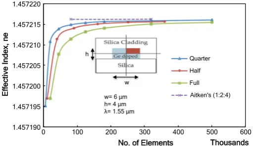
To consider a low-index contrast structure, first a waveguide with Germanium doped Silica core is studied, where cladding is pure Silica with refractive index of 1.44427. The core width is set at 6lm and height at 4lm. The index difference of the core with the cladding is considered to be 1.5 %, which enables us to investigate the behaviour of a low index contrast material. Using the H-field FEM (Rahman and Davies 1984), the numerical analysis has been carried out to find the effective index of the fundamental mode with different mesh divisions. The waveguide structure is simulated as a full waveguide and also exploiting onefold symmetry and twofold symmetry. The simulations are carried out at 1550 nm operating wavelength.

Figure1shows the variation of effective index with the number of elements being used for theH₁₁y mode. Here, effective index is defined as the ratio of propagation constant,b, to the wavenumber,k. It can be clearly observed that the effective index increases with the increase in number of elements to a certain level and then settles asymptotically. Initially,

1.457190 1.457195 1.457200 1.457205 1.457210 1.457215 1.457220

0 100 200 300 400 500 600

Effective

Index,

ne

No. of Elements Thousands

Quarter

Half

Full

Aitken's (1:2:4) w= 6 µm

h= 4 µm = 1.55 µm

w h

simulation was conducted for full waveguide structure and the result of the effective index is shown by a green line. As often there may be a limitations on the number of elements that can be used or computational resources needed, it should be noted that, if a structure has onefold or twofold symmetry, then this symmetry can be exploited. In this case, to show the advantages of exploiting symmetry, results for both the cases are also shown in Fig.1. As such, the effective index obtained for half symmetry is higher than that of full structure, shown by a red line. This shows that for a given number of elements, results using onefold symmetry is more accurate than that of considering the full structure. Similarly, in case of a twofold symmetry, it is even higher, shown by a blue line in this figure, compared to the other two lines. This clearly proves that whenever symmetry condition(s) exists, this can be exploited to improve the solution accuracy.

It should also be noted, sometimes several modes can have the same or very close eigenvalues. In that case, these modes can degenerate and eigenvectors can be mixed up. If symmetry condition is available, and used, mode degeneration can be avoided.

It is known that various extrapolation techniques can also be used to improve the solution accuracy further. Amongst them, Aitken’s extrapolation is a powerful one but this requires 3 successive solutions using a fixed geometric ratio of the mesh refinements, as given below (Rahman and Davies1985).

x1¼xrþ1

ðxrþ1xrÞ2

xrþ12xrþxr1

ð9Þ

where,xr1,xr,xrþ1are the results for three successive mesh refinements, andx1, is the

extrapolated result.

To test the convergence, the results obtained from twofold symmetry is used in Eq. (9), considering the mesh division ratio of 1:2:4. The result obtained is shown by the purple dotted line in Fig.1. In order to benchmark our results, the commercially available packages, COMSOL, FIMMPROP and the FDTD based Lumerical have been used for the simulation of the same waveguide structure.

Table1shows the effective index of Ge doped Silica core for fundamental quasi-TE,

H11y mode. The effective indices obtained using COMSOL, FIMMPROP, Lumerical and

the Aitken-extrapolation method are also tabulated in Table1.

The result shows effective indices are accurate upto the 5th decimal, for most of the approaches used here. The normalised propagation constant, ‘b’ variation with mesh size for Germanium (Ge) doped Silica is much less with 0.001 only, where ‘b’ is given by Marcatili (1969),

b¼ðneÞ 2

ðnsÞ2

ðngÞ2 ðnsÞ2

ð10Þ

where,neis the effective index of the waveguide, andnsandngare the refractive indices of

Silica cladding and the doped-Silica core, respectively.

Table 1 Effective index of Ge doped silica using various numerical methods

FEM (quarter structure)

Aitken’s COMSOL FIMMPROP Lumerical

Most of the optical waveguides are open-type structure and not confined inside a box. However, all the numerical method considers a finite computational region for analyses and at the computational boundary an artificial boundary condition is introduced depending on the natural boundary condition of the formulation used. These boundary conditions can be classified as (Itoh1989),

/¼0Homogenous Dirichlet ð11Þ

/¼kInhomogeneous Dirichlet ð12Þ

o/

ot ¼0Homogenous Neumann ð13Þ

where,/can be electric or magnetic field andkis a prescribed constant value. The vector

H-field formulation described in Eq. (6) has the natural boundary condition of an electric wall, i.e.nH¼0, where,nis the unit vector normal to the surface. Therefore, when this formulation is used, there is no need to force any boundary condition on conducting guide walls.

Earlier a powerful approach, infinite element was introduced to extend the domain of the field representation (Rahman and Davies1984). So, it is important to study the effect of using infinite element in which the computational domain can be extended in both the transverse directions.

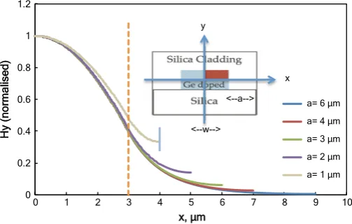
Figure2shows theHyfield variation along the x-direction without infinite element. The

Hy field variation obtained so far for the different waveguide width is converted to a

normalised form to compare them easily. Here, ‘a’ is shown as the distance of the right hand side boundary from the edge of the guide. When ‘a’ is reduced, Electrical wall comes closer to the waveguide core and influences the modal field. ForHy

mn mode, the vertical

metal (electric) wall imposes Neumann boundary condition on the dominantHy field. The

field plots in Fig.2show the case of Neumann boundary condition withoHy/ox=0 at the

computational wall. The introduction of metal wall on the side is equivalent to a multicore periodic waveguide array. In this case, (forH₁₁y mode), as the electric wall introduces

even-0 0.2 0.4 0.6 0.8 1 1.2

0 1 2 3 4 5 6 7 8 9 10

Hy

(normalised)

x, µm

a= 6 µm

a= 4 µm

a= 3 µm

a= 2 µm

a= 1 µm y

x

<--w--> <--a-->

like supermode field profile, so introduces error in mode profile and this also cause the effective index to increase as shown in Fig.3.

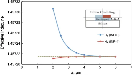
Figure3shows variation of effective index with respect to the distance,a, the distance between the waveguide core edge to the boundary wall of the computational domain, with and without infinite element. The blue line in the graph represents the effective index variation without infinite element, whereas, red line with the infinite element. In this case, effective index variation is more stable with the infinite element, even though the boundary wall is brought much closer to the core, compared to that of without infinite element as the percentage change in such variation is very less. It is being observed that Dn without infinite element is 0.0062856 %, whereas, with infinite element is 0.0002745 % only.

When infinite element is not used, the boundary wall acts like an electric wall. Hence, the effect of this wall is like a mirror, whereHy field is normal to this wall and forces a

non-zero value which mimics an even coupled array. As even supermode of a coupled structure has higher effective index than that of isolated modes, so here the effective index becomes higher than that of the actual mode. Similarly, if the boundary on the top and bottom come closer to waveguide, this will forceHy¼0 at the boundary and the effective

index of Hy₁₁ mode will reduce, as it mimics odd supermode. For the quasi-TM ðHx mnÞ

mode, the boundary condition of theHxfield would be Neumann for the upper and lower

boundary and Dirichlet for vertical side walls.

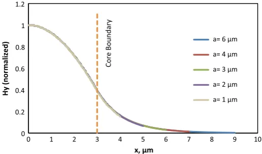
Figure4shows theHy field variation along the x-direction with infinite element. Once

again, theHyfield variation obtained so far for the different waveguide width is converted

to a normalised form to make them comparable with each other. The plot shows that the field, even when the side wall was closer to waveguide, still follows the actual modal field with highest waveguide width. That means, even when the computational domain is reduced, it does not force the natural boundary condition at that position. Resulting fields correctly represent the field decayðeax_{Þ in the cladding region.}

Next, a high-index contrast waveguide structure is considered, where a Silicon core, with refractive index of 3.47638, is placed on a SiO2 buffer having refractive index of

1.44427 and covered with Air cladding. The core width is taken as 800 nm and its height as 200 nm. Using the H-field FEM (Rahman and Davies1984), the numerical analysis has been carried out to find the effective index of the fundamental and second modes, for different mesh divisions. The structure considered here has an onefold symmetry. So, only

1.45720 1.45722 1.45724 1.45726 1.45728 1.45730 1.45732

0 1 2 3 4 5 6 7

Effective

Index,

ne

a, m

Hy (INF=0)

Hy (INF=1) <--a-->

half symmetry waveguide is represented and the simulation is conducted at 1550 nm operating wavelength.

The simulation result reveals that effective index increases with the finer mesh to a certain level and then settles asymptotically to 2.5829386, as shown by a blue line in Fig.5. Similar as for low-index contrast, to test the convergence, Aitken extrapolation technique has been used, considering a fixed geometric ratio of 1:2:4 and 1:1.5:2.25 (integer 4:6:9). Thus, the new effective index is calculated using Eq. (9), shown by red dotted line for 1:2:4 and green dot for 4:6:9. Based on the results, it is observed that the convergence value is more accurate with the geometric ratio of 4:6:9 for a given final mesh division used. Although using a geometric ratio 4:6:9 is more restrictive in distributing mesh over the whole problem domain, but we have observed that this approach yields better convergence than using a simpler 1:2:4 geometric mesh refinement.

Table2shows the effective index of the fundamental quasi-TEHy₁₁mode for a Silicon Nanowire. For comparison purpose, the commercially available packages, COMSOL, FIMMPROP and FDTD based Lumerical were used to find the effective index of the same

Fig. 4 Hyfield variation along width of waveguide for Ge doped Silica with infinite wall

2.573 2.574 2.575 2.576 2.577 2.578 2.579 2.58 2.581 2.582 2.583 2.584

0 500 1000 1500 2000 2500

Effective

Index,

ne

No. of Elements Thousands

Effective Index Aitken's (1:2:4) Aitken's (4:6:9) w= 800 nm

h= 200 nm = 1.55 µm

waveguide. The results shows effective indices are nearly close to each other with FIMMPROP result slightly higher and that of Lumerical considerably lower, which are also tabulated in Table2. It can be noted that for this case, when the index contrast is higher, variations of effective index with the mesh or between the approaches are higher than that of a low index contrast Silica guide, as shown in Table1.

However, as the Dn between the core and cladding index was higher for a Silicon nanowire, it may be useful to compare the range of normalized propagation constant,

b. The normalised propagation constant, ‘b’ variation with mesh size for Silicon Nanowire is also found to be significantly high with 0.0045. This suggests, extra care must be taken to find accurate solutions of high index contrast waveguides.

3.2 Directional coupler

The directional coupler is a key optical devices where modal solution can also be applied, and yet z-dependence optical parameter extracted from different numerical approaches can be tested. It works on the principle that the two guides, having separation,s, and with light input into Guide 1 is completely coupled into Guide 2 when the length of the device,Lc, is,

Lc¼

p

b_eb_o ð14Þ

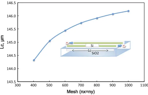
where,b_e andb_o are the propagation constants of the even and odd supermodes. UsingH-field FEM, the simulation of Silicon waveguide directional coupler was per-formed considering different width, height and separation ranging between 100 and 1000 nm. For these dimensions, simulation has been conducted for 400400 to 1000

1000 mesh divisions in order to analyse its trend. Typical result for the coupling length of the Silicon waveguide directional coupler for 800 nm core width, 200 nm core height and 100 nm separation for 1550 nm operating wavelength, with mesh division of 10001000 is found to be 146.19lm that seems to converge with very little increment if the simu-lation is carried out beyond 10001000 mesh. For the H-formulation used here, the individual propagation constants,be andbo of the two supermodes increase slightly with

the mesh, but their difference is more stable with the mesh division. The coupling length variation against mesh division is shown in Fig.6, which shows its convergence as the mesh number is increased. However, their differences reduces slightly, so with the increasing mesh,Lcincreases upto the saturation level.

Using commercial package, COMSOL, FIMMPROP and FDTD based Lumerical, the simulations were carried out for the Directional Coupler with the same physical dimension as above. Results show that the coupling length obtained from COMSOL and FIMMPROP were very close to the FEM results but slightly lower in case of Lumerical. The results are tabulated in Table3.

Table 2 Effective index of Si nanowire using various numeri-cal methods

FEM (half structure)

Aitken’s COMSOL FIMMPROP Lumerical

4 Conclusion

The Finite Element Method and Finite-Difference Time-Domain Method are very popular today in terms of solving electromagnetic problems. However, new codes, packages or methods are constantly published with novel analytical methods to solve electromagnetic problems. For any photonics modelling, it is useful to have some confidence in the results obtained.

In this paper, we aimed to provide a detailed and comprehensive analysis defining the modal characteristics of both low-index contrast Silica and high-index contrast Silicon nanowire waveguides and these are presented here. We have also shown the effects of the mesh size used and the infinite element. The results obtained so far are again compared with various other numerical methods in order to benchmark them. It can be noted that, as the solution accuracy of high index guide is slightly poorer, convergence of the modal solutions should be checked and if possible they should be benchmarked against another alternative approaches.

It is also shown the advantage of exploiting the structural symmetry, if available, to obtain better accuracy and also to avoid mode degeneration. Similarly, more accurate solution can be obtained by using Aitken’s extrapolation. Most of the commercial package do not clearly state the boundary conditions at the orthodox boundary, and it is shown here that if the boundary is taken close to waveguide core it can introduce error in both the effective index value and for the field profile. If possible, infinite element can be introduced to avoid artificial effect of the computational window. It should be noted that PML boundary (Berenger1994) should only be used when leakage or bending loss needs to be

Fig. 6 Variation of the coupling length with the mesh division

Table 3 Coupling length,Lc,

using various numerical methods FEM COMSOL FIMMPROP Lumerical

calculated, as introduction of PML makes the eigenvalue equation complex, and needs more computational resources.

Acknowledgments Authors acknowledge, numerical simulations by Dr. Ajanta Bahr, IIT Delhi, India, Mr. Jitendra K. Mishra, ISM, Dhanbad, India, Mr. Yousaf Omar Azabi, City University London, UK, Md. Enayetur Rahman, City University London, UK, and Mr. James Pond, Ph.D., Lumerical Solutions, Inc., Canada.

References

Berenger, J.P.: A perfectly matched layer for the absorption of electromagnetic waves. J. Comput. Phys.

114(2), 185–200 (1994)

Bierwirth, K., Schulz, N., Arndt, F.: Finite-difference analysis of rectangular dielectric waveguide

struc-tures. IEEE Trans. Microw. Theory Tech.34(11), 1104–1114 (1986)

Chiang, K.S.: Analysis of optical fibers by the effective-index method. Appl. Opt.25(3), 348–354 (1986) Chiang, K.S.: Review of numerical and approximate methods for the modal analysis of general optical

dielectric waveguides. Opt. Quantum Electron.26(3), S113–S134 (1994)

Chiang, K.S., Lo, K.M., Kwok, K.S.: Effective-index method with built-in perturbation correction for integrated optical waveguides. J. Lightwave Technol.14(2), 223–228 (1996)

Chung, Y., Dagli, N., Thylen, L.: Explicit finite difference vectorial beam propagation method. Electron. Lett.27(23), 2119–2121 (1991)

Davies, J.B., Muilwyk, C.A.: Numerical solution of uniform hollow waveguides with boundaries of arbitrary shape. In: Proceedings of the Institution of Electrical Engineers, vol. 113, pp. 277–284. IET (1966) de Electroniagnetisnio, G., de Cieiicias, F., de Granada, U.: Time-domain integral equation methods for

transient analysis. IEEE Antennas Propag. Mag.34(3), 15–23 (1992)

Feit, M., Fleck, J.: Computation of mode properties in optical fiber waveguides by a propagating beam

method. Appl. Opt.19(7), 1154–1164 (1980)

Garcia, S.G., Lee, T.W., Hagness, S.C.: On the accuracy of the ADI-FDTD method. IEEE Antennas Wirel. Propag. Lett.1(1), 31–34 (2002)

Hagness, S., Taflove, A., Bridges, J.: Wideband ultralow reverberation antenna for biological sensing. Electron. Lett.33(19), 1594–1595 (1997)

Huang, W.P., Xu, C., Chaudhuri, S.K.: A finite-difference vector beam propagation method for

three-dimensional waveguide structures. IEEE Photonics Technol. Lett.4(2), 148–151 (1992a)

Huang, W.P., Xu, C.: A wide-angle vector beam propagation method. IEEE Photonics Technol. Lett.4(10),

1118–1120 (1992b)

Itoh, T.: Numerical Techniques for Microwave and Millimeter-Wave Passive Structures. Wiley, New York (1989)

Knox, R., Toulios, P.: Integrated circuits for the millimeter through optical frequency range. In: Proceedings of Symposium Submillimeter Waves, vol. 20, pp. 497–515. Polytechnic Press of Polytechnic Institute of Brooklyn (1970)

Luebbers, R.: Three-dimensional cartesian-mesh finite-difference time-domain codes. IEEE Antennas

Propag. Mag.36(6), 66–71 (1994)

Marcatili, E.A.: Dielectric rectangular waveguide and directional coupler for integrated optics. Bell Syst. Tech. J.48(7), 2071–2102 (1969)

Ma¨rz, R.: Integrated Optics: Design and Modeling. Artech House on Demand, Boston (1995)

Obayya, S.A., Rahman, B.M.A., El-Mikati, H.: New full-vectorial numerically efficient propagation

algo-rithm based on the finite element method. J. Lightwave Technol.18(3), 409–415 (2000)

Rahman, B.M.A., Agrawal, A.: Finite Element Modeling Methods for Photonics. Artech House, Boston (2013) Rahman, B.M.A., Davies, J.B.: Finite-element solution of integrated optical waveguides. J. Lightwave

Technol.2(5), 682–688 (1984)

Rahman, B.M.A., Davies, J.B.: Vector-H finite element solution of GaAs/GaAlAs rib waveguides. IEE Proc. J. Optoelectron.132(6), 349–353 (1985)

Taflove, A., Hagness, S.C.: Computational Electrodynamics. Artech House, Boston (2005)

Tsuji, Y., Koshiba, M.: A finite element beam propagation method for strongly guiding and longitudinally

varying optical waveguides. J. Lightwave Technol.14(2), 217–222 (1996)

Yee, K.S.: Numerical solution of initial boundary value problems involving Maxwell’s equations in