Spaceplane trajectory optimisation with evolutionary-based initialisation

Spaceplane Trajectory Optimisation with Evolutionary-Based Initialisation

Christie Alisa Maddock, Edmondo Minisci

Department of Mechanical & Aerospace Engineering University of Strathclyde

Glasgow G1 1XJ, United Kingdom

[email protected], [email protected]

Abstract— In this paper, an evolutionary-based initialisation method is proposed based on Adaptive Inflationary Differential Evolution algorithm, which is used in conjunction with a deterministic local optimisation algorithm to efficiently identify clusters of optimal solutions. The approach is applied to an ascent trajectory for a single stage to orbit spaceplane, employing a rocket-based combine cycle propulsion system. The problem is decomposed first into flight phases, based on user defined criteria such as a propulsion cycle change translating to different mathematical system models, and subsequently transcribed into a multi-shooting NLP problem. Examining the results based on 10 independent runs of the approach, it can be seen that in all cases the method converges to clusters of feasible solutions. In 40% of the cases, the AIDEA-based initialisation found a better solution compared to a heuristic approach using constant control for each phase with a single shooting transcription (representing an expert user). The problem was run using randomly generated control laws, only 2/20 cases converged, both times with a less optimal solution compared to the baseline heuristic approach and AIDEA.

I. INTRODUCTION

One forerunner for the next generation of space access vehicles are spaceplanes. Spaceplanes operate both as an aircraft, taking advantage of the atmosphere at low altitudes where, for example, air-breathing engines can be used along with lifting surfaces, as a rocket at higher altitudes where the atmosphere is less dense, and as a spacecraft in orbit. This concept offers mass savings due to air-breathing engines, which reduces the need for on-board oxygen, and allow more control into the flight path and therefore the orbits that can be reached from a given take-off and landing site as well as a wider choice in the site, or spaceport, itself.

While a single stage to orbit offers full re-usability of the vehicle, it is still largely in the development stage, with many of the key technologies still unproven and also comes with a cost of lower payload fraction [1]. Reaction Engines’ Skylon vehicle is currently under research and development, with a proposed test flight in 2025. Multi-stage spaceplanes offer a more immediate time to market though often at a cost of partial expendability of parts. Virgin Galactic and S3 SOAR are two examples which use a carrier subsonic aircraft to launch a smaller spaceplane. Orbital ATK Pegasus is a multi-stage rocket launched from an aircraft that has been operational since 1990s.

From a design point of view, these vehicles are highly complex systems operating across very different environ-ments from low-altitude subsonic flight to high thermal loads during high altitude re-entry, to orbital insertion and

de-orbiting manoeuvres in space. Coupled with changes in operation, such as switching from an air-breathing engine to a closed-intake rocket engine or vehicle stage separations, the software models must be designed to handle discontinuities. The design of spaceplane mission delivering a payload to a specified orbit and re-entering is in itself a multiphase problem. Across the entire mission, assuming a returnable vehicle, the division is similar to an aircraft with runway take-off, ascent, operations (e.g., payload delivery), re-entry and runway landing. The two transatmospheric trajectories can be further divided in multiple segments; the elements defining the problem can differ though disciplinary models (e.g., propulsion modes for a hybrid engine, or in a multi-stage propulsion system), problem objectives and constraints, and level of fidelity needed within the models. To allow such flexibility in the design, the simulation needs to be structured in multiple phases, with interchangeable disciplinary models, plus mission objectives and constraints. The approach herein has been designed to allow each phase to define the set of models used and all the variables involved in the parametri-sation of the controls and propagation of the trajectory. The continuity between phases is guaranteed at convergence of the optimisation process by the optimiser and the problem formulation through constraints functions.

The development of methods presented here are part of a larger initiative to develop an integrated, multi-disciplinary design platform for quickly assessing and optimising con-ceptual vehicle design and performance for future space access vehicles, in particular single and multi-stage reusable vehicles. The trajectory optimisation solves for an open loop control scheme using a multi-phase approach for the configu-ration implemented with a direct multi-shooting transcription method. A set of first guesses are generated using the in-house Adaptive Inflationary Differential Evolution (AIDEA) algorithm [2], which focuses on exploration, followed by a local optimisation of candidate solutions using a derivative based method for non-linear, constrained problems using a fixed time step integrator. The trajectories are then re-propagated with the locally optimal control laws using a variable step numerical integrator with lower tolerances (higher accuracy) to ensure the feasibility of the solutions. The results for the first guess using AIDEA are compared against a phase-based single shooting method using an user supplied control law based on educated guessing.

a payload delivery mission to a 100 km altitude, circular, equatorial orbit. The objective function is the maximisation of the payload mass delivered to an orbit, with equality constraints on the final position and velocity vectors. Using AIDEA for the first guess generation has proved robust and effective at finding sets of feasible, locally optimal solutions which can be used to understand the trade-offs between performance and vehicle design.

II. OPTIMISATION APPROACH

The optimisation algorithms and approach are shown below, describing the transcription method, based on direct multi-shooting transcription and flight mission decomposi-tion, the evolutionary-based initialisation using AIDEA, and the local derivative-based optimisation and refinement step.

A. Transcription

The optimal control problem is transcribed into an nonlin-ear programming problem by using a multi-phase, multiple-shooting approach. The mission is initially divided into np user-defined phases. Within each phase, the time interval is further divided intonmultiple shooting segments.

∪np k=1∪

n−1

i=0 [ti,k, ti+1,k] (1) With each interval[ti,k, ti+1,k], the control is further discre-tised intonc control nodes{ui,k0 , ..., ui,knc}and collocated on

Tchebycheff points in time.

Continuity constraints on the control and states are im-posed,

xi,k=F([ti−1,k, ti,k],xi−1,k)

ui−1,k nc =u

i,k

0

for k= 1, ..., np (2)

x1,k=x(tn+1,k−1)

u1₀,k=un+1,k−1

nc

fork= 2, ..., np (3)

where F([ti−1,k, ti,k],xi−1,k) is the final state of the nu-merical integration on the interval [ti−1,k, ti,k] with initial conditions xi−1,k. This approach increases the degree of freedom of the optimisation process reducing the sensitivity of the overall problem to its variables although at a cost of a steep increase in the number of optimisation variables.

The optimisation variables are therefore:

• The initial state vector of each shooting segment within every phase (excluding the first segment of the first phase)xi,k

• The control nodes of each shooting segment

{ui,k₀ , ...,ui,k nc}

• The time of flight for each shooting segment ∆ti,k The discretised optimisation problem is defined as

min {ui,k_j },{xi,k},{∆ti,k}

φ(xn,np) + np

X

k=1

n−1

X

i=0

∆ti,kf0(xi,k,ui,kj ) (4)

subject to

xi,k=F([ti−1,k, ti,k],xi−1,k),

ui_n−1,k

c =u

i,k

0 ,

x1,k=x(tn+1,k−1),

u1₀,k=un_n+1,k−1

c ,

c(x(t), u(t))≤0, t∈[t0, tf] g(xn,k,un,knc )≤0,

ω(x0,1,xn,np) = 0

for i= 1, ..., n−1,k= 1, ..., np and∆ti,k =ti+1,k−ti,k. Path constraints are evaluated at a discrete set of points based in time, andg(xn,k,un,knc )are the inequality constraints for

phase switching.

The resulting optimisation problem is usually handled via standard derivative-based methods, requiring a trial-and-error approach by an knowledgeable or expert user to find a suitable starting point, i.e., an initial solution that can produce a near-feasible solution that will allow the local deterministic optimiser to converge. In this respect, the possibility to use evolutionary algorithms to find a suitable starting point is explored in this paper. Using an evolutionary approach also has the benefit of producing multiple first guesses as well as clustering information on the archived solution sets.

B. Adaptive Inflationary Differential Evolution Algorithm

The creation of the algorithm stemmed from the idea to create new hybrid algorithms that take elements from different approaches and use them as building blocks for a new algorithm. Following this approach, one of the co-authors [3] first co-proposed the Inflationary Differential Evolution Algorithm (IDEA) in 2011, which combines dif-ferential evolution (DE) [4] with the restarting procedure of Monotonic Basin Hopping (MBH) [5] algorithm. IDEA showed very good results when applied to problems with a single or multi-funnel landscape. However, its performance was found to depend on the parameters controlling both the convergence of DE and MBH, and the inflationary stopping criterion used to terminate the DE search. In particular, the DE performance is strongly influenced by the crossover probability CR and the differential weight F whose best settings are heavily problem dependent [6]. This led to the development of Adaptive-IDEA, or AIDEA, which uses a probabilistic, Parzen-based kernel approach to automatically adapt the values of bothCRandF during the search process [2]. Tested on several engineering problems, AIDEA showed both good exploratory and local search performance, making it a suitable approach for the initialisation of spaceplane trajectories.

The general procedure for the AIDEA used in this paper is:

2) Then the joint PDF forCRandF,CRFp, is initialised to be a uniform distribution. At this point, the actual optimisation loop starts by sampling the two vectors

CRk andFk, where kis the current iteration. 3) DE is run drawing probabilistically a value forF and

CR from CRFp, and CRFp is updated on the basis of the improvement of the individual using the drawn values of F andCR.

4) At this point,

a) if the population contracts below the predefined threshold, a local optimiser from current mini-mum is run, and at the end of local optimisation, b) if the local optimiser failed to improve the value offminmore thaniunmaxtimes, the population is restarted globally andiunis set to0, otherwise, the population is restarted within a local bubble andiun=iun+ 1.

5) At this point,

a) if the population is re-initialised, the loop restarts from the initialisation ofCRFp,

b) otherwise just the DE loop restarts.

6) As a terminal criterion, the algorithms stops if the maximum number of function evaluations,nf eval,max, has been performed.

In particular, the initialisation of theCRFpto an uniform distribution is done by building a regular mesh with (nk+

1)×(nk+ 1)points (wherenk is a predefined value) in the space CR ∈[0.5,0.99]×F ∈[0.1,1]. Note, this approach and space definitions are different from the original AIDEA. A Gaussian kernel is then allocated on each node and the PDF is built by Parzen approach [7]. A step change value, ddis linked to each kernel (row ofCRFp) and its initial value is set= 0.npop values ofCRandF are sampled from the Parzen distribution and each couple of CR and F values is associated to one element of the population and used to create the offspring on the basis of the chosen strategy.

During the optimisation, the location of the kernels is updated on the basis of the obtained results. More in details, to update the matrix containing the location of kernel centres (CRFp) after that rows ofCRFp are sorted on the basis of the associated value of dd, if the objective function of the offspring has a value that is strictly lees then the parents (it is supposed a minimization problems) then the element of the sorted CRFp are sequentially evaluated and the first time that the associatedddvalue of the row is less than the difference between the objective function of the parent and that of the offspring then the F value used to operate on the individual xi,k substitutes the element CRFp,2,j,k. The CR value used to operate on the individualxi,k substitutes the elementCRFp,1,j,konly if the difference between parent and offspring is greater than a predefined threshold CRC. The different approach for updating the CR coordinate of the kernels is meant to dump the learning of the crossover to avoid the too fast convergence toward the extremes of the allowed range that can occur in some cases. Note that, as for other self-adaptive schemes, the adaptive version of IDEA

has an additional parameter to be adjusted: the threshold on the minimum expected improvement of the cost function. This threshold is used to limit the updating ofCR, a failsafe procedure that has proven to improve the robustness of the algorithm. For a complete description of the original algorithm, see [2], [8].

C. User Defined Constant Control Initialisation Procedure

A first guess solution can be generated based a phase-based single shooting method. A control scheme is defined by the user which are linearly interpolated within each phase. For the test case here, a constant set of controls are used for each phase. A set of event functions are set, based on optional user defined conditions, the upper and lower bounds for the states for each phase and the final state. When an event condition is triggered, the integration for that phase is stopped, with the final state from that phase used as the initial state for the next phase.

D. Evolutionary-based Initialisation Optimisation Proce-dure

1) As AIDEA can only handle unconstrained optimisa-tion problems, the constrained problem in (4) is first converted into an unconstrained one.

min {ui,k_j },{Ti,k}

φ(xn,np) + np

X

k=1

n−1

X

i=0

∆ti,kf0(ui,kj )

+wα

X

u

i−1,k nc −u

i,k

0

+wα

X

u

1,k

0 −u

n+1,k−1

nc

+wβ

X

ca+

X

ca+

X

ωa

(5)

whereware weights, andca,gaandωaare the active inequality constraints. Note that equality constraints enforcing matching of the state vectors between the segments is not considered as during the initialisa-tion phase the trajectory is propagated using single-shooting direct transcription approach (using the single shooting integration approach in Section II-C). 2) Within AIDEA, for each iteration of the underlying DE

the current, best solution is saved into an archiveAbest along with the best individual in the population found with a local search before a local or global restart is initiated.

3) At the end of a run of AIDEA, the final population is added to the archiveAbest.

4) All the solutions in the archive Abest are clustered on the basis of the Euclidean distance in the search space. The clusters are then ranked on the basis of the performance of best solution within the cluster, where the first cluster,Cbest,1, contains the overall best

solution found by AIDEA during that run.

III. SPACEPLANE SYSTEM MODELS

In this section, mathematical models are presented for the vehicle design and operation of a single-stage-to-orbit (SSTO) spaceplane. The models are divided by discipline: vehicle mass and configuration, aerodynamics and propul-sion, environment models for Earth including dimensions, gravitational field and atmospheric model, and the flight dynamics and control.

A. Vehicle Model

The model configuration is based on the CFASTT-1 con-ceptual test vehicle [9], which has a gross take-off mass of 260 tons. The design of the vehicle is similar in scale and function to Reaction Engines’ Skylon C1 SSTO vehicle [10], and was designed as an open test case to examine alternate vehicle configurations and aerodynamic properties.

B. Environment

The Earth is modelled as oblate spheroid based on the WSG-84 model. The gravitational field was modelled using 4th order spherical harmonics (accounting forJ2,J3 andJ4

terms) for accelerations in the radial gr and transverse gφ directions [11]. The angular rotation of the Earth is assumed constant atωE = 7.292115×10−5 rad/s.

The atmospheric conditions – temperatureTatm, pressure patm, density ρatm and speed of sound – are modelled through the global International Standard Atmosphere (ISA) model as a function of altitude.

C. Aerodynamics

The aerodynamic model of the vehicle predicts the total coefficient of lift cL and drag cD as a function of the angle of attack α and Mach number M(h, v). For the test case presented here, the aerodynamics were first run with higher fidelity simulations using CFD for the continuum regime (lower atmosphere) and Direct Simulation Monte Carlo based methods for the upper atmosphere [12] to obtain a set of discrete data points. These data sets were used to fit a set of polynomial-based surrogate models for cLα and

cD0. The net values for thecL andcD are then determined

based on linearised aerodynamic theory for the supersonic regime and modified Newtonian theory for the hypersonic regime, linked together through a bridging function. The drag coefficient is calculated as the sum of a CD0 term and the

induced drag of lifting surfaces (cLtanα). The lift L and dragD forces in the vehicle body reference frame are given by the equations,

L=cLρatmv

2_S

ref

2 D=

cDρatmv2Sref

2 (6)

where Sref is the total aerodynamic reference area of the vehicle, for this test caseSref = 300m2.

D. Propulsion

The propulsion system is assumed to be a rocket-based combine cycle engine with two distinct modes of operation, modelled as two different engines with an instantaneous switching mechanism.

The rocket cycle is modelled based on Tsiolkovsky rocket equations. The present configuration used in the test case uses LOX/LH2 rocket engines with anIspof 450 s. The fuel mixture ratio is assumed constant and the two propellants are treated as a single mass flow m˙p. A throttle control τ∈[0,1]is added, which dictates the fraction of maximum available thrust applied and fuel mass flow (and therefore consumption). A simplifying assumption is made that the mass flow varies linearly with thrust. The maximum total thrust in a vacuum is set at FT0,max = 4 MN. The instantaneous thrust and mass flow rate are then calculated as,

˙

mp=τ

FT0,max g0Isp

(7a)

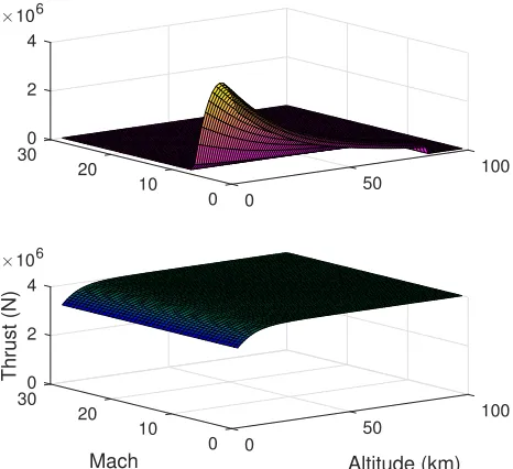
FT ,h=FT =τ(FT0,max−patmAe) (7b) A penalty proportional to atmospheric pressure patm and nozzle exit areaAeis introduced to account for the difference in nozzle expansion under pressure compared to in a vacuum. The air-breathing cycle was simulated using a higher fidelity tool designed for combined cycle engines [13], [14]. Due to the high computational overhead, a dataset was generated and used to fit a simpler analytic model. The model in (7) was used with a variable equation for the Isp as a function of altitude, Mach and throttle. The net thrust from the two models are show in Figure 1.

0 30 2

100

×106

20 4

50 10

0 0

0 30 2

100 ×106

Thrust (N)

20

Mach Altitude (km)

4

50 10

0 0

E. Trajectory Dynamics and Control

A 3-DOF variable point mass dynamic model is used where the spaceplane is a time-varying mass located at the centre-of-gravity of the vehicle. The state vector for the flight dynamics xdyn = [r, ˙r] is the spherical coordinates for the positionr= [r, λ, θ]and the velocity ˙r= [v, γ, χ]wherer is the radial distance,(λ, θ)are the latitude and longitude,v is the magnitude of the relative velocity vector directed by the flight path angle γ and the flight heading angle χ. The equation of motion is expressed in the Earth-Centred-Earth-FixedF rotating reference frame [15].

¨

r= F

F

m(t)−2ωE×r−ωE×(ωE×r) (8)

where the vehicle mass m(t) is a sum of the constant dry and payload masses, and the mass of the on-board propellant mp(t) =R_tm˙p dt,FF is net force from the lift L, drag D, gravitational forces in the radial and transverse directions

[mgr, mgφ] and propulsion thrust FT converted from the vehicle body reference frame based on the vehicle angle of attackαand bank angleµ.

FF=



 

FTcosαcosµ−D

m −grsinγ+gφcosγcosχ FTsinµ

m −gφsinχ FTsinαcosµ+L

m −grcosγ−gφsinγcosχ





 (9)

The thrust is assumed to be aligned to the x-axis of the vehicle body reference frame. The explicit equations for the dynamic model can be found implemented in [16], or more generally derived in [11].

The discrete control law is interpolated using piecewise cubic Hermite interpolating polynomial. Within the global and local optimisation, the trajectory dynamics are integrated using an non-adaptive 4th _{order Bogacki-Shampine} Runge-Kutta method. For the refinement, an adaptive Runge-Runge-Kutta 4/5 integrator is used with a tolerance of 10−9_.

IV. RESULTS

The proposed initialisation approach has been applied to solve the trajectory optimisation problem related to the ascent phase of the spaceplane, from transonic conditions at low altitude to low orbital boundary conditions. The outcome of the proposed method is compared to the results of the trajectory optimisation process with a single shooting initialisation.

A. Test Case

The test case is for a payload delivery mission to LEO. The objective function is to minimise the fuel consumption, mp, which is analogous to maximising the payload delivered to orbit assuming a fixed gross take-off mass for the vehicle, and therefore that the sum(mp+mpayload)is also fixed.

The problem is decomposed into two phases correspond-ing to the two propulsion modes: Phase 1 uses an air-breathing cycle, while Phase 2 uses the rocket cycle. Phase 1 is configured with n = 2 multi-shooting segments and

nc= 5control nodes per segment, while Phase 2 hasn= 4 andnc= 5.

Table I lists the initial and final boundary conditions, and the upper and lower bounds for the state and control vari-ables. The trajectory is designed to be within the equatorial plane, starting from a nominal position 0◦E longitude on the equator and ascending to a 100 km, circular equatorial orbit. The arrival true anomaly is left free, with the final altitude hf = 100 km, orbital velocity vf and flight path angle γf = 0◦ set as equality constraints. As the trajectory is in-plane, the control parameter for the bank angleµis set to 0.

B. User Defined Constant Control Initialisation

A trajectory obtained by using a single shooting approach per phase with user defined constant control laws has been used as first guess for the gradient-based optimisation of the control laws. For the first phase,α= 5◦andτ= 1, while the second phaseα= 20◦ andτ = 1. The optimisation process converges to a final fuel massmp = 189011 kg after 9013 model evaluations (∼1800 s on a CORE i5 CPU running Matlab 2016a).

C. Evolutionary Based Initialisation

For this test case, AIDEA is set with DE population size npop = 20, number of AIDEA local restarts iunmax =

5, δb = 0.1 where ±δb is added to current solution to create the local bubble for local restart, inflationary tolerance tolconv = 0.25, distance for global restart δc = 0.1, adaptation thresholdCRC= 3, and the adopted DE strategy was DE/best/1/bin (see [4]).

All reported statistics in Table II are computed on the re-sults obtained from 10 independent runs of AIDEA (multiple independent runs allows for the evaluation of the robustness of the method). It can be seen that for all the runs the method converges to a feasible solution, and on 40% of the cases the performance is comparable to, or better than, the solution obtained by user defined single shooting initialisation. The extra computational costs are offset by the robustness of the approach and the saving in required user expertise and trial-and-error time.

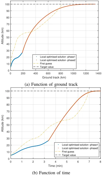
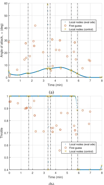
Figures 2–4 show the trajectory dynamics, vehicle mass time history and control law for the best solution in Table II. For the dynamics, Figs. 2–4 show the first guess found by AIDEA, the locally optimised solution divided by phases to show the optimised switching point for the propulsion mode, the refined solution and the target value. The controls in Fig. 5 show the control nodes for the AIDEA solution and the locally optimal solution, as well as the interpolated nodes used by the integrator within the local optimisation and the smoothed interpolation (pchip) used in the refinement integration step. The duration of each segment within each phase is also shown, as the time-of-flight for the segments were optimisation variables.

TABLE I: BOUNDARYCONDITIONS ANDBOUNDS ONSTATE ANDCONTROLVARIABLES

Variable Initial conditions Bounds per phase Final conditions

Phase 1 Phase 2

Altitude,h h0= 5km [0.8h0, 30] km [h0,1.2hf]km hf = 100km

Latitude,λ 0 deg N [−45,+45]deg N [−45,+45]deg N free Longitude,θ 0 deg E [−180,+180]deg E [−180,+180]deg E free

Relative velocity,v v0= 400m/s [0.5v0,1000]m/s [0.5v0,2vf] vf = 7381m/s

Flight path angle,γ 6 deg [−90,+90]deg [−90,+90]deg 0 deg Flight heading angleχ 90 deg [−180,+180]deg [−180,+180]deg free

Vehicle mass,m m0= 2.47×105 kg [mdry, mgtow] [mdry, mgtow] J= min(mp)

Angle of attack,α N/A [0,+40]deg [0,+60]deg N/A Engine throttle,τ N/A [0.8,1] [0.4,1] N/A Time of flight,∆t N/A [10,200]s [50,500]s N/A

with the engine cut-off (τ = 0) during the last segment creating a coasting arc. This means that the spaceplane also arrives at the target orbit the correct velocity vector and zero acceleration, which was not added as a constraint in order to evaluate the optimality of the solutions found.

No matching constraints were imposted between segments on the controls nor derivative limits on the control imposed (e.g., to limit dα/dt or to match u˙1₀,k = u˙n_f+1,k−1). For the most part, the controls are smooth with one exception producing an spike in α (Fig. 5a) between the second and third segments. Due to the close proximity in time to the two neighbouring points, the effect on the dynamics in negligible.

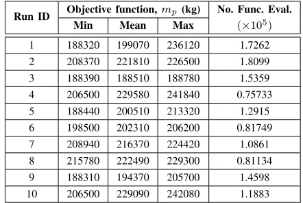
TABLE II: STATISTICS ON RESULTS FROM AIDEA INI-TIALISATION

Run ID Objective function,mp(kg) No. Func. Eval.

Min Mean Max (×105₎

1 188320 199070 236120 1.7262

2 208370 221810 226500 1.8099 3 188390 188510 188780 1.5359 4 206500 229580 241840 0.75733 5 188440 200510 213320 1.2915 6 198500 202310 206200 0.81749 7 208940 216370 224420 1.0861 8 215780 222490 229300 0.81134 9 188310 194370 205700 1.4598 10 206500 229090 242080 1.1883

D. Random Initialisation

To better understand the potentialities of the proposed method, 20 optimisation runs have been initialised by uni-form random sampling within the entire search space. Of the 20 runs only two processes converged to feasible results, with the objective function mp = [205870,200220] kg. The 20 runs had a total computational cost of6×105_function

evalu-ations. Even if the sampling cannot be considered enough for a correct statistical analysis of the process performance, the success rate of the process is∼0.1and near3×105_function

evaluations should be spent to have a feasible solution with

this approach on such a problem, compared to less than

1.2×105_{evaluations of the evolutionary based initialisation.}

V. CONCLUSIONS

This paper has introduced an evolutionary-based ini-tialisation using AIDEA followed by a local optimisation procedure to identify clusters of locally optimal solutions, applied to the multi-phase ascent trajectory of a hybrid propulsion spaceplane. The solutions found by this method were compared against a more conventional case using a first guess generated by with a constant control law per phase, and a random initialisation approach. The user defined constant control initialisation approach requires a degree of trial-and-error and a familiarly with the specific problem, meaning a high cost in terms of human time, while the random approach is computationally expensive. Instead, the AIDEA-based method requires less problem-specific inputs of the constant control initialisation approach, and is more efficient and more robust at finding a potentially globally optimal solution as well as highlighting clusters of locally optimal trajectories which can be used by the designer to understand the sensitivity of the optimisation variables (for example here, the propulsion switching point and control law) to the performance or mission objectives and constraints, than the random initialisation.

Future work will investigate better formulations of the problem handled by AIDEA, and to improve the robustness and the convergence properties of the gradient-based method. This approach will also be applied to more complex, longer duration test cases for future space access vehicles.

REFERENCES

[1] R. Varvill and A. Bond, “A comparison of propulsion concepts for SSTO reusable launchers,”Journal of the British Interplanetary Society, vol. 56, no. 3/4, pp. 108–117, 2003.

[2] E. Minisci and M. Vasile, “Adaptive inflationary differential evolution,” inIEEE Congress on Evolutionary Computation (CEC2014). Beijin, China, 2014.

[3] M. Vasile, E. Minisci, and M. Locatelli, “An inflationary differential evolution algorithm for space trajectory optimization,”IEEE Transac-tions of Evolutionary Computation, vol. 15, no. 2, pp. 267–281, 2011. [4] K. Price, R. Storn, and J. Lampinen,Differential Evolution. A Practical

0 200 400 600 800 1000 1200 1400 Ground track (km)

0 10 20 30 40 50 60 70 80 90 100

Altitude (km)

Local optimised solution -phase1 Local optimised solution -phase2 First guess

Target value

(a) Function of ground track

0 1 2 3 4 5 6 7 8

Time (min) 0

10 20 30 40 50 60 70 80 90 100

Altitude (km)

Local optimised solution -phase1 Local optimised solution -phase2 First guess

Target value

(b) Function of time

Fig. 2: Trajectory altitude showing the first guess from AIDEA, and the locally optimised solution for the two phases.

[5] B. Addis, M. Locatelli, and F. Schoen, “Local optima smoothing for global optimization,”Optimization Methods and Software, vol. 20, pp. 417–437, 2005.

[6] R. Gamperle, S. Muller, and P. Koumoutsakos, “A parameter study for differential evolution,” in WSEAS International Conference on Advances in Intelligent Systems, Fuzzy Systems, Evolutionary Com-putation, 2002, pp. 293–298.

[7] K. Fukunaga,Introduction to Statistical Pattern Recognition. Aca-demic Press, 1972.

[8] M. Vasile and V. Becerra, Eds., Computational intelligence in aerospace sciences, ser. Progress in Astronautics and Aeronautics. [9] F. Pescetelli, E. Minisci, C. Maddock, I. Taylor, and R. Brown, “Ascent

trajectory optimisation for a single-stage-to-orbit vehicle with hybrid propulsion,” inAIAA/3AF International Space Planes and Hypersonic Systems and Technologies Conference, 2012, p. 5828.

[10] R. Longstaff and A. Bond, “The Skylon project,”AIAA Journal, 2011. [11] A. Tewari,Atmospheric and space flight dynamics. Springer, 2007. [12] A. O. Ahmad, C. Maddock, T. Scanlon, and R. Brown, “Prediction of the aerodynamic performance of re-usable single stage to orbit vehicles,”Space Access, 2011.

[13] A. Mogavero, I. Taylor, and R. E. Brown, “Hybrid propulsion para-metric and modular model: A novel engine analysis tool conceived for design optimization,” in AIAA International Space Planes and Hypersonic Systems and Technologies Conference, 2014.

[14] A. Mogavero, “Toward automated design of combined cycle propul-sion,” Ph.D. dissertation, University of Strathclyde, Glasgow, UK, 2016.

[15] N. Vinh,Optimal trajectories in atmospheric flight. Elsevier, 2012, vol. 2.

[16] F. Toso, C. Maddock, and E. Minisci, “Optimisation of ascent

tra-0 1 2 3 4 5 6 7 8

Time (min)

0 1 2 3 4 5 6 7 8

Velocity (km/s)

Local optimised solution -phase1 Local optimised solution -phase2 First guess

Target value

(a)

0 1 2 3 4 5 6 7 8

Time (min) 0

5 10 15 20 25 30 35 40 45

Flight path angle (deg)

Local optimised solution -phase1 Local optimised solution -phase2 First guess

Target value

(b)

Fig. 3: Trajectory velocity and flight path angle showing the first guess from AIDEA, and the locally optimised solution for the two phases.

0 1 2 3 4 5 6 7 8 Time (min)

0 0.5 1 1.5 2 2.5

Vehicle mass (kg)

×105 Final mass: optimised 58570 kg, first guess: 43976 kg Local optimised solution First guess

Fig. 4: Variation of vehicle mass with time for AIDEA-initialised solution.

0 1 2 3 4 5 6 7 8

Time (min) 0

10 20 30 40 50 60

Angle of attack,

α

(deg)

Local nodes (eval ode) First guess Local nodes (control)

(a)

0 1 2 3 4 5 6 7 8

Time (min) 0.4

0.5 0.6 0.7 0.8 0.9 1

Throttle

Local nodes (eval ode) First guess Local nodes (control)

(b)