Classification of Power Quality Disturbances Using Wavelet Packet Energy Entropy and LS SVM

Classification of Power Quality Disturbances Using

Wavelet Packet Energy Entropy and LS-SVM

Ming Zhang, Kaicheng Li, Yisheng Hu

College of Electrical and Electronic Engineering, Huazhong University of Science and Technology, Wuhan, China E-mail: [email protected]

Received April 11,2010; revised May 22,2010; accepted June 27,2010

Abstract

The power quality (PQ) signals are traditionally analyzed in the time-domain by skilled engineers. However, PQ disturbances may not always be obvious in the original time-domain signal. Fourier analysis transforms signals into frequency domain, but has the disadvantage that time characteristics will become unobvious. Wavelet analysis, which provides both time and frequency information, can overcome this limitation. In this paper, there were two stages in analyzing PQ signals: feature extraction and disturbances classification. To extract features from PQ signals, wavelet packet transform (WPT) was first applied and feature vectors were constructed from wavelet packet log-energy entropy of different nodes. Least square support vector ma-chines (LS-SVM) was applied to these feature vectors to classify PQ disturbances. Simulation results show that the proposed method possesses high recognition rate, so it is suitable to the monitoring and classifying system for PQ disturbances.

Keywords:Power Quality (PQ), Wavelet Packet Transform (WPT), Wavelet Packet Log-Energy Entropy, Least Square Support Vector Machines (LS-SVM)

1. Introduction

The deregulation polices in electric power systems re-sults in the absolute necessity to quantify power quality (PQ). This fact highlights the need for an effective rec-ognition technique capable of detecting and classifying the PQ disturbances. Traditionally PQ recordings are analyzed in the time-domain by skilled engineers. How-ever, PQ disturbances may not always be obvious in the original time-domain signal. One of the traditional signal processing techniques called Fourier transform provides information in frequency-domain but it does have limita-tions. One crucial limitation is that a Fourier coefficient represents a component that lasts for all time. This makes Fourier analysis less suitable for non-stationary signals. Wavelet analysis, which provides both time and fre-quency information, can overcome this limitation. Unlike the Fourier transforms, the wavelet transform has a fully scalable window, which allows a more accurate local description and separation of signal characteristics [1]. The wavelet transform has been applied to the wide range of PQ signals analysis: feature extraction [2], noise reduction [3], and data compression [4]. Recently, The identification of PQ disturbances is often based on

artifi-cial neural network (ANN) [5], fuzzy method (FL) [6], expert system (ES) [7], support vector machines (SVM) [8], and hidden Markov model (HMM) [9]. Many of the studies proposed in the literature present that these tech-niques can use feature vectors derived from disturbance waveforms to classify PQ disturbances.

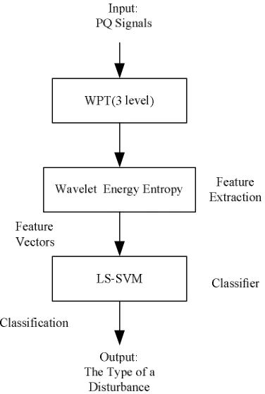
The types of PQ disturbances include the sag, inter-ruption, swell, harmonic, notch, oscillatory transient (Osc. transient) and impulsive transient (Imp. transient) (see Figure 1) [10]. In this paper, the combined tech-nique of wavelet packet transform (WPT) and least square support vector machines (LS-SVM) for PQ dis-turbances recognition is presented. Decision making is performed in two stages: feature extraction and LS-SVM as a classifier. Figure 2 shows the block diagram of the classification system. The details of each stage are de-scribed in the next sections. High accuracies were achieved by using the LS-SVM trained on the wavelet packet log-energy entropy of different nodes.

The rest of this paper is organized as follows. In Sec-tion 2, the feature extracSec-tion by WPT is explained. In Section 3, brief review of the LS-SVM with the mini-mum output coding (MOC) technique is presented.

Figure 1. Power quality disturbance waveforms: (a) Normal signal; (b) Sag; (c) Interruption; (d) Swell; (e) Harmonic; (f) Notch; (g) Oscillatory transient; (h) Impulsive transient.

Figure 2. Block diagram of the classification system.

the studied PQ disturbance signals are presented. Finally, conclusions are given in Section 5.

2. Feature Extraction Using WPT

The purpose of the feature extraction process is to select and retain relevant information from original signals. The WPT was first applied to decompose the original PQ signals into frequency bands. One of the advantages of the WPT is that it is able to decompose signals at various resolutions, which allows accurate feature extraction fro- m non-stationary signals like PQ disturbances. The fea-tures of signals, such as wavelet packet energy entropy, were then extracted from these decomposed signals as feature vectors.

The wavelet transform decomposes a signal into a set of basic functions called wavelets. These basic functions are obtained by dilations, contractions and shifts of a unique function called wavelet prototype. Continuous wavelets are functions generated functions generated from one single function by dilations and translations of a unique admissible mother wavelet ψ(t):

) ( 1 ) (

,

a b t a t b a

−

= ψ

ψ (1)

where a,b∈ℜ,a ≠ 0 are the scale and translation parameters, respectively, and t is the time. The func-tion set (ψa,b(t)) is called wavelet family. It is common to employ both wavelet and scaling functions in the transform representation. In general, the scale and shift parameters of the discrete wavelet family are given by

=

a j

a0 and

j a kb

b= 0 0, where j and k are

inte-gers. The function family with discretized parameters becomes:

) (

)

( 0

2 / 0

, t a a jt kb j

k

j = − −

− _ψ

ψ (2)

where ψj,k(t)is called the discrete wavelet transform (DWT) basis.

DWT analyzes the signal at different frequency bands, with different resolutions by decomposing the signal into a coarse approximation and detail information. DWT em- ploys two sets of functions called scaling functions ϕ(t) and wavelet functions ψ(t), which associated with low- pass and high-pass filters, respectively. The original sig-nal x(t) can be decomposed to:

∑ ∑

∑

= +

= J

j

jk k

jk k

t k d t

k c t

x _{j j}

1

) ( ) ( )

( ) ( )

( ϕ ψ (3)

where j is the level number of the wavelet decomposi-tion, j =1,2,L,J with J the time of the wavelet de- composition. cj and dj are the approximation

not be fine enough to extract pertinent frequency infor-mation about the signal. The necessary frequency resolu-tion may be achieved by using WPT, an extension of the DWT. In the WPT, the wavelet detail at each level is, in addition to decomposition of only the wavelet approxi-mation in the regular wavelet analysis, further decom-posed in to its own approximation and detail components. By this process, some lower frequency contents leaked in the wavelet details at the previous level can be further sifted out at the current level and also the frequency res- olution for signal analysis increases. As a result, the WPT may provide better accuracy in both higher and lower frequency components of the signal.

Figure 3 shows the wavelet packet decomposition tree for three levels (J =3). For each level of decomposition the signal is filtered into approximate information of the signals (lower frequency component) and detail informa-tion (higher frequency component). If this procedure is repeated J times, a filter bank is created with J filters. To evaluate the importance of the wavelet packet com- ponents to a signal, the concept of entropy is often ap-plied in signal processing and there are various defini-tions of entropy in the literature. Among them, two rep-resentative ones are used in the present article, i.e. the energy entropy and the Shannon entropy. The wavelet packet energy entropy at a particular node n in the wave-let packet tree of a signal is a special case of p = 2 of the

p-norm entropy, defined as

) 1 (

, ≥

=

∑

Ent p

k k n

n (4)

where wcn,kdenotes the wavelet packet coefficients

cor-responding to node n at time k. It was demonstrated that the wavelet packet energy has more potential for use in signal classification as compared to the wavelet packet coefficients alone. The wavelet packet energy represents energy stored in a particular frequency band and is mainly used in this study to extract the dominant fre-quency components of the signal.

The Shannon energy entropy and relative Shannon en-ergy entropy are defined respectively as [11]

Figure 3. Wavelet packet decomposition tree.

∑

− =

k

k n k

n

n wc wc

Ents log( 2 )

. 2

. (5)

n nor n

n Ents Ents

REnts = / _ (6)

where Entsnor_n is the Shannon energy entropy of the

normal signal corresponding to node n.

In this paper, one of the commonly used entropy, log- energy entropy is also defined as

∑

= k

k n

n wc

Entl log( 2 )

. (7)

The relative log-energy entropy is proposed as

n nor n

n Entl Entl

REntl = / _ (8)

where Entlnor_n is the log-energy entropy of the normal

signal corresponding to node n.

3. LS-SVM

The second stage is the disturbances classification. Sup-port vector machine (SVM) can avoid the problems of over learning, dimension disaster and local minimum in the classical study method, and is applied in many classi-fication problems successfully [8,11]. According to the practice, [12] advanced by J. A. K. Suyken can overcome the disadvantage of slow training velocity in the large scale problem, as LS-SVM algorithm translates the qua- dratic optimization problem into that of solving linear equation set. Although a wide range of classifiers are available, we use LS-SVM in this paper.

We consider a training set of N data points

{

}

N

k =1,2,L, , where n k

x ∈ℜ is the input data, yk ∈ℜ

is the k−th output data, the SVM constructs a deci-sion function that is represented by:

b x w x

y_{( )} = T + ₍₉₎

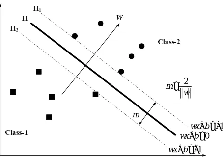
where the dimension of w is not specified. It means that it can be infinitely dimensional. The separating hyper-plane that creates the maximum distance between the plane and the nearest data is called as the optimal sepa-rating hyperplane as shown in Figure 4.

In LS-SVM for the function estimation the following optimization problem can be given

∑

=

+

= N

k k T

LS e b

w J w b e w w C e

1 2 2 1 2

1 ,

, ( , , )

min (10)

subject to the equality constraints

N k

e b x w

yk = T k + + k, =1,..., (11)

where ek are slack variables and C is a positive real

constant. One defines the Lagrangian

∑

= + + −

−

= N

k

k k k

T k

LS w x b e y

J e b w L

1

) (

) ; , ,

w m= 2

1

wx b+ = +

0

wx b+ =

1

wx b+ = − w

m

Figure 4. Optimal separating hyper plane.

with Lagrange multipliers αk. The conditions for

opti-mality are 1 1 0 0 0 0 0 0 k k N k k k N k k k k T

k k k

L _{w x}

w L b

L _e

e

L _{w x b e y}

α α α γ α = = ∂ = → = ∂  ∂ = → = ∂   ∂ = → = ∂  ∂  _{= → + + − =} ∂ 

∑

∑

for k =1,2,L,N. It can be written immediately as the solution to the following set of linear equations:

0 0 ₀

0 0 0

0 0 0 T w b γ −        _{    } −      ₌  ₋                 _{   }   I X I 1

I I I e

α Y

X 1 I

r

r

(14)

with X =[x1,...,xN], Y =[y1,...,yN], 1 =[1,...,1]

r

,e= 1

[ ,...,e eN] and α =[α1,...,αN]. The solution is finally

given by       =               + −

− _{α Y}

I X X 1 1 0 0 1 b T T γ r r (15)

with k

k kx

w=

∑

α are proportional now to the errors at the data points. So far we explained the linear case. SVM’s with polynomials, splines, radial basis function networks, or multilayer perceptrons as kernels are obtained after map-ping the input data into a higher dimensional space by

) (x_k

φ , where φ(⋅): ℜn → ℜnh. The number h n does not have to be specified because of the application of

Mercer’s condition, which means that

) ( ) ( ) ,

(xk xj xk T xj

K =φ φ (16) can be imposed for these kernels. Finally, the nonlinear function takes the form:

b x x K x y N k k k + =

∑

( α (17)

where the parameters αk, b follow from (15) after

replacing j T k x

x by K(xk,xj).

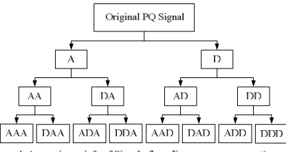
Multi-class classification was realized by the combi-nation of LS-SVM classifiers with the minimum output coding (MOC) technique. In the MOC technique, up to

m 2

log (where m is the number of classes) LS-SVM clas-sifiers were trained, and each of them aimed to separate a different combination of classes. There were eight classes (normal signal, sag, interruption, swell, harmonic, notch, oscillatory transient and impulsive transient) in this study, so three classifiers were necessary to differen-tiate them. The coding was defined by the codebook represented by a matrix, where the columns represent the different classes, and the rows indicate the results of the binary classifiers. The multi-class classifier output code for a pattern is a combination of targets of these three classifiers. In this study, the eight classes were encoded in the following codebook of minimum output coding:

T codebook C C C C C C C C           − − − − − − − − − − − − = 1 1 1 1 1 1 1 1 1 1 1 1 1 1 1 1 1 1 1 1 1 1 1 1 8 7 6 5 4 3 2 1

where C1,C2,C3,C4,C5,C6,C7,andC8 are normal signal, sag, interruption, swell, harmonic, notch, oscilla-tory transient and impulsive transient, respectively.

4. Simulation Analysis

To test classification results for PQ disturbances, the testing samples of these PQ disturbances have been gen-erated using algebraic equations [14]. The advantage of using algebraic equations for evaluation is the flexibility of adjusting signal noise contents as well as various waveform parameters such as the disturbance occurrence time, harmonic contents, sag depth, etc.

sys-tem disturbances.

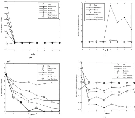
Using wavelet packet decomposition, each signal shown above was decomposed to level 3. The wavelet ‘Daub4’ was selected because it is more adequate for classifica-tion of PQ disturbances [13]. The wavelet packet energy entropy of different nodes of the decomposed signals were calculated, which could be used to identify the type of PQ disturbances. The performances of difference wave- let packet energy entropy for feature sets are shown in

Figure 5. From above Figure 5, we can conclude that relative log-energy entropy is more effective than tradi- tional relative Shannon energy entropy, which can am-plify the errors among the feature vectors. These features consist of 8-dimension feature space.

In this paper, we construct a LS-SVM by using radial basis function (RBF) as kernel function in LS-SVM pro-

posed above.

) 2 exp( ) , (

2 2

σ

j i j

i

x x x

x

K = − − ₍₁₈₎

where σ is the width of the kernel.

For training the SVMs with RBF kernel functions, one has to predetermine the σ values. The optimal or near optimal σ values can only be ascertained after trying out several, or even many values. Beside this, the choice of C parameter in the SVM is very critical in order to have a properly trained SVM. The SVM has to be trained for different C values until to have the best result. From the Figure 6, It is found that the near optimal val-ues are σ2 =1 _{and C} = _4.

node (a)

×105

node

(b)

×104

node (c)

node (d)

Each decomposed signal now has eight features (J

3

= ). The feature vectors of PQ disturbances are fed to the LS-SVM for classification. The LS-SVM topology used for classification is shown in Figure 7. We trained three different LS-SVMs (LS-SVM1, LS-SVM2, LSSV- M3) for seven different PQ disturbances (seven hundred samples of various PQ disturbances).The patterns to be distinguished from others are represented by +1 and the remaining patterns represented by -1 for both training and testing procedures.

The output of three different LS-SVMs constructs the code of the input PQ signals, which the type of a distur-bance or the normal signal will be identified. In the pre-sent work a standard feed-forward network with 8 input neurons, 12 hidden neurons, and 7 output neurons was compared to the LS-SVM implementation. Furthermore, our results indicate that solutions obtained by LS-SVM training seem to be more robust with a smaller standard

error compared to standard ANN training using the same features as inputs.

The other seven hundred PQ disturbances of various types have been generated for the testing. The classifica-tion results in a correct identificaclassifica-tion rate of 97.7% are shown in Table 1 using the proposed LS-SVM classifier. For comparison purposes, the total classification accura-cies on the same test sets and the CPU times of training of the two classifiers are presented in Table 2. It is found that the proposed LS-SVM classifier performed better than the standard ANN classifier.

To evaluate the performance of the kernel function, three LS-SVM classifiers were developed based on the linear kernel, the polynomial kernel, and the RBF kernel. The classification results with linear, polynomial and RBF kernel are shown in Table 3. The accuracy of clas-sification is high in RBF kernel in comparison with the polynomial and linear kernels.

Figure 6. Comparison of accuracy acquired with different

C and σ2 values for RBF kernels.

Table 1. Classification results using the proposed LS-SVM classifier.

Type of PQ disturbances

Number of disturbances

Number of disturbances

classified

Number of disturbances misclassified

Classification Accuracy

(%)

Sag 100 97 3 97

Interruption 100 97 3 97

Swell 100 99 1 99

Harmonic 100 98 2 98

Notch 100 99 1 99

Osc. transient 100 97 3 97

Imp. transient 100 96 4 96

Sum 700 684 16 97.7

Table 2. Comparison of the classification indices between the LS-SVM and ANN classifiers.

Classifier Training set samples

Testing set samples

Mean training time (s)

Mean testing ime (s)

Mean correct ratios (%)

LS-SVM 700 700 9.968 1.922 97.7

ANN 700 700 101.523 1.993 95.2

Table 3. Classification accuracies for the different kernels used.

Kernel used

Number of disturbances

in training

Number of disturbances

in testing

Number of disturbances misclassified

Classifica-tion accuracy (%)

Linear 700 700 27 96.1

Polynomial 700 700 20 97.1

RBF 700 700 16 97.7

[Yc1 Yc2 Yc3] Codebook' =

     

      

 

C8 C7 C6 C5 C4 C3 C2 C1 Decision

5. Conclusions

In this paper, an attempt has been made to extract effici- ent features of the PQ disturbances using WPT and to classify the disturbances using LS-SVM with the MOC technique. It is also found that relative wavelet packet log-energy entropy is considered as feature vectors, wh- ich are suitable for classification of PQ disturbances. For comparison different classifiers, the LS-SVM and ANN classifiers were implemented to deal with the same class- ification. The classification accuracies and the CPU tim- es of training showed that the LS-SVM classifier produc- es considerably better performance than that of the ANN classifier.

6. Acknowledgements

The authors would like to thank to the support of Wuhan Xinlian Science and Technology Ltd.

7. References

[1] S. Mallat, “A Wavelet Tour of Signal Processing,” Aca-demic Press, San Diego, California, 1998.

[2] S. Santoso, E. J .Powers and P. Hofman, “Power Quality Assessment via Wavelet Transform Analysis,” IEEE Transaction on Power Delivery, Vol. 11, No. 2, 1996, pp. 924-930.

[3] H. T. Yang and C. C. Liao, “A De-Noising Scheme for Enhancing Wavelet-Based Power Quality Monitoring System,” IEEE Transaction on Power Delivery, Vol. 16, No. 3, 2001, pp. 353-360.

[4] S. Santoso, E. J. Powers and W. M. Grady, “Power Qual-ity Disturbance Data Compression Using Wavelet Trans-form Methods,” IEEE Transaction on Power Delivery, Vol. 12, No. 3, 1997, pp. 1250-1257.

[5] A. K. Ghosh and D. L. Lubkeman, “The Classification of Power System Disturbance Waveforms Using a Neural

Network Approach,”IEEE Transaction on Power Deliv-ery, Vol. 10, No. 1, 1995, pp. 109-115.

[6] T. X. Zhu, S. K. Tso and K. L. Lo, “Wavelet-Based Fuzzy Reasoning Approach to Power Quality Distur-bance Recognition,”IEEE Transaction on Power Deliv-ery, Vol. 19, No. 4, 2004, pp. 1928-1935.

[7] M. B. I. Reaz, F. Choong, M. S. Sulaiman, F. Mohd- Yasin and M. Kamada, “Expert System for Power Qual-ity Disturbance Classifier,”IEEE Transaction on Power Delivery, Vol. 22, No. 3, 2007, pp. 1979-1988.

[8] P. Janik and T. Lobos, “Automated Classification of Power Quality Disturbances Using SVM and RBF Net-works,”IEEE Transaction on Power Delivery, Vol. 21, No. 3, 2006, pp. 1663-1669.

[9] J. Chung, E. J. Powers, W. M. Grady and S. C. Bhatt,

“Power Disturbance Classifier Using a Rule-Based Method and Wavelet Packet-Based Hidden Markov Model,”IEEE Transaction on Power Delivery, Vol. 17, No. 1, 2002, pp. 233-241.

[10] IEEE Recommended Practice for Monitoring Electric Power Quality, IEEE Standards Description: 1159-1995, 2009.

[11] G. S. Hu, F. F. Zhu and Z. Ren, “Power Quality Distur-bance Identification Using Wavelet Packet Energy En-tropy and Weighted Support Vector Machines,” Expert Systems with Applications, Vol. 35, No. 1-2, 2008, pp. 143-149.

[12] J. A. K. Suykens and J. Vandewalle, “Least Squares Sup-port Vector Machine Classifiers,”Neural Processing Let-ter, Vol. 9, No. 3, 1999, pp. 293-300.

[13] N. S. D. Brito, B. A. Souza and F. A. C. Pires, “ Daube-chies Wavelets in Quality of Electrical Power,” 8th In-ternational Conference on Harmonics and Quality of Power, Athens, 14-18 October 1998, pp. 511-515.