City, University of London Institutional Repository
Citation
:
Fairbank, M., Alonso, E. and Prokhorov, D. (2012). Simple and Fast Calculation
of the Second-Order Gradients for Globalized Dual Heuristic Dynamic Programming in
Neural Networks. IEEE Transactions on Neural Networks and Learning Systems, 23(10), pp.
1671-1676. doi: 10.1109/TNNLS.2012.2205268
This is the accepted version of the paper.
This version of the publication may differ from the final published
version.
Permanent repository link:
http://openaccess.city.ac.uk/5187/
Link to published version
:
http://dx.doi.org/10.1109/TNNLS.2012.2205268
Copyright and reuse:
City Research Online aims to make research
outputs of City, University of London available to a wider audience.
Copyright and Moral Rights remain with the author(s) and/or copyright
holders. URLs from City Research Online may be freely distributed and
linked to.
City Research Online:
http://openaccess.city.ac.uk/
[email protected]
Simple and Fast Calculation of the Second-Order
Gradients for Globalized Dual Heuristic Dynamic
Programming in Neural Networks
Michael Fairbank,
Student Member, IEEE
, Eduardo Alonso and Danil Prokhorov,
Senior Member, IEEE
(Published inIEEE Transactions on Neural Networks and Learning Systems, Vol.23, Issue 10, October 2012, pages 1671–1678. Copyright the authors and IEEE, http://ieeexplore.ieee.org.)
Abstract—We derive an algorithm to exactly calculate the mixed second order derivatives of a neural network’s output with respect to its input vector and weight vector. This is necessary for the Adaptive Dynamic Programming algorithms GDHP and Value-Gradient Learning. The algorithm calculates the inner product of this second order matrix with a given fixed vector in a time that is linear in the number of weights in the neural network. We use a “forward accumulation” of the derivative calculations which produces a much more elegant and easy-to-implement solution than has previously been published for this task. In doing so, the algorithm makes GDHP simple to implement and efficient, bridging the gap between the widely used DHP and GDHP Adaptive Dynamic Programming methods.
Index Terms—Neural Networks, Adaptive Dynamic Program-ming, Dual Heuristic ProgramProgram-ming, Value-Gradient Learning
I. INTRODUCTION
A
DAPTIVE Dynamic Programming (ADP) [1] is an im-portant methodology closely related to reinforcement learning, which is successfully used for solving control prob-lems in industry and research, including recent work by [2]–[5]. Dual Heuristic Dynamic Programming (DHP) and Globalized Dual Heuristic Dynamic Programming (GDHP) [6]–[8] are two important algorithms used in ADP.Out of these two algorithms, DHP has been used far more often than GDHP in successful applications. For example DHP has been used in control problems [7], [9], power grid control [10], [11], and many others applications [1]. One of the reasons for the comparatively low take-up of GDHP is that GDHP is more challenging to implement than DHP. The difficult step of implementation is to correctly and efficiently calculate the second order mixed partial derivatives of a neural network’s scalar outputy=y(~x, ~w)with respect to its input vector~xand weight vector w, i.e. the matrix~ ∂ ~∂w∂~2yx (where we define this second derivative notation such that this matrix has the element at(i, j)equal to∂ ~w∂j2∂~yxi). This matrix is related to, but slightly
different to, the usual Hessian matrix, ∂ ~∂w∂ ~2yw, described in the neural network literature (e.g. sec. 4.10 of [12]).
The GDHP algorithm, which we describe in detail in section IV, only requires this second derivative matrix ∂ ~∂w∂~2yx as an inner product ∂ ~∂w∂~2yx~k, where ~k is a column vector constant
M. Fairbank and E. Alonso are with the Department of Computing, School of Informatics, City University London, London, UK
D. Prokhorov is with Toyota Research Institute NA, Ann Arbor, Michigan Manuscript received August 2011
of dimension dim(~x). To form this inner product by matrix-vector multiplication would take time O(dim(w~) dim(~x)2).
In this paper, we provide a very clear and straightforward algorithm to calculate this inner product directly and exactly in an asymptotically faster time of O(dim(w~)).
Existing literature does briefly outline an equally efficient method to calculate the required inner product, but this outline is only in the form of schematic diagrams [7], or a high level description of generic backpropagation [13], [14]. Sim-ple pseudocode applicable for a generic feed-forward neural network is not available there.
All of these existing descriptions calculate the required second derivatives by applying the mathematical technique of backpropagation twice to the neural network’s feed-forward equations [15]. Using the terminology of “automatic differ-entiation” [16], [17], this is called a reverse accumulationof the derivatives. But it is not a trivial task to create a correct implementation of this for the given error function. In fact this difficulty is thought to be one of the reasons that the equations for the required second order derivatives have not been published before for a generic neural network.
Our method is to do aforward accumulationof the deriva-tives. This is much easier to derive and implement, and equally efficient. Our method follows the technique and terminology of [18], which is used to calculate an inner product of the Hessian matrix of a neural network in a fast and exact manner, without explicitly finding the full Hessian matrix itself.
The difference in simplicity in derivation between the for-wards and backfor-wards accumulation methods is very signif-icant, as is illustrated by the way the two techniques were used to find fast products with the Hessian matrix, in the neural network literature. Here, the backward accumulation is described by [19], and the derivation takes several pages (dense with lemmas and equations). The forward accumulation is described by [18], and the derivation takes just one page to define a differential operator (“R”), which then is used to produce the five lines of the algorithm instantly. Despite the technically demanding accomplishment of [19], it is the vastly simpler technique of [18] that receives nearly all of the citations in the literature.
pseudocode for the resulting algorithm, we intend to solve the problem of GDHP being more difficult to implement than DHP.
Besides being useful for GDHP, the quantity ~kT ∂2y ∂ ~w∂~x is
also useful in the general circumstance of trying to adjust the weights of a neural network so as to force the gradient ∂y∂~x to equal a given target value at a given ~x. To achieve this, we would do gradient descent on an error functionE= 12|∂y∂~x−~t|2,
where~tis the “target” gradient. In this case we would choose the constant vector~k by
~k= ∂E ∂(∂y/∂~x)=
∂y
∂~x−~t (1)
We give an example of an application like this in section III-B. An extension algorithm to GDHP is Value-Gradient Learn-ing [20]–[22], and this can require a further inner product, ~
kT ∂2y
∂~x∂~x, which is also produced by the algorithm.
In the rest of this paper, in section II we define the neural network and gradient finding algorithms. In section III we give experimental results for a neural network problem, and in section IV we define ADP and show how our algorithm can be used with GDHP. Finally, in section V we give conclusions.
II. THEALGORITHMS
In this section we describe the algorithm to find the second order gradients that this paper requires. We define a very general feed-forward neural network architecture in section II-A, and derive the second derivatives for it in section II-B. We describe how the method can be extended to find the full second derivative matrices in section II-C.
The way we derive the second-derivative matrices for this neural network is a general technique that could be applied to any existing feed-forward network structure (or even a recurrent neural network that has been unrolled using back-propagation through time), and we describe how we would validate any algorithm’s correctness in section III-A.
A. Feed-forward Neural Network Architecture and Backprop-agation
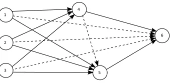
Lines 2 to 8 of Algorithm 1 implement a general neural network y(~x, ~w), which has a single input layer, and is fully connected with all shortcut connections. The algorithm takes an input vector ~xand weight vectorw, and, for the purposes~ of this paper, produces a scalar output y. Pruned or layered network architectures are possible by fixing specific weights to zero. Fig. 1 illustrates an example network attainable by the algorithm.
In the algorithm, superscripts on variable names indicate the node number, for j = 0, . . . , n, where nis the final node in the network. The variablesajrepresent the firing activations of
nodej, and the final node’s activation,an, gives the network’s
output,y. Node 0 is a dedicated “bias” node, with a fixed value of a0 = 1. ~x = x1 x2 . . . xm is the external input vector to the whole network, with dimension m = dim(~x). We use the notationwk,j to indicate the weight withinw~ that connects node k to node j. sj, δaj and δsj are workspace scalars for each node.
1 2
3 5
[image:3.612.354.523.51.134.2]6
Fig. 1. An example neural network architecture obtainable by Algorithm 1, with three input nodes and one output node. When all graph edges are included, we have a fully connected feed-forward neural network, with all shortcut connections. If the dotted edges are removed (for example by clamping those weights to zero) then a more traditional layered network is obtained, containing a single hidden layer of two nodes. For the purpose of this paper we always require a single output node, which in this example is node 6.
Algorithm 1 Feed-forward Dynamics of a neural network followed by First Order Error Backpropagation to Calculate
∂y ∂~x
1: {Feed-forward input vector~xthrough network...}
2: a0←1 {Bias node}
3: ∀j: 1≤j≤dim(~x), aj ←xj {Input vector,~x} 4: forj= dim(~x) + 1tondo
5: sj ←Pj−1
m=0w m,jam
6: aj ←g(sj)
7: end for
8: y←an {Network Output} 9: {Backpropagation loop...} 10: forj=nto1 step−1 do
11: δaj ←
(
1 ifj=n
Pn
m=j+1(w
j,m)(δsm) otherwise
12: δsj←(δaj)g0(sj)
13: ∀m: 0≤m < j, ∂w∂ym,j ←(δs
j)am
14: end for
15: ∀j: 1≤j≤dim(~x), ∂x∂yj ←δa
j {Output Vector}
g(x) : < → < is the “activation function”, which is often taken to beg(x) = tanh(x), or the logistic function,g(x) =
1
1+e−x.g0(x)andg00(x)are its first and second derivatives.
Lines 10 to 15 of Algorithm 1 do a backpropagation calculation, which calculates the gradients ∂y∂~x and ∂ ~∂yw. This is the standard backpropagation algorithm for neural networks [15], [23] but modified, following [24], so that the “error function” used is actually the network output y, and also so that the backward pass continues until it has fully generated the quantity ∂~∂yx, as required.
B. Finding Second Derivatives using theROperator
Hence we defineR(.)as the differential operator
R=X
i
ki ∂
∂xi (2)
whereki is theith component of~k.
Using this operator, the two second derivatives that we seek can now be written as R(∂ ~∂yw)andR(∂y∂~x), respectively.
Also, applying this R operator to~xgives:
R(~x) =X i
ki ∂ ∂xi~x
=~k (3)
As detailed by [18],Robeys the usual rules for a differential operator, i.e. it obeys the product rule, the chain rule, the sum rule for derivatives, and differentiating a constant gives zero. For example, the weight vectorw~ is a constant with respect to theRoperator, thusR(w~) =~0. Using these rules, and (3), we apply theRoperator to each side of each line of Algorithm 1, to obtain each line of Algorithm 2, respectively. We emphasise that applying the R operator to each line of the algorithm, while obeying the correct rules for differential operators, is calculating the exact derivatives that we are seeking. See section 3 of [18] for further explanation of the exactness of the R method.
Hence Algorithm 2 exactly calculates the quantitiesR(∂ ~∂yw)
and R(∂y∂~x), which are the two second-derivative inner-products that we seek.
Algorithm 2 Calculation of the Second Order Derivatives
Require: sj, aj,δsj andδaj values calculated according to
Alg. 1 for all nodes j, and vector ~k calculated by an appropriate equation (e.g. (1))
1: {Forward pass...} 2: R(a0)←0
3: ∀j: 1≤j≤dim(~x), R(aj)←kj
4: forj= dim(~x) + 1tondo
5: R(sj)←Pj−1
m=0w
m,jR(am)
6: R(aj)←g0(sj)R(sj)
7: end for
8: {Backward pass...} 9: forj=nto1step −1 do
10: R(δaj)←
(
0 ifj=n
Pn
m=j+1(w
j,m)R(δsm) otherwise
11: R(δsj)←R(δaj)g0(sj) + (δaj)g00(sj)R(sj)
12: ∀m : 0 ≤ m < j, R(∂w∂ym,j) ← R(δsj)(am) +
(δsj)R(am){Output vector 1:~kT ∂2y ∂ ~w∂~x}
13: end for
14: ∀j: 1≤j≤dim(~x), R(∂x∂yj)←R(δaj) {Output vector
2:~kT ∂2y ∂~x∂~x}
When implementing the algorithm, R(aj), R(sj), R(δaj)
andR(δsj)are workspace scalars for each nodej.
C. Generating the Full Second Derivative Matrices
The above algorithm generates the inner products of two second order derivative matrices with a constant vector. If
instead of this inner product, the full second order derivative matrices are required, then these can be constructed one column at a time. Execution of the above algorithms with ~k equal to thejth Euclidean standard basis vector of dimension
dim(~x), will calculate thejth column of each matrix. Thus ac-cumulating the full second order matrices, column by column, would take O(dim(w~) dim(~x)) time.
An alternative algorithm to find the full matrix ∂ ~∂w∂~2yx is given for a neural network with just one hidden layer by equations 14 and 15 of [7], and for a general network by appendix A.4 of [25]. These also have asymptotic timings of O(dim(w~) dim(~x)).
III. EXPERIMENTALRESULTS
We describe how we validated the correctness of the algo-rithm in section III-A, and describe a simple experiment that shows how a neural network can be forced to learn a target quantity ∂y∂~x in section III-B.
A. Numerical Verification of the Algorithm
To validate the algorithm was calculating the correct sec-ond order gradients, we used numerical differentiation. This method provides a flexible and powerful check of the correct-ness of the program. Since theR method could be applied to other neural network architectures, it would be advisable to verify any other implementation in a similar manner.
To do the numerical confirmation, we first verified the formation of ∂y∂~x and ∂ ~∂yw taking place in lines 10 to 15 of Algorithm 1, by differentiatingy numerically with respect to both~xandw, respectively. For example, to verify the first of~ these, we used a central-differences numerical derivative:
∂y ∂xi =
y(~x+~ei, ~w)−y(~x−~ei, ~w)
2 +O(
2)
whereis a small positive constant, and~eiis theith Euclidean
standard basis vector.
We next checked the second derivatives found by Algorithm 2 against a first order numerical differentiation of the (already tested) first order analytical derivatives found by Algorithm 1. For example,
~kT ∂
∂~x
∂y
∂ ~w
= ∂y ∂ ~w
(~x+~k, ~w)−
∂y ∂ ~w
(~x−~k, ~w)
2 +O(
2) (4)
TRAININGDATA FOREXPERIMENT1.
xp(Network input) sp(Target fory) tp(Target for ∂y∂~x)
0.0 0 20
0.25 0 -20
0.5 0 20
0.75 0 -20
1.0 0 20
B. Wave Learning Experiment
In this experiment we provide an example of how the algorithms of this paper can be used to adjust the weights of a neural network so as to force the gradient ∂y∂~x to equal a given target value at a given~x.
The objective here is to make a neural network with one input and one output learn the training data given in table I. In this training data, each row of the table is a different “pattern”, p. Each pattern consists of an input value for the neural network (xp), and target output value (sp) and a target
for the gradient ∂y∂~x (tp). This experiment is aiming to make
a neural network learn two complete periods of a sine wave from just 5 training patterns positioned along the x-axis.
Learning took place by minimising the error function given in (5).
E=1 2
5
X
p=1
η1(y(xp, w)−sp) 2
+η2
∂y ∂~x
(xp,w)
−tp
!2
(5)
η1 and η2 are real constants to weight the relative
signifi-cance of the two terms in this equation. The first term is an ordinary sum-of-squares error for making the network output y(x, ~w)match the target output for each pattern. The gradient of this part of the error function (with respect tow) would be~ found by ordinary backpropagation. The second term ofEis a sum-of-squares error term for making the gradient ∂~∂yx match the target gradient tp for each pattern p. Hence this second
term would form the vector~kdescribed in (1) by
~k= ∂y ∂~x
(x
p,w)
−tp
for each patternp, and then the required gradient for learning can be found by Algorithm 2.
The neural network used was a multi-layer perceptron, with two hidden layers of 8 nodes each, and all shortcut connections present between all pairs of non-adjacent layers. The activation function used for all nodes was g(x) = 1/(1 +e−x), except for the output node which used g(x) = x. Training used gradient descent on (5), with η1=η2= 1, i.e. with the same
[image:5.612.67.279.78.138.2] [image:5.612.319.562.243.357.2]significance attached to each component of the error function. Initial network weights were randomised uniformly from [-0.1,0.1].
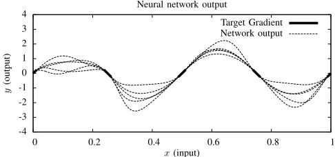
When training was accelerated through conjugate gradients, with a full line search, learning produced a 100% convergence rate over 100 trials, where convergence was defined asEgoing below10−5within 20000 iterations. The output of five typical neural networks trained in this way are shown in Fig. 2.
The results show that the problem has been solved correctly, and that it has been possible to make a neural network learn specified target gradients ∂y∂~x at given values of ~x. However when experimental parameters were changed, we observed that the success rate could drop significantly. For example if RPROP was used, and the activation functions used were swapped to g(x) = tanh(x), then the success rate dropped from 100% to 65%. It seems that it is harder to train a neural network to learn target gradients, ∂y∂~x, than target values. By analogy we can imagine that in trying to make the flexible curves of Fig. 2 bend into the shape of a sine wave, it is harder to do so by just twisting the curve at certain points along the x-axis than it is by stretching the curve to pass through given target points.
-4 -3 -2 -1 0 1 2 3 4
0 0.2 0.4 0.6 0.8 1
y
(output)
x(input) Neural network output
Target Gradient Network output
Fig. 2. Outputs from a sample of five neural networks created in the experiment of section III-B. Each dotted curve shows the output from a neural network produced in a different trial. The solid thick lines on the x-axis are designed to give a visual indication of the training point and target gradient. The objective of training is to make the dotted lines run parallel and through the thick lines, which has been achieved well in all of the five network outputs in this figure.
IV. ADAPTIVEDYNAMICPROGRAMMING
In this section, we describe adaptive dynamic programming, and in sections IV-A and IV-B we define the algorithms GDHP and DHP, showing how the methods of this paper can be applied to GDHP. We describe a simple GDHP experiment in section IV-C. However we point out that since the methods of our paper calculate ~kT ∂2Je
∂ ~w∂~x exactly, the empirical results
in using GDHP with it will be identical to any other exact method.
In Adaptive Dynamic Programming, an agent moves in an environment such that at timetit has state vector~xt. At each
time the agent chooses an action~utwhich takes it to the next
state according to the environment’s model function ~xt+1 =
f(~xt, ~ut), thus the agent passes through a trajectory of states (~x0, ~x1, ~x2, . . .). On transitioning from each state ~xt to the
next, the agent receives an immediate scalar costUtfrom the
environment according to the function Ut=U(~xt, ~ut).1
The ADP problem is for the agent to learn how to choose actions so as to minimise the expectation of the total long term cost received,J(~x0) =hP
tγ tU
ti, from any given start state
~
x0, whereγ∈[0,1]is a constantdiscount factorthat specifies
1Throughout this section, subscripts indicate the time step of a trajectory,
the importance of long term costs over short term ones.2 Specifically, the problem is to find anaction networkA(~x, ~z), where ~z is the parameter vector of a function approximator, that calculates which action~u=A(~x, ~z)to take for any given state ~x, such that this total long term cost is minimised.
To aid training the action network, ADP algorithms make an intermediate goal to first learn a scalar “critic” function
e
J(~x, ~w)over the state space. This function is the scalar output of a function approximator (e.g. a neural network with one output node) with parameter vector w, and the objective of a~ critic-learning algorithm is for the critic function to be trained to equal the cost-to-go function J(~x) over all of the state space. The function J is also known as the value function from dynamic programming [26].
A. The GDHP Algorithm
The GDHP algorithm is a critic learning algorithm that attempts to learn the functionJe(~x, ~w)by making its gradient
∂Je
∂~x explicitly match the gradient of the cost-to-go function, ∂J
∂~x. For each time step t of a trajectory (~x0, ~x1, ~x2, . . .), the
GDHP algorithm is defined to be the following critic weight update:
∆w~i=η1
∂Je
∂ ~wi !
t
(Ut+γJet+1−Jet) +η2 X
j
∂2Je
∂ ~wi∂~xj ! t ~ Et j (6)
whereη1andη2are small positive learning rates
correspond-ing to a learncorrespond-ing rate for the values of J, and a learning rate for the gradients ∂J∂~x, respectively; whereJe(~x, ~w)is the critic
function; whereE~t∈Rdim(~x) is a vector defined to be
~ Et=
DU D~x
t
+γX
j Dfj D~x t
∂Je
∂~xj !
t+1
− ∂Je
∂~x
!
t
(7)
and D~Dx is shorthand for
D D~x ≡
∂ ∂~x+
X
j
∂Aj
∂~x ∂
∂~uj ; (8)
where all of these derivatives are assumed to exist;j is a free variable to indicate a vector component, so that for exampleAj
refers to thejth component of the output of the action network; and where the subscripted t indicates that a function is to be evaluated at the state ~xt (and action ~ut, where relevant),
so that, for example Jet+1 ≡ Je(~xt+1, ~w) and
Df
D~x
t is the
derivative Df(~D~x,~xu) evaluated at(~xt, ~ut).
Equations (6), (7) and (8) define the GDHP algorithm. See [6], [7] for further details.
In GDHP, the function Je(~x, ~w) would be the output of a
neural network with one single output node, i.e. the function
e
J takes the role ofyin the descriptions of the rest of this paper. Consequently the appearance of ∂2Je
∂ ~w∂~x in (6) is a requirement
for a calculation of the second order gradients described by this paper. To use our method for GDHP, we would run Algorithm 2 with~k=E~t according to (7).
2If the problem is such that the trajectory is not guaranteed to terminate,
then to prevent an infinite total cost,γshould also satisfyγ <1.
The other gradients of Jeappearing in (6) and (7), i.e. ∂∂ ~Jwe
and ∂Je
∂~x, can be found by Algorithm 1 (in lines 13 and 15,
respectively). The derivatives of f(~x, ~u) andU(~x, ~u) should be available from the environment, since in the GDHP method we assume these functions are known and differentiable.
Once the critic function has been learned (or during con-current learning of both the critic and the action network), the weight vector for the action networkA(~x, ~z)can be updated by the following weight update:
∆~zi=−βX
j
∂Aj ∂~zi
t
∂U ∂~uj
t
+γX
k
∂fk ∂~uj
t
∂Je
∂~xk !
t+1 !
(9)
where β is a separate learning rate for the action network. The multiplications by ∂A∂~z and ∂A∂~x, in equations (9) and (8) respectively, can be done quickly and exactly by ordinary backpropagation.
B. DHP algorithm and its relationship to GDHP
The DHP algorithm is almost identical to GDHP, but the scalar critic Je(~x, ~w) is removed, and instead a new neural
network of input and output dimensiondim(~x)is used, which we call the vector critic,~λ(~x, ~w). The purpose of this vector critic is to simulatethe gradient ∂Je
∂~x. Hence the DHP weight
update is similar to (6), but all occurrences of ∂Je
∂~x are replaced
by~λ, and the constant η1 must be fixed at zero (sinceJet is
not defined). Hence the DHP critic weight update is:
∆w~i=η2 X
j
∂~λj ∂ ~wi
! t ~ Et j (10)
where both instances of∂Je
∂~x in (7) are replaced by~λ. A similar
replacement is done for the DHP actor weight update (9). The DHP weight update (10) is a much simpler weight update than the GDHP one of (6), since there is no requirement for second order differentiation. This is why DHP has so far always been simpler to program than GDHP. Another advantage of DHP over GDHP is that training a neural network to learn target values can be easier than training one to learn target gradients (as discussed at the end of section III-B). However GDHP is possibly advantageous over DHP in that its critic function is a true scalar field, just like its intended target, the cost-to-go functionJ(~x); although it remains to be seen whether GDHP is advantageous in practice.
C. GDHP Experiment
We now provide an extremely simple quadratic optimisation experiment using GDHP.
We define an environment with~x≡x∈ <and~u≡u∈ <, and model and cost functions:
f(x, t, u) =
(
x+u ift= 0
x ift= 1
U(x, t, u) =
(
0 if t= 0 (x)2 if t= 1
final cost being received on transitioning from to ). In these model function definitions, action u1 has no effect,
so the whole trajectory is parametrised by justx0andu0. The
total cost for this trajectory is(x0+u0)2, so the optimal action
to choose isu0=−x0.
The action network A(~x, ~z)was a layered neural network with two inputs, one output and one hidden layer of 4 nodes, shortcut connections from the input layer to the output layer, and with activation function g(x) = tanh(x) on all nodes. The weights ~z were initially randomly chosen from [-0.1, 0.1] uniformly. The critic network Je(~x, ~w) was identically
dimensioned to the action network, with a weight vector w~ randomised initially in the same way. The activation function used for the critic was g(x) = tanh(x) on all nodes except for the output node, which used g(x) =x. The input vector to each neural network was (x, t), since in this problem the optimal cost-to-go function depends on both of these inputs.
We applied the GDHP and action network learning equa-tions (6) and (9) concurrently, using learning rate constants η1 = 0, η2 = 0.1 andβ = 0.1, and discount factor γ = 1.
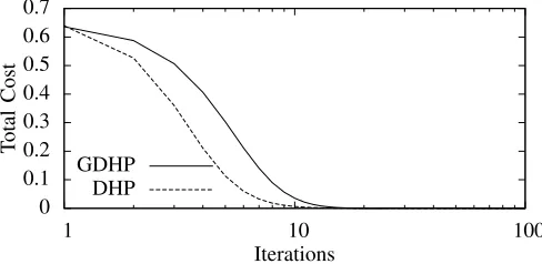
Each iteration of training consisted of the application of these two weight updates accumulated over all non-terminal time steps of the trajectory, t ∈ {0,1}. Each trajectory started fromx= 0.8. Experimental results, for both GDHP and DHP, averaged over 10 trials are shown in Fig. 3. The graph shows that both algorithms can solve this problem in similar time. DHP is slightly faster, but with this being such a simple test problem the slight difference between the two algorithms is not significant.
0 0.1 0.2 0.3 0.4 0.5 0.6 0.7
1 10 100
T
otal
Cost
Iterations GDHP
[image:7.612.45.289.421.540.2]DHP
Fig. 3. Results for GDHP and DHP in solving the problem described in section IV-C. Both GDHP and DHP manage to reduce the total cost to almost zero within 100 iterations.
V. CONCLUSIONS
We have presented a very clear and straightforward algo-rithm to find the product~kT ∂2y
∂ ~w∂~x exactly in time O(dim(w~)).
We have found that using a forward accumulation of the derivatives leads to an extremely easy way to derive the algorithm, in comparison to a backward accumulation that GDHP practitioners have relied upon until now.
We have made the appropriate modifications to the R method of [18] enabling us to derive the algorithm quickly. We have provided an empirical demonstration of the problem of learning target gradients in a neural network, and we have placed emphasis on the applicability to GDHP, giving an
example. It is the intention of this paper that implementing GDHP should be as straightforward as implementing DHP, while having an equivalent (O(dim(w~))) running time too.
REFERENCES
[1] F.-Y. Wang, H. Zhang, and D. Liu, “Adaptive dynamic programming: An introduction,” IEEE Computational Intelligence Magazine, vol. 4, no. 2, pp. 39–47, 2009.
[2] F.-Y. Wang, N. Jin, D. Liu, and Q. Wei, “Adaptive dynamic programming for finite-horizon optimal control of discrete-time nonlinear systems with
-error bound,”IEEE Transactions on Neural Networks, vol. 22, no. 1, pp. 24–36, 2011.
[3] J. Fu, H. He, and X. Zhou, “Adaptive learning and control for mimo system based on adaptive dynamic programming,”IEEE Transactions on Neural Networks, vol. 22, no. 7, pp. 1133–1148, 2011.
[4] K. M. Iftekharuddin, “Transformation invariant on-line target recogni-tion,”IEEE Transactions on Neural Networks, vol. 22, no. 6, pp. 906– 918, 2011.
[5] Y. Jiang and Z.-P. Jiang, “Approximate dynamic programming for opti-mal stationary control with control-dependent noise,”IEEE Transactions on Neural Networks, vol. 22, no. 12, pp. 2392 –2398, 2011.
[6] P. J. Werbos, “Approximating dynamic programming for real-time control and neural modeling.” inHandbook of Intelligent Control, White and Sofge, Eds. New York: Van Nostrand Reinhold, 1992, ch. 13, pp. 493–525.
[7] D. Prokhorov and D. Wunsch, “Adaptive critic designs,”IEEE Transac-tions on Neural Networks, vol. 8, no. 5, pp. 997–1007, 1997. [8] S. Ferrari and R. F. Stengel, “Model-based adaptive critic designs,” in
Handbook of learning and approximate dynamic programming, J. Si, A. Barto, W. Powell, and D. Wunsch, Eds. New York: Wiley-IEEE Press, 2004, pp. 65–96.
[9] G. G. Lendaris and C. Paintz, “Training strategies for critic and action neural networks in dual heuristic programming method,” inProceedings of International Conference on Neural Networks, Houston, 1997. [10] G. K. Venayagamoorthy and D. C. Wunsch, “Dual heuristic
program-ming excitation neurocontrol for generators in a multimachine power system,”IEEE Transactions on Industry Applications, vol. 39, pp. 382– 394, 2003.
[11] G. K. Venayagamoorthy, R. G. Harley, and D. C. Wunsch, “Comparison of heuristic dynamic programming and dual heuristic programming adaptive critics for neurocontrol of a turbogenerator,”IEEE Transactions on Neural Networks, vol. 13, no. 3, pp. 764–773, 2002.
[12] C. M. Bishop, Neural Networks for Pattern Recognition. Oxford University Press, 1995.
[13] P. J. Werbos, “Neural networks, system identification, and control in the chemical process industries.” inHandbook of Intelligent Control, White and Sofge, Eds. New York: Van Nostrand Reinhold, 1992, ch. 10, pp. 283–356.
[14] ——, “Building and understanding adaptive systems: a statisti-cal/numerical approach to factory automation and brain research,”IEEE Trans. Syst. Man Cybern., vol. 17, no. 1, pp. 7–20, Jan. 1987. [15] ——, “Beyond regression: New tools for prediction and analysis in the
behavioral sciences,” Ph.D. dissertation, Harvard University, 1974. [16] L. B. Rall, “Automatic differentiation: Techniques and applications,”
Lecture Notes in Computer Science, vol. 120, 1981.
[17] P. J. Werbos, “Backwards differentiation in AD and neural nets: Past links and new opportunities,” inAutomatic Differentiation: Applications, Theory, and Implementations, ser. Lecture Notes in Computational Science and Engineering, H. M. B¨ucker, G. Corliss, P. Hovland, U. Nau-mann, and B. Norris, Eds. Springer, 2005, pp. 15–34.
[18] B. A. Pearlmutter, “Fast exact multiplication by the Hessian,” Neural Computation, vol. 6, no. 1, pp. 147–160, 1994.
[19] M. Møller, “Exact calculation of the product of the hessian matrix of feed-forward network error functions and a vector in o(n) time,” Aarhus University, Tech. Rep. DAIMI PB-432, 1993.
[20] M. Fairbank and E. Alonso, “Value-gradient learning,” inProceedings of the IEEE International Joint Conference on Neural Networks 2012 (IJCNN’12). IEEE Press, June 2012, pp. 3062–3069.
[23] D. Rumelhart, G. Hinton, and R. Williams, “Learning representations by back-propagating errors,”Nature, vol. 6088, pp. 533–536, 1986. [24] J. Kindermann and A. Linden, “Inversion of neural networks by gradient
descent,”Parallel Computing, vol. 14, pp. 277–286, 1990.
[25] R. Coulom, “Reinforcement learning using neural networks, with appli-cations to motor control,” Ph.D. dissertation, Institut National Polytech-nique de Grenoble, 2002.