Discrete-time volatility forecasting with persistent leverage effect and the link with continuous-time volatility modeling

City, University of London Institutional Repository

Citation

:

This is the accepted version of the paper.

This version of the publication may differ from the final published

version.

Permanent repository link: http://openaccess.city.ac.uk/4434/

Link to published version

:

Copyright and reuse:

City Research Online aims to make research

outputs of City, University of London available to a wider audience.

Copyright and Moral Rights remain with the author(s) and/or copyright

holders. URLs from City Research Online may be freely distributed and

linked to.

City Research Online: http://openaccess.city.ac.uk/ [email protected]

Discrete-time volatility forecasting with persistent leverage effect

and the link with continuous-time volatility modeling

Fulvio Corsi† Roberto Ren`o‡

January 10, 2012

Abstract

We first propose a reduced form model in discrete time for S&P500 volatility showing that the forecasting performance can be significantly improved by introducing a persistent leverage effect with a long-range dependence similar to that of volatility itself. We also find a strongly significant positive impact of lagged jumps on volatility, which however is absorbed more quickly. We then estimatecontinuous-timestochastic volatility models which are able to reproduce the statistical features captured by the discrete-time model. We show that a single-factor model driven by a fractional Brownian motion is unable to reproduce the volatility dynamics observed in the data, while a multi-factor Markovian model fully replicates the persistence of both volatility and leverage effect. The impact of jumps can be associated with a common jump component in price and volatility.

JEL classification: C13; C22; C51; C53

Keywords: Volatility Forecasting; Leverage Effect; Jumps; Fractional Brownian Motion; Multifactor Models.

∗_{This paper supersedes the previously circulating versionsVolatility determinants: heterogeneity, leverage and}

jumps and HAR volatility modelling with heterogenous leverage and jumps. The paper is complemented by a Web Appendix downloadable from our web pages and containining supplementary material. The daily variables used in this paper are available from the authors upon request. We would like to acknowledge Davide Pirino for research assistence, Federico Bandi, Tim Bollerslev, Alvaro Cartea, Giampiero Gallo, Roel Oomen, Eduardo Rossi, Paolo Santucci de Magistris and Fabio Trojani for useful suggestions, and the partecipants at the SITE Summer Segment in Stanford, June 2009 and at seminars in Madrid, Universidad Carlos III and Tokio, Bank of Japan. Universit`a della Svizzera Italiana and Carey Business School at Johns Hopkins University are kindly acknowledged for support. All errors and omissions are our own.

†_{University of St. Gallen and Swiss Finance Institute, E-mail: [email protected]}

1

Introduction

The relevance of financial market volatility led to a very large literature trying to take into

account its most salient dynamic features: clustering, slowly decaying auto-correlation,

asym-metric responses. The advent of high-frequency data, allowing for specification and estimation

of models for realized volatility, elicited a considerable advancement in this field. However, a

considerable gap still exists in the literature between models devised for volatility forecasting,

which are commonly specified in discrete time, and volatility modeling in continuous time which

is used, among other things, for option pricing. This is particularly annoying for leverage effect,

whose interpretation is completely different in discrete time, where it is typically interpreted as

a negative correlation between lagged negative returns and volatility, and in continuous time,

where the negative correlation between price and volatility shocks is contemporaneous.

This paper contributes to this literature in two directions and aims at filling this apparent gap.

In the first part of the paper, we propose a new reduced-form model indiscrete time, the

LHAR-CJ model, which is able to provide a remarkable forecasting performance for volatility over a

time horizon which ranges from one day to one month, along with a positive and significant

risk-return trade-off. Our specification is extremely simple to implement and it is based on the

incorporation of three effects. The first is the well know volatility persistence, which is modeled

with the HAR specification of Corsi (2009). However, we do not restrict to lagged volatilities

(at daily, weekly and monthly frequency) as possible sources of future volatility, but we also

add jumps (as in Andersen et al., 2007) and, as a novel contribution of this paper, negative

returns over the past day, week and month, thus imposing a common heterogeneous structure

to the explanatory variables.

The empirical findings in the first part of the paper are also relevant because of the

impor-tant implications they bear on the set of continuous-time models consistent with the empirical

features of financial data. In the second part of the paper, we then estimate continuous-time

thus reproducing the very same features captured by the discrete-time model. In particular, we

show that a single-factor model is unable to reproduce the type of integrated volatility

persis-tence which is displayed by the data, even when allowing shocks to be driven by a fractional

Brownian motion (Comte and Renault, 1998), that is by a genuine long-memory component.

This induces us to investigate multi-factor specifications. We find that a Markovian two-factor

model is able not only to replicate the persistence of integrated volatility, but also the

persis-tence in the leverage effect by correlating more than one volatility factor with the price shocks.

The analyzed multi-factor models do not need long-memory shocks to achieve their goal. While

not ruling out the possible presence of long memory in volatility, this shows that the

autocorre-lation function of realized volatility is not necessarily a signature of genuine long memory in the

data generating process, and corroborates the framework according to which market volatility

is generated by a superposition of different frequencies, as suggested in Corsi (2009) and Muller

et al. (1997).

In the literature, it is well known that volatility tends to increase more after a negative shock

than after a positive shock of the same magnitude see e.g. Christie (1982); Campbell and

Hentschel (1992); Glosten et al. (1989) and more recently Bollerslev et al. (2006), Bollerslev

et al. (2009) and Martens et al. (2009). We extend the heterogeneous structure to the

stan-dard leverage effect by including lagged negative returns at different frequencies as explanatory

variables to forecast volatility. This idea traces back to Corsi (2005) and can also be found in

concurrent work of Scharth and Medeiros (2009) and Allen and Scharth (2009) as well as in

Fernandes et al. (2009) to forecast implied volatility. However, with this paper we are able to

provide a novel and clear evidence on the fact that the impact of negative returns on future

volatility of S&P500 is also highly persistent and extends for a period of at least one month,

thus displaying a long-range dependence similar to that of volatility itself.

With respect to the literature on jumps, we follow the separation of the quadratic variation

variables and extended in Busch et al. (2011) to the dependent variable. However, contrary to

the above-mentioned studies, we do not use bipower variation (Barndorff-Nielsen and Shephard,

2004) to measure the jumps contribution to quadratic variation, but we follow Corsi et al.

(2010) using threshold bipower variation, a measure of continuous quadratic variation which is

able to crucially soften the small-sample issues of bipower variation. This provides a superior

forecasting performance, and allows to reveal that volatility does increase after a jump (both

positive or negative) but that this shock is absorbed quickly in the volatility dynamics. Jumps

are instead found to be almost unpredictable. When modeling in continuous time, the transient

jump impact is captured by co-jumps between price and a single volatility factor.

The paper is organized as follows. Section 2 presents the main reduced-form model in discrete

time. Section 3 contains the estimates and various robustness checks. In Section 4, we estimate

continuous-time models via indirect inference. Section 5 concludes.

2

The discrete-time model

This section is devoted to the specification of the reduced-form model in discrete time. We

first define the data generating process, the variables of interest and their estimators: We then

specify the LHAR-CJ model.

2.1 Construction of the variables of interest

We assume that the data generating processXt(the log-price) is a real-valued process that can

be put, in a standard probability space, in the form of an Ito’s semimartingale:

whereWtis a standard Brownian motion,µt is predictable,σt is c´adl´ag;dJt=ctdNtis a jump

process where Nt is a non-explosive Poisson process whose intensity is an adapted stochastic

processλtand ct is the adapted random variable measuring the size of the jump at timet and

satisfying,∀t∈[0, T], P({ct= 0}) = 0.

While in Section 4 we propose possible specifications of model (2.1), including the possibility

thatσtis driven by a fractional Brownian motion with constant volatility (Comte and Renault,

1998), here we concentrate on reduced-form models for quadratic variation, which is defined by:

[X]t_t+T = Z t+T

t

σ_s2ds+

N_Xt+T

j=Nt

c2_τj. (2.2)

where we denote by τj the times in which jumps occurr.

These quantities are not directly observable and they have to be replaced with consistent realized

estimators, which we denote byVb_{t (for [X]}t+T

t ),Cbt (forR_tt+T σs2ds), andJbt (forP_jN₌t+_NT_tc2τj). We

use T = 1 day and we denote the daily (close-to-close) return by rt. We remark that realized

volatility models need both the specification of the dynamics of quadratic variation and the

choice of small-sample estimators. For example, two models can share the same dynamics (e.g.

the HAR model for total quadratic variation) but be different just because quadratic variation

estimators (e.g. realized volatility versus two-scale estimator) are different.

In order to mitigate the impact of microstructure effects on our estimates, Vb_{t is the two-scale}

estimator (TSRV_{t) proposed by Zhang et al. (2005), which is consistent also in the presence of}

jumps. Details on the construction of the estimator are provided in a related Web Appendix.

A¨ıt-Sahalia and Mancini (2008) show that using the two-scale estimator instead of standard

realized volatility measures yields significant gains in volatility forecasting.

To define Cb_{t and} bJ_{t we use the following approach. We first pre-test the data for jumps using}

the C_-Tz _{statistics proposed in Corsi et al. (2010) and formally defined in the Web Appendix.}

daily. When the null is not rejected (namely, whenC_-Tz_{<3.0902, corresponding to the 99.9%}

significance level), we set bC_t=Vb_t=TSRV_{t and}bJ_{t= 0. When instead the test rejects the null,}

we set Cb_{t =} TBPV_{t and} bJ_{t = max(}TSRV_t−TBPV_{t,0), where} TBPV_{t is the threshold bipower}

variation estimator introduced in Corsi et al. (2010):

TBPV_t= π 2

M M−2

M_X−2

j=0

|∆t,jX| · |∆t,j+1X|I_{|∆t,jX|2≤ϑj−1}I{|∆t,j+1X|2≤ϑj} (2.3)

where ∆t,jX is the j-th intraday return of day t (we use 5-minutes returns here), with j =

1, . . . , M;I_{·}is the indicator function andϑj is a threshold function (see the Web Appendix for

its precise definition) which is designed to remove jumps from the returns time series (Mancini,

2009). We have Vb_{t =} bC_t+bJ_{t provided} TSRV_{t >} TBPV_{t in days with jumps, which is always}

the case empirically. Equation (2.3) shows that TBPV_{t is very similar to the bipower variation}

(BPV_{t) of Barndorff-Nielsen and Shephard (2004), with the difference being the two indicator}

functions which remove returns larger than the thresholdϑj. While this difference is irrelevant

asymptotically, it has been shown by Corsi et al. (2010) to be crucial in small samples (for

example, we often have TSRV_t<BPV_{t in days with jumps because of the bias of}BPV_t).

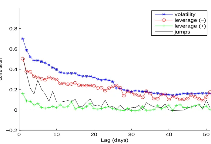
Figure 1 shows, for the S&P 500 series studied in this paper, the lagged correlation function

between the two-scale estimator TSRV_{t and} TSRV_{t−h itself, negative returns, positive returns}

and bJ_{t−h. The autocorrelation of} TSRV_{t decays very slowly, as it is well known. The lagged}

correlation betweenTSRV_{tand negative returns shows the leverage effect: volatility is correlated}

with lagged negative returns. Figure 1 also shows that the impact of negative returns on future

volatility is slowly decaying as well. Also jumps have a positive and large impact (as large as

the negative returns whenh= 1), which however decays more rapidly. Finally, positive returns

have a very small and negligible impact on future volatility.

The slowly decaying impact of negative returns might well be a by-product of the slowly decaying

auto-correlation function of volatility. However, since the same phenomenon is not observed with

Realized volatility memory

0 10 20 30 40 50

−0.2 0 0.2 0.4 0.6 0.8

Lag (days)

correlation

volatility leverage (−) leverage (+) jumps

Figure 1: Lagged correlation function between past valuesYt−hand current, daily,

integrated variance estimates TSRV_{t as a function of h, withYt−h being}TSRV_t−h

itself, negative returns, positive returns and jumps quadratic variationbJ_t−h for the S&P500 futures from 28 April 1982 to 5 February 2009 (6,669 observations).

persistent, a possibility which has been seldom investigated so far.

Persistence in the leverage effect can be induced, in continuous time, by making the leverage

effect an explicit function of volatility, as in Bandi and Ren`o (2011b). Our reduced-form model,

which is in discrete time, explores an alternative possibility. We follow Corsi (2009) in modeling

the slowly decaying auto-correlation function by means of a heterogeneous structure induced

by a volatility cascade, and we extend this structure to negative returns and jumps.

2.2 The LHAR-CJ model

Combining heterogeneity in realized volatility, leverage, and jumps we construct the Leverage

it is common in practice, we use daily, weekly and monthly frequencies. Then, using variable

specified in logs, we introduce averaged variables, which are defined over an integer numberh

of days as (jumps are aggregated instead of averaged):

logVb(_th)₌ 1

h

h

X

j=1

logVb_{t−j+1, log}Cb(_th)₌ 1

h

h

X

j=1

logCb_{t−j+1, r}(h)

t = 1 h h X j=1

rt−j+1, bJ (h)

t =

h

X

j=1

b J_t−j+1.

To model the leverage effect at different frequencies, we define r(_th)− = min(r_t(h),0). The

pro-posed model reads:

logVb(_th₊)_{h =c + β}(d)_logCb_t+β(w)_logbC(5)_{t +β}(m)_logbC(22)_t

+ α(d)_{log(1 +bJ}

t) +α(w)log(1 +bJ (5)

t ) +α(m)log(1 +bJ (22)

t ) (2.4)

+ γ(d)r−_t +γ(w)r(5)_t −+γ(m)r(22)_t −+ε(_th₊)_h,

with real parameters {c, β(d,w,m)_{, α}(d,w,m)_{, γ}(d,w,m)_{} and where ε}(h)

t is IID noise. Model (2.4)

nests other models which have been successfully used for realized volatility. When α(d,w,m) ₌

γ(d,w,m)_{= 0 andCb}

t=Vbt, the model becomes the HAR model of Corsi (2009). Whenγ(d,w,m)=

0, we get the HAR-CJ model proposed by Andersen et al. (2007) which separately include

continuous and discontinuous component as explanatory variables. When α(d,w,m) _{= 0 and}

b

C_t=Vb_{t the model is referred to as the LHAR model. The model can also be specified directly}

forVb_{t and for} q

b

V_{t, as in Andersen et al. (2007) and Corsi et al. (2010).}

We estimate model (2.4) and its variants, with h ranging from 1 to 22 to make multiperiod

predictions, by OLS with Newey-West covariance correction for serial correlation.

3

Empirical evidences

The purpose of this section is to empirically analyze the performance of the LHAR-CJ model

Jump Contribution to Total Variation

1990

2000

0%

10%

20%

30%

40%

50%

60%

Year

3−month window

1−year window

Figure 2: Percentage contribution of daily jump to total quadratic variation mea-sured over a moving window of 3-month (dotted line) and 1-year (solid line) for the S&P500 futures from 28 April 1982 to 5 February 2009 (6,669 observations) excluding the October 1987 crash. TheC-Tzstatistics is computed with a confidence interval

α= 99.9%.

span of almost 28 years of high frequency data for the S&P 500 futures from 28 April 1982

to 5 February 2009. We leave out from the sample the week of the 1987 October crash (when

included, results are qualitatively very similar but less clear-cut) and days with less than 500

trades. We are left with 6,669 days. All the quantities of interest are computed on an annualized

base. Figure 2 reports the relative contribution of the quadratic variation of jumps with respect

to total quadratic variation, computed on a 3-month and 1-year moving window. In line with

the results in Andersen et al. (2007) and Huang and Tauchen (2005) we find a jump contribution

varying between 2% and 30% of total variation (with an overall sample mean of about 6%).

3.1 In-sample analysis

The results of the estimation of the LHAR-CJ on the S&P500 sample with h = 1,5,10,22

Newey-S&P500 LHAR in-sample regression, period 1982–2009

Variable One day One week Two weeks One month

c 0.442* 0.549* 0.662* 0.858*

(10.699) (9.258) (8.525) (7.756)

b

C _{0.307* 0.201* 0.154* 0.116*}

(16.983) (14.158) (12.984) (10.590)

b

C(5) _{0.369* 0.359* 0.332* 0.286*}

(13.908) (11.251) (9.166) (6.784)

b

C(22) _{0.222* 0.319* 0.370* 0.415*}

(10.958) (10.913) (10.198) (9.344)

bJ _{0.043* 0.020* 0.017* 0.012*}

(7.057) (4.453) (4.485) (3.804)

bJ(5) _{0.011* 0.013* 0.011* 0.010}

(3.373) (3.112) (2.256) (1.913)

bJ(22) _{0.005* 0.008* 0.010* 0.014*}

(2.199) (2.106) (2.205) (2.336)

r− -0.007* -0.005* -0.004* -0.003*

(-9.669) (-10.435) (-8.298) (-5.518)

r(5)− -0.008* -0.006* -0.008* -0.007*

(-4.412) (-3.059) (-4.012) (-3.472)

r(22)− -0.009* -0.012* -0.009 -0.004

(-2.845) (-2.314) (-1.481) (-0.467)

R2 0.7664 0.8137 0.8030 0.7629 HRMSE 0.2168 0.1692 0.1699 0.1796

Table 1: OLS estimates of LHAR-CJ regressions, model (2.4), for the S&P500 futures from 28 April 1982 to 5 February 2009 (6,669 observations). The LHAR-CJ model is estimated with h = 1 (one day), h = 5 (one week), h = 10 (two weeks) and

h = 22 (one month). The significant jumps are computed using a critical value of

α= 99.9%. Reported in parenthesis aret-statistics based on Newey-West correction withL= 2 + 2hnumber of lags and Bartlett kernel. A star denotes 95% significance.

West robust t-statistic. The forecasts of the different models are evaluated on the basis of

the adjustedR2 of the regressions, and the heteroskedasticity-adjusted root mean square error

(HRMSE) proposed by Bollerslev and Ghysels (1996).

As usual, all the coefficients of the three continuous volatility components are positive and, in

general, highly significant. The impact of daily and weekly volatility decreases with the

forecast-ing horizon of future volatility, while the impact of monthly volatility increases. The coefficient

double than that of daily volatility on future monthly volatility. This finding is consistent with

Corsi (2009).

Estimation of model (2.4) also reveals the strong significance (with an economically sound

negative sign) of the negative returns at all the daily, weekly and monthly aggregation frequency,

which unveils a heterogeneous structure in the leverage effect as well. Not only daily negative

returns affect the next day volatility (the well-know leverage effect) but, in addition, also the

negative returns of the past week and past month have an impact on forthcoming volatility.

This novel finding suggests that the market might aggregate daily, weekly and monthly memory,

observing and reacting to price declines happened in the past week and month, revealing a

persistent leverage effect.

A similar heterogeneous structure is present in the impact of jumps on future volatility. However,

while the daily and weekly jumps are highly significant and positive, their impact decreases with

the forecasting horizon at a fast rate. The monthly jump component is also slightly significant

over all forecasting horizons, with its impact increasing with the horizon.

Figure 3 shows the Mincer-ZarnowitzR2 _{for different models at various horizons, which obtaines}

its maximum at one week. Moreover, Figure 3 shows unambiguously that the inclusion of

both the heterogeneous jumps and the heterogeneous leverage effects considerably improves the

forecasting performance of the S&P 500 volatility at any forecasting horizon. In particular,

the inclusion of heterogeneous leverage effect provides the most relevant overall benefit in the

in-sample performance. We confirm this result out-of-sample in Section 3.6.

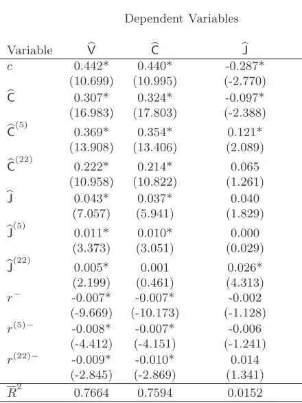
3.2 Forecasting jumps and continuous volatility

Following Busch et al. (2011), we can use the continuous and jumps component of total quadratic

variation as dependent variables as well, and investigate the possibility of forecasting them

In-sample Mincer-Zarnowitz

R

0

5

10

15

20

0.74

0.76

0.78

0.8

0.82

horizon (days)

HAR

HAR−CJ

LHAR−CJ

Figure 3: R2 of Mincer-Zarnowitz regressions for static in sample one-step ahead forecasts for horizons ranging from 1 day to 1 month of the S&P500 futures from 28 April 1982 to 5 February 2009 (6,669 observations). The forecasting models are the standard HAR with only heterogeneous volatility, the HAR-CJ with heterogeneous jumps and the LHAR-CJ model.

variation as:

logCb(_t+h)_{h =c + β}(d)_logbC_t+β(w)_logCb(5)_{t +β}(m)_logCb(22)_t

+ α(d)_{log(1 +bJ}

t) +α(w)log(1 +bJ (5)

t ) +α(m)log(1 +bJ (22)

t ) (3.1)

+ γ(d)r−_t +γ(w)r(5)_t −+γ(m)r(22)_t −+ε(_t+h)_h,

and the LHAR-J-CJ model for forecasting jumps as:

log(1 +bJ(h)

t+h) =c + β(d)logCbt+β(w)logCb (5)

t +β(m)logCb (22) t

+ α(d)log(1 +bJ_{t) +α}(w)_{log(1 +}bJ(5)_{t ) +α}(m)_{log(1 +}bJ(22)_{t ) (3.2)}

Corresponding models withα(d,w,m)_{= 0 andCb}

t=Vbton the right-hand side are named

LHAR-C and LHAR-J respectively. Estimation results for the daily horizon (h = 1) are presented

in Table 2. We can see that, as already recognized in the literature, the jump component

is essentially unpredictable, with an adjusted R2 of just 1.52%. We find a strong significant

impact on future jumps only for the monthly jump component, which is a clear indication of

jump clustering. Also daily and weekly volatilities are significant, but with opposite signs. The

impact of monthly jumps on bC_{t is instead not significant, confirming that the impact of jumps}

on volatility is quite transitory in nature.

While the inability of forecasting jumps has been signaled also by Busch et al. (2011), they find,

contrary to our analysis, that the impact of daily jumps on the future daily continuous quadratic

variation is significantly negative, a result which would imply, on average, a volatility decrease

after a jump. Corsi et al. (2010) show that this result is induced by the small-sample bias of

bipower variation measures. Building on their work, we use threshold bipower variation and

uncover the positive (and transitory) impact of jumps on future volatility also in the presence

of a persistent leverage effect.

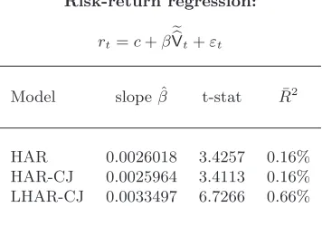
3.3 Risk-return trade-off

Our volatility forecasts can also be evaluated in term of the implied risk-return trade-off, since

economic theory posits that there should be a positive relation between returns and perceived

risk. The literature on the risk-return trade-off is very large. Recent research on this topic

in-cludes Ghysels et al. (2005); Christensen and Nielsen (2007); Bandi and Perron (2008); Bollerslev

et al. (2008). Here we use as a measure of risk the daily volatility forecast of i) the standard

HAR model, ii) the HAR-CJ model and iii) the LHAR-CJ model. All models are specified in the

logarithmic form. We regress the return on the variance forecastsVeb_{t, that is on the exponential}

of the logarithmic forecasts logVeb_{t. Estimation results, obtained via OLS, are shown in Table 3.}

LHAR-CJ, LHAR-C-CJ and LHAR-J-CJ regression

Dependent Variables

Variable Vb Cb bJ

c 0.442* 0.440* -0.287*

(10.699) (10.995) (-2.770)

b

C 0.307* 0.324* -0.097*

(16.983) (17.803) (-2.388)

b

C(5) _{0.369* 0.354* 0.121*}

(13.908) (13.406) (2.089)

b

C(22) 0.222* 0.214* 0.065

(10.958) (10.822) (1.261)

bJ 0.043* 0.037* 0.040

(7.057) (5.941) (1.829)

bJ(5) _{0.011* 0.010* 0.000}

(3.373) (3.051) (0.029)

bJ(22) 0.005* 0.001 0.026*

(2.199) (0.461) (4.313)

r− -0.007* -0.007* -0.002

(-9.669) (-10.173) (-1.128)

r(5)− -0.008* -0.007* -0.006

(-4.412) (-4.151) (-1.241)

r(22)− _{-0.009* -0.010* 0.014}

(-2.845) (-2.869) (1.341)

R2 0.7664 0.7594 0.0152

Table 2: OLS estimate for the LHAR-CJ model using as dependent variable logVb_t, logCb_{t, log(1 +}bJ_{t), daily forecasting horizon, for the S&P500 futures from 28 April}

1982 to 5 February 2009 (6,669 observations). The significant jumps are computed using a critical value ofα= 99.9%. Reported in parenthesis aret-statistics based on Newey-West correction withL= 2 + 2hnumber of lags and Bartlett kernel. A star denotes 95% significance.

until 2002. With all models, we find a significant impact of volatility forecasts on returns which

is compatible with economic theory, even if we have a very low R2_{, as it is common in this}

kind of applications. The inclusion of jumps is not benefitial to return forecasting. Instead,

the inclusion of the leverage component increases the slope coefficient and almost doubles the

significance of the effect. Similar results are obtained regressingrton

q eb

V_{t, or replacing}Veb_twith

Risk-return regression:

rt=c+βebVt+εt

Model slope ˆβ t-stat R¯2

HAR 0.0026018 3.4257 0.16%

HAR-CJ 0.0025964 3.4113 0.16%

LHAR-CJ 0.0033497 6.7266 0.66%

Table 3: OLS estimates of the regression of daily returns on daily variance forecasts

e b

V_tobtained with different models

3.4 Is leverage effect induced by jumps?

An open research question is whether, and to which extent, the leverage effect is induced by

jumps, see e.g. Bandi and Ren`o (2011a). In our setting, we investigate this issue by separating

the daily jump contribution to quadratic variation in a positive and negative part. To this

purpose, we define:

b J+

t =bJt·I{rt>0}

b

J−_{t =}bJ_t·I{r t<0}

and we insertbJ+

t andbJ

−

t in the LHAR model in place ofbJt, denoting by LHAR-CJ+ the newly

obtained model. We also estimate the HAR-CJ+ model, which is the same without leverage

terms. Results are reported in Table 4. Given the evidence provided by Todorov and Tauchen

(2011) and Bandi and Ren`o (2011a), with different statistical methods, of a strong negative

correlation between price and volatility jumps, we expect the coefficient onbJ−_{t to be larger than}

that onbJ+_{t .}

When we estimate the HAR-CJ+_{model, this is exactly what we find: the coefficient on negative}

jumps is almost double than that of positive jumps, and this is true for all the considered

HAR-CJ+ _regression

1 day 1 week 2 weeks 1 month

c 0.232* 0.377* 0.505* 0.747*

(5.774) (6.217) (6.418) (6.736)

b

C 0.398* 0.265* 0.214* 0.165*

(21.521) (18.225) (16.084) (12.442)

b

C(5) 0.366* 0.368* 0.346* 0.291*

(13.889) (11.697) (9.750) (7.327)

b

C(22) _{0.190* 0.291* 0.338* 0.390*}

(9.470) (9.743) (9.059) (8.875)

b

J+ 0.044* 0.018* 0.016* 0.013*

(6.099) (3.264) (3.000) (2.538)

b

J− 0.074* 0.040* 0.039* 0.027*

(6.909) (6.833) (6.658) (5.351)

b

J(5) _{0.009* 0.012* 0.010* 0.010}

(2.645) (2.724) (2.028) (1.799)

b

J(22) 0.005 0.007 0.009* 0.014*

(1.845) (1.875) (2.026) (2.242)

-R2 0.7543 0.8060 0.7960 0.7582

HRMSE 0.2201 0.1721 0.1722 0.1812

LHAR-CJ+_regression

1 day 1 week 2 weeks 1 month

c 0.442* 0.549* 0.661* 0.858*

(10.724) (9.277) (8.531) (7.778)

b

C _{0.307* 0.201* 0.154* 0.116*}

(16.972) (14.185) (13.007) (10.608)

b

C(5) 0.369* 0.359* 0.332* 0.286*

(13.885) (11.237) (9.144) (6.777)

b

C(22) _{0.222* 0.319* 0.370* 0.415*}

(10.914) (10.905) (10.183) (9.336)

b

J+ 0.044* 0.018* 0.015* 0.012*

(6.176) (3.182) (2.819) (2.395)

b

J− 0.043* 0.019* 0.020* 0.011*

(4.598) (3.387) (3.633) (2.285)

b

J(5) _{0.011* 0.013* 0.011* 0.010}

(3.372) (3.110) (2.254) (1.914)

b

J(22) 0.005* 0.008* 0.010* 0.014*

(2.200) (2.104) (2.203) (2.337)

r− -0.007* -0.005* -0.004* -0.003*

(-9.772) (-10.057) (-7.804) (-5.341)

r(5)− -0.008* -0.006* -0.008* -0.007* (-4.409) (-3.068) (-4.020) (-5.341)

r(22)− _{-0.009* -0.012* -0.008 -0.004}

(-2.844) (-2.315) (-1.484) (-0.467)

R2 0.7664 0.8137 0.8030 0.7629

HRMSE 0.2168 0.1692 0.1698 0.1796

Table 4: OLS estimate for the LHAR-CJ+_{and HAR-CJ}+_{model in which we separate}

daily jumps in positive and negative, for the S&P500 futures from 28 April 1982 to 5 February 2009 (6,669 observations). The models are estimated with h = 1 (one day),h= 5 (one week),h= 10 (two weeks) andh= 22 (one month). The significant jumps are computed using a critical value of α = 99.9%. Reported in parenthesis aret-statistics based on Newey-West correction withL= 2 + 2hnumber of lags and Bartlett kernel. A star denotes 95% significance.

LHAR-CJ+ _{model, which includes all the leverage terms (which are also affected by the jump}

component), the impact of positive and negative jumps is estimated to be roughly the same,

again at all the considered horizons. Our interpretation of this result is that the number of

co-jumps is likely too small to allow for the joint detection of the continuous leverage effect and

3.5 Robustness to other volatility measures

In the literature many volatility measures have been proposed as explanatory variables for the

volatility dynamics. Forsberg and Ghysels (2007) proposed the use of realized absolute variation

(RAV) which shows a more persistent dynamics than realized volatility being more robust to

microstructure noise and jumps. The range, i.e. the difference between the highest and the

lowest price within a day, has also been found to be significant by many authors, see e.g.

Brandt and Jones (2006) and Engle and Gallo (2006). Recently, Barndorff-Nielsen et al. (2010)

proposed the realized semivariance as the sum of square negative returns to capture the impact

on volatility of downward price pressures. Visser (2008) combines RAV and semivariance by

taking the sum of negative absolute squared returns.

In the spirit of Forsberg and Ghysels (2007), we compare the relative explanatory power of

different volatility measures by estimating a set of models (for space concerns we limit ourselves

to the one day horizon) obtained by adding explanatory variables to model (2.4). Estimation

results are reported in Table 5. In line with previous literature, we find that the realized absolute

variation (RAV) computed at 5-minute frequency and the range have a significant impact on

future volatility. However, they seem to be mainly substitutes for continuous volatility and

jumps, which is not totally surprising since they are estimators (though noisy) of total quadratic

variation. Indeed, for instance, when the range replaces the jumps (LHAR-Range model, not

reported), the coefficients of daily continuous volatility almost halves. The adjusted R2 of the

two competing regressions (LHAR-Range and LHAR-CJ) is practically the same. When the

range is inserted together with the jumps (LHAR-CJ-Range), both the coefficients of daily

volatility and jumps decrease, although they remain highly significant. The significance of the

heterogeneous leverage effect is instead unaffected by the presence of RAV and range. We

thus conclude that the RAV and the range, while partially proxying for both volatility and

jumps, are also able to capture some other (small) effect which is not captured by the other

only marginally. The realized semivariance (semiRV) of Barndorff-Nielsen et al. (2010) and

the downward absolute power variation of Visser (2008) (semiRAV) have a weaker impact.

Realized semivariance and semi-power-variation are significant in explaining future volatility,

and, again, they are correlated with both the daily two-scale estimator and the jumps (typically

depleting the significance of the corresponding coefficients without totally removing it), while

unrelated with the leverage. However, their contribution to the model performance is not

significant (as measured by the Diebold-Mariano test). Moreover, when they are included in

the all-encompassing model they both remain insignificant.

Summarizing, the results of this section show that when the other volatility measures proposed

in the literature are inserted in the baseline LHAR-CJ model they either do not contribute

significantly or only marginally contribute to the performance of the model. Moreover, they

mainly act as substitutes of continuous volatility and jumps. Hence, we conclude the LHAR-CJ

model seems to capture the main determinants of volatility dynamics.

3.6 Out-of-sample analysis

In this section, we evaluate the performance of the LHAR-CJ model on the basis of a genuine

out-of-sample analysis. For the out-of-sample forecast of Vb_{t on the [t, t+h] interval we keep}

the same forecasting horizons ranging from one day to one month and re-estimate the model

at each day t on an increasing window of all the observation available up to time t−1. The

out-of-sample forecasting performance for logVb_{t in terms of Mincer-Zarnowitz R}2 _{is reported}

in Figure 4, together with the Diebold-Mariano test computed for the HRMSE loss function at

all the considered horizons.

The superiority of the LHAR-CJ model at all horizons, with respect to the HAR and the

HAR-CJ model, is statistically significant, validating the importance of including both the

heterogeneous leverage effects and jumps in the forecasting model. The out-of-sample exercise

S&P500 in-sample estimates, period 1982–2009 Variable LHAR-CJ LHAR- CJ-RAV LHAR- CJ-Range LHAR- CJ-SemiRV LHAR- CJ-SemiRAV LHAR-CJ-All

const 0.442* 0.593* 0.444* 0.470* 0.554* 0.616*

(10.699) (12.419) (10.860) (11.029) (9.869) (8.914)

b

C _{0.307* 0.116* 0.207* 0.249* 0.252* 0.085*}

(16.983) (3.355) (10.035) (9.588) (9.489) (2.449)

b

C(5) _{0.369* 0.374* 0.384* 0.372* 0.372* 0.389*}

(13.908) (14.125) (14.568) (14.074) (14.032) (14.693)

b

C(22) 0.222* 0.221* 0.223* 0.223* 0.222* 0.223*

(10.958) (10.943) (11.071) (11.003) (10.963) (11.035)

b

J _{0.043* 0.018* 0.024* 0.033* 0.037* 0.010}

(7.057) (2.519) (3.893) (4.850) (5.620) (1.331)

b

J(5) 0.011* 0.012* 0.012* 0.011* 0.011* 0.012*

(3.373) (3.717) (3.789) (3.409) (3.413) (3.959)

b

J(22) 0.005* 0.006* 0.005* 0.006* 0.006* 0.006*

(2.199) (2.334) (2.207) (2.266) (2.277) (2.329)

r− _{-0.007* -0.007* -0.006* -0.006* -0.006* -0.005*}

(-9.669) (-10.156) (-8.193) (-8.197) (-7.792) (-5.630)

r(5)− _{-0.008* -0.007* -0.008* -0.008* -0.008* -0.008*}

(-4.412) (-4.147) (-4.847) (-4.368) (-4.278) (-4.582)

r(22)− _{-0.009* -0.009* -0.009* -0.010* -0.010* -0.010*}

(-2.845) (-2.687) (-2.868) (-2.980) (-2.951) (-2.853)

RAV 0.185* 0.077

(6.533) (1.867)

Range 0.088* 0.086*

(9.364) (7.911)

SemiRV 0.058* -0.011

(3.305) (-0.330)

SemiRAV 0.054* 0.056

(3.141) (1.455)

R2 0.7664 0.7681 0.7696 0.7668 0.7668 0.7704

HRMSE 0.2168 0.2158* 0.2148* 0.2165 0.2165 0.2142*

DM (2.7060) ( 4.6323) (1.5020 ) (1.8539 ) (4.6778)

The superiority of the HAR-CJ model vs the HAR model is instead milder, but the reason

is that the improvements appear only in days which follow a jump (368 out of 6,669), and

thus on a small subsample. However, it is important to note that the inclusion of the jump

component helps also in forecasting longer horizon volatility, see the results in the web appendix

and Andersen et al. (2007).

4

Continuous-time models

The main motivation of this section is to provide a continuous-time model which delivers the

stylized facts documented in the previous sections and captured by the newly proposed

discrete-time model. Such a continuous-discrete-time model would then, at the same discrete-time, not only provide a

more accurate statistical representation of the data, but also bridge the gap between continuous

and discrete time modelling. Since the inception of the GARCH literature, indeed, volatility

forecasting is mostly set up in discrete time, and the LHAR-CJ model is no exception. However,

models used in practice, e.g. for option pricing, are often specified in continuous time. In the

literature, the link between GARCH-like models and continuous time models is well established,

see e.g. Nelson (1990); Duan (1997); Corradi (2000). However, the link between continuous-time

models and HAR-like models is unclear.

We achieve this goal by estimating continuous-time models via indirect inference (Gourieroux

et al. 1993; see Bollerslev et al. 2006 for an application similar to ours) using the (L)HAR(-CJ)

specification as auxiliary model. The idea of the indirect inference approach is to estimate the

auxiliary model both on actual data and on data simulated from the structural model, and then

to minimize the distance (labelled by χ2_{), as a function of the structural model parameters,}

between the estimated coefficients weighted with the inverse variance-covariance matrix of the

estimates. Details are provided in the Web Appendix.

Out-of-sample Mincer-Zarnowitz

R

0 5 10 15 20

0.74 0.76 0.78 0.8 0.82

horizon (days)

HAR HAR−CJ LHAR−CJ

Out-of-sample Diebold-Mariano test

0 5 10 15 20

0 2 4 6 8 10 12

HAR vs HAR−CJ HAR vs LHAR−CJ HAR−CJ vs LHAR−CJ

generated by a long-memory model. For this reason, we start by estimating the Comte and

Renault (1998) continuous-time model:

dXt=σtdWt,

dlogσt=k(ω−logσt)dt+ηdWt(d),

(4.1)

where Wt is a standard Brownian motion and dWt(d) is an independent fractional Brownian

motionwith memory parameterd∈[0,0.5] (ensuring stationarity). The valued= 0 corresponds

to the standard Brownian motion, while higher d corresponds to higher memory in the time

series. Estimation of model (4.1) has only been performed, to the best of our knowledge,

in Casas and Gao (2008) using spectral methods. For simulation studies, see Nielsen and

Frederiksen (2008) and Rossi and Spazzini (2010). A discrete time specification of model (4.1)

is instead estimated more routinely, see e.g. Comte and Renault (1996) and Christensen and

Nielsen (2007). To assess the impact on the results of the fractional difference parameterd, we

first estimate model (4.1) for different fixed values d, and then estimate the four parameters

(k, ω, η, d) jointly.

The results, reported in Table 6, show that model (4.1) is substantially unable to reproduce the

coefficients of the HAR model. The best fit is obtained with a value of d= 0.491 very close to

non-stationarity. However, even for this fit, the implied daily coefficient of the HAR model is

still too high, and the implied weekly coefficient is still too low. To understand the motivation

of this failure, it is interesting to look at the estimates obtained for fixed and increasing values

ofd. Whend= 0, the model is assimilable to anAR(1) specification and thus is unsurprisingly

unable to reproduce the HAR coefficients. As d increases, persistence comes from two terms:

the mean-reverting termk(ω−logσ_t2)dt and the fractional Brownian motionηdW_t(d). However,

these two components can vary only in a rigid fashion. For example, when d increases, the

mean-reversion parameter k has to increase sharply because of the mean reversion observed

Structural model:

dlogσt=k(ω−σt)dt+ηdWt(d)

parameter estimates

d= 0 d= 0.1 d= 0.2 d= 0.3 d= 0.4 d= 0.49 unconstrainedd k 0.144 0.325 0.750 1.917 7.706 145.081 144.853

ω −0.166 −0.218 −0.268 −0.290 −0.313 −0.446 −0.447

η 0.248 0.272 0.352 0.625 2.512 118.350 123.746

d 0.000 0.100 0.200 0.300 0.400 0.490 0.491

χ2 1109.4187 1137.1615 931.5612 527.4070 178.8777 43.2839 42.6094

Auxiliary model:

logCb_t+1=c+β(d)_logCb_t+β(w)_logbC(5)_{t +β}(m)_logCb(22)_{t +εt}

parameter estimated implied

d= 0 d= 0.1 d= 0.2 d= 0.3 d= 0.4 d= 0.49 unconstrainedd c 0.208 0.661 0.875 1.019 0.966 0.688 0.440 0.436

β(d) _{0.388 0.913 0.877 0.756 0.575 0.449 0.420 0.421} β(w) 0.368 −0.044 −0.083 −0.059 0.057 0.203 0.281 0.281

β(m) _{0.203 0.004 0.035 0.099 0.173 0.209 0.211 0.211} σ2

ε 0.198 0.188 0.191 0.195 0.198 0.199 0.198 0.197

Table 6: Estimates (daily units) via indirect inference of the long memory model (4.1) using the HAR model as auxiliary model, and implied HAR coefficients.

k∞=ηd/k remains approximately constant when changingd. This rigidity makes model (4.1)

unable to reproduce the HAR model.

Given the failure of the single-factor long memory model, we get inspiration from the very

nature of the HAR model, which reproduces a slowly decaying autocorrelation function via the

aggregation of different frequencies, and estimate affine multi-factor models with jumps:

dXt= N

X

i=1

q

Vi

tdWti+dJtX

dVi

t =κi(ωi−Vti)dt+ηi

p

Vi

tdWti+N +dJti i= 1, . . . , N

corr(dWi_{, dW}i+N_{) =ρ} i

(4.2)

whereW1, . . . , W2N _{is a multivariate (possibily correlated) Brownian motion andJ={J}X_{, J}1_,

Structural model:

dXt= p

V1 t dW

1 t +

p

V2 tdW

2 t

dVt1=κ1(ω−Vt1)dt+η1 p

V1 tdWt3

dVt2=κ2(ω−Vt2)dt+η2 p

V2 tdWt4

parameter estimates

κ1 2.1461 κ2 0.0042 ω 0.4497

η1 0.8513 η2 0.3110 χ2 0.0000026

Auxiliary model:

logCb_t+1=c+β(d)_logCb_t+β(w)_logbC(5)_{t +β}(m)_logCb(22)_{t +εt}

parameter estimated implied

c 0.208 0.208

β(d) _{0.388 0.388} β(w) _{0.368 0.368} β(m) _{0.203 0.203} σε2 0.198 0.198

Table 7: Estimates (daily units) via indirect inference of model (4.2) withN= 2 and

ω1=ω2=ω, using the HAR model as auxiliary model, and implied HAR coefficients.

jump sizes in the prices and exponential jump sizes in volatility. In the case of no jumps, when

N = 1, this is the well known Heston (1993) model; Duffie et al. (2000) and Pan (2002) include

jumps as in the Eraker et al. (2003) model considered earlier. WithN = 2, this model has been

used for example in Bates (2000) and, more recently, by Christoffersen et al. (2009).

When using the HAR model as auxiliary model, we set N = 2, ρi = 0, J= 0 and to achieve

identification ω1 = ω2 = ω. Corresponding estimates, together with the implied HAR

coeffi-cients, are reported in Table 7. Contrary to the single-factor model with fractional Brownian

motion, the two-factor model is perfectly able to reproduce the HAR coefficients, obtaining an

objective function χ2 close to zero. Estimates are compatible with those typically encountered

in the literature: the fit implies the presence of a fast mean-reverting factor with a half-life less

than one day, and a slowly mean-reverting factor with a half-life of nearly 200 days. The

super-position of these two frequencies produces the desired effect in terms of volatility persistence.

Lieberman and Phillips (2008) suggest that also the usage of integrated volatility measures

produces a longer memory than that implied in the dynamics of spot volatility. Our result

also explains why multi-factor model works so well in describing the dynamics of options, see

e.g. Bates (2000), since they are able to reproduce the volatility dynamics under the natural

is specified directly with a model similar to HAR: an attempt in this direction is the paper

of Corsi et al. (2011), which develops an option pricing model with HAR volatility dynamics

providing remarkable pricing performance with a single volatility factor. Finally, two volatility

factors have also been shown to be priced in the cross-section of expected returns, see Adrian

and Rosenberg (2008).

When the auxiliary model is LHAR, the natural approach is to allow for nonzero correlation

coefficients to introduce a leverage effect, again settingJ_{= 0. We report estimates of the}

two-factor model with leverage effect in Table 8. When fitting the two-two-factor model using the LHAR

model as auxiliary model, we findρ1 >0, that is a positive correlation coefficient between the

fast mean-reverting volatility factor and returns, while ρ2 is negative. This fact is not totally

surprising since it echoes the results of Chernov et al. (2003) and Bollerslev et al. (2006), who

also estimate (among other models) a two-factor affine model on S&P500 returns via efficient

method of moments (using an auxiliary GARCH model) and find the correlation coefficient

associated to the fast mean-reverting volatility factor to be positive.

In presence of two factors, the interpretation of the leverage effect is not trivial since, as also

Chernov et al. (2003) explain, the average leverage can be negative even with a positive

correla-tion coefficient. However, the reason why a positive correlacorrela-tion arises with the fastest volatility

factor remained unclear. Figure 5 can help to provide a possible explanation for this occurrence.

We simulate model (4.2) with the coefficients estimated in Table 7, and we varyρ1(withρ2 = 0)

and ρ2 (with ρ1 = 0) to evaluate the impact of the introduced correlations on the LHAR

coef-ficients. When ρ1 (the leverage effect of the fast mean-reverting factor) is different from zero,

the impact of daily negative returns on future volatility follows the sign ofρ1, but the opposite

hold for the impact of weekly and monthly negative returns. For example, whenρ1 is negative,

we findγ(d)_{<0 butγ}(w)_{, γ}(m)_{>0. This is due to anovershootingeffect: a positive correlation}

at a higher frequency becomes negative at a slower one and viceversa. However, for the slowly

Structural model:

dXt= p

V1 t dWt1+

p

V2 tdWt2+

p

V3

t dWt3+cXdNt

dVt1=κ1(ω1−Vt1)dt+η1 p

V1 t dW

4

t +cσdNt

dVt2=κ2(ω2−Vt2)dt+η2 p

V2 t dW

5 t

dVt3=κ3(ω3−Vt3)dt+η3 p

V3 t dW

6 t

corr(dW1_{, dW}4_{) =ρ} 1 corr(dW2, dW5) =ρ2 corr(dW3, dW6) =ρ3

Nt∼P oisson(λt), cX∼ N(0, σJ2), cσ ∼exp(µσ)

parameter two factor three factor three factor with jumps

κ1 8.1088 6.7647 5.7233 κ2 0.0003 0.6556 0.8390

κ3 − 0.0036 0.00004

ω1 0.3030 0.2480 0.2468 ω2 0.5165 0.1348 0.1740

ω3 − 0.1894 0.1311

η1 1.6348 2.0128 1.8970 η2 0.3748 0.3880 0.4137

η3 − 0.2849 0.3412

ρ1 0.9847 0.3201 0.5040 ρ2 −0.9807 −0.9949 −0.8947 ρ3 − −0.9173 −0.9714

λ − − 0.0129

σJ − − 0.0254

µσ − − 0.1420

χ2 123.301 0.221 28.369

Auxiliary model:

logCb_t+1=c+β(d)_logCb_t+β(w)_logCb(5)_{t +β}(m)_logbC(22)_{t +}

+γ(d)r−t +γ (w)

rt(5)−+γ (m)

rt(22)−+εt

parameter estimated two factor three factor

c 0.421 0.561 0.428

β(d) 0.299 0.238 0.302

β(w) _{0.366 0.530 0.358} β(m) _{0.236 0.105 0.239} γ(d) −0.007 −0.004 −0.007

γ(w) _{−0.008 −0.014 −0.008} γ(m) −0.009 −0.010 −0.010

σε2 0.187 0.188 0.187

Auxiliary model:

logVb_t+1=c+β(d)logbC_t+β(w)logbC(5)_t +β(m)logbC(22)_t +

α(d)log(1 +bJ_t)+α(w)_{log(1 +}bJ(5)_{t )+α}(m)_{log(1 +}bJ(22)_{t )+}

+γ(d)r−t +γ (w)

rt(5)−+γ (m)

rt(22)−+εt

parameter estimated three factor with jumps

c 0.446 0.384

β(d) _{0.304 0.306} β(w) _{0.369 0.349} β(m) 0.222 0.260

α(d) _{0.042 0.017} α(w) _{0.011 0.011} α(m) 0.005 −0.000

γ(d) _{−0.007 −0.006} γ(w) _{−0.008 −0.006} γ(m) _{−0.009 −0.014}

σε2 0.183 0.182

Table 8: Estimates (daily units) via indirect inference of model (4.2) with two and three factors, using the LHAR model as auxiliary model, and implied LHAR coeffi-cients.

weekly and monthly coefficients, with the impact increasing with the horizon. The effect of

introducing correlations on volatility coefficients is instead marginal. Thus, with positiveρ1 we

with a negativeρ2.

Using the two-factor model, this mechanism is able to reproduce the LHAR model only partially:

the signs are correct but the coefficients estimated on the data can be reproduced only to a

limited extent. In order to get a satisfactory agreement with the LHAR model, we need to

introduce a third factor (in this case, the parameters of the structural model are not identified).

Estimates of the three-factor model are again reported in Table 8, and they show that with

ρ1 >0 and ρ2, ρ3 <0 we can reproduce completely the LHAR model.

Finally, we include jumps in the structural model with the aim of reproducing the results of the

LHAR-CJ model. Extensive Monte Carlo analysis, not reported here for brevity but available

in the Web Appendix, shows that a possible mechanism explaining the significant impact of

jumps on future volatility is given by the presence of contemporaneous jumps in price and

volatility, a possibility which has been recently empirically confirmed by Todorov and Tauchen

(2011) and Bandi and Ren`o (2011a). For this reason, in our last estimation we introduce a

single Poisson process Nt with constant intensity λ, and we set dJX = cXdNt, dJ1 =cVdNt,

J2_=J3 _{= 0 withc}

X ∼ N(0, σJ2) andcV ∼exp(µσ), that is we introduce co-jumps in price and

in a single volatility factor, namely the less persistent (also in this case the structural model

is not identified). Estimation results are reported in Table 8 and indicate that introducing

co-jumps provides a reasonable fit of the LHAR-CJ model, since we are able to reproduce both

the short-range persistence of jumps and the long-range persistence of leverage.

Concluding, we have seen that the LHAR-CJ model, and some of its relevant restrictions, are

fully consistent with a multi-factor Markovian volatility model. While it is certainly outside

the scope of this paper to provide a thorough interpretation on the mechanism which generated

the stylized facts described by the estimated statistical models, both in discrete time and in

continuous time, a possible interpretation of the empirical results goes as follows. Volatility

is highly persistent, and this persistence can be generated by a superposition of factors with

−10 −0.5 0 0.5 1 0.2

0.4 0.6

rho (short term)

volatility coefficients

−1 −0.5 0 0.5 1

−0.02 −0.01 0 0.01 0.02

rho (short term)

leverage coefficients

−10 −0.5 0 0.5 1

0.2 0.4 0.6

rho (long term)

−1 −0.5 0 0.5 1

−0.02 −0.01 0 0.01 0.02

rho (long term) daily

weekly monthly

Figure 5: Sensitivity of the coefficients of the LHAR specification (top row: β

coefficients of volatility; bottom row: γ coefficients on negative returns) the value of the leverage coefficientsρ1 (correlation with the fastly mean reverting factor, left

column), when ρ2 = 0, and ρ2 (correlation with the slowly mean reverting factor,

right column), whenρ1= 0.

are only correlated to a fast-reverting volatility factor via the mechanism of co-jumps, so that

their impact can only be short-lived. On the contrary, negative returns are correlated to all

volatility factors through the correlation of the shocks. For this reason, negative returns can

have a long-span impact on volatility, thus producing a persistent leverage effect.

5

Conclusions

In this paper, we uncover new stylized facts about volatility dynamics. While it is well known

the forecasting power of past negative returns remains significant even when considering them

over long horizons. The data also suggest that past jumps are (positively) correlated with

current volatility, but the forecasting power of aggregated jumps is milder when the aggregation

horizon is large. We then specify, both in discrete and in continuous time, suitable models which

are able to capture these novel stylized facts along with the well estabilished volatility features.

In the first stage, we propose a new discrete-time model for realized volatility measures, the

LHAR-CJ model, which naturally identifies three main determinants of volatility dynamics,

namely heterogeneous lagged continuous volatility, heterogeneous lagged negative returns and

heterogeneous lagged jumps. We find that each of the components in the discrete-time model

plays a different role at different forecasting horizons, but all the three are highly significant

and neglecting each one of them is detrimental to the forecasting performance.

In the second stage, we look for continuous-time models which reproduce the very same stylized

facts which are captured by the discrete-time specification. This is achieved by using the

discrete-time model as a convenient statistical metric in an indirect inference framework. A

multi-factor Markovian specification is found to be consistent with the empirical results and

compatible with the LHAR-CJ. To reproduce the long-term impact of negative returns, all the

volatility factors have to be correlated with the price shocks, while to reproduce the transient

impact of jumps it is enough to correlate price jumps with the jumps of one volatility factor

only (co-jumps).

We conclude by noting that our discrete-time model is very simple to implement, as it does

not require sophisticated computational technique. The estimation of the model parameters

can be performed through a simple OLS regression, and the computation of the explanatory

variables is trivial. We think that, for all the aforementioned reasons, the LHAR-CJ model may

References

Adrian, T. and J. Rosenberg (2008). Stock returns and volatility: Pricing the short-run and long-run components of market risk. Journal of Finance 63(6), 2997–3030.

A¨ıt-Sahalia, Y. and L. Mancini (2008). Out of sample forecasts of quadratic variation. Journal of Economet-rics 147(1), 17–33.

Allen, D. E. and M. Scharth (2009). Modelling the volatility of the FTSE100 index using high-frequency data sets. In G. N. Gregoriou (Ed.),Stock Market volatility, pp. 419–440. Chapman & Hall/CRC.

Andersen, T., T. Bollerslev, and F. X. Diebold (2007). Roughing it up: Including jump components in the measurement, modeling and forecasting of return volatility. Review of Economics and Statistics 89, 701–720. Bali, T. and L. Peng (2006). Is there a Risk-Return Tradeoff? Evidence from High-Frequency Data. Journal of

Applied Econometrics 21, 1169–1198.

Bandi, F. and B. Perron (2008). Long-run risk-return trade-offs. Journal of Econometrics 143, 349–374. Bandi, F. and R. Ren`o (2011a). Price and volatility co-jumps. Working paper.

Bandi, F. and R. Ren`o (2011b). Time-varying leverage effects. Journal of Econometrics. Forthcoming.

Barndorff-Nielsen, O., S. Kinnebrock, and N. Shephard (2010). Measuring downside risk: Realised semivariance. InVolatility and Time Series Econometrics: Essays in Honor of Robert F. Engle. Oxford University Press. Barndorff-Nielsen, O. E. and N. Shephard (2004). Power and bipower variation with stochastic volatility and

jumps. Journal of Financial Econometrics 2, 1–48.

Bates, D. (2000). Post-’87 crash fears in the S&P 500 futures option market. Journal of Econometrics 94, 181–238.

Bollerslev, T., C. Gallant, U. Pigorsch, C. Pigorsch, and G. Tauchen (2006). Statistical assessment of models for very high frequency financial price dynamics. Unpublished Manuscript.

Bollerslev, T. and E. Ghysels (1996). Periodic autoregressive conditional heteroscedasticity. Journal of Business & Economic Statistics 14(2), 139–151.

Bollerslev, T., U. Kretschmer, C. Pigorsch, and G. Tauchen (2009). A Discrete-Time Model for Daily S&P500 Returns and Realized Variations: Jumps and Leverage Effects. Journal of Econometrics 150(2), 151–166. Bollerslev, T., J. Litvinova, and G. Tauchen (2006). Leverage and Volatility Feedback Effects in High-Frequency

Data. Journal of Financial Econometrics 4(3), 353.

Bollerslev, T., G. Tauchen, and H. Zhou (2008). Expected stock returns and variance risk premia. Review of Financial Studies 22(11), 4463–4492.

Brandt, M. and C. Jones (2006). Volatility Forecasting With Range-Based EGARCH Models.Journal of Business and Economic Statistics 24(4), 470.

Busch, T., B. Christensen, and M. Nielsen (2011). The role of implied volatility in forecasting future realized volatility and jumps in foreign exchange, stock, and bond markets. Journal of Econometrics 160, 48–57. Campbell, J. Y. and L. Hentschel (1992). No news is good news: a asymmetric model of changing volatility in

stock returns. Journal of Financial Economics 31, 281–318.

Casas, I. and J. Gao (2008). Econometric estimation in long-range dependent volatility models: Theory and practice. Journal of econometrics 147(1), 72–83.

Chernov, M., R. Gallant, E. Ghysels, and G. Tauchen (2003). Alternative models for stock price dynamics.

Journal of Econometrics 116(1), 225–258.

Christensen, B. and M. Nielsen (2007). The effect of long memory in volatility on stock market fluctuations. The Review of Economics and Statistics 89(4), 684–700.

Christie, A. (1982). The stochastic behavior of common stock variances: value, leverage and interest rate effects.

Journal of Financial Economics 10, 407–432.

Christoffersen, P., S. Heston, and K. Jacobs (2009). The shape and term structure of the index option smirk: Why multifactor stochastic volatility models work so well. Management Science 55(12), 1914–1932.

Clark, T. and K. West (2007). Approximately normal tests for equal predictive accuracy in nested models.

Journal of Econometrics 138(1), 291–311.

Comte, F. and E. Renault (1996). Long memory continuous time models. Journal of Econometrics 73(1), 101–149.

Comte, F. and E. Renault (1998). Long memory in continuous-time stochastic volatility models. Mathematical Finance 8(4), 291–323.

Economet-rics 96, 145–153.

Corsi, F. (2005). Measuring and Modelling Realized Volatility: from tick-by-tick to long memory. Ph. D. thesis, PhD in Finance, University of Lugano.

Corsi, F. (2009). A simple approximate long-memory model of realized volatility. Journal of Financial Econo-metrics 7, 174–196.

Corsi, F., N. Fusari, and D. La Vecchia (2011). Realizing smiles: Pricing options with realized volatility.Journal of Financial Economics. Forthcoming.

Corsi, F., D. Pirino, and R. Ren`o (2010). Threshold bipower variation and the impact of jumps on volatility forecasting. Journal of Econometrics 159, 276–288.

Duan, J.-C. (1997). Augmented GARCH(p,q) process and its diffusion limit.Journal of Econometrics 79, 97–127. Duffie, D., J. Pan, and K. Singleton (2000). Transform analysis and asset pricing for affine junp-diffusions.

Econometrica 68, 1343–1376.

Engle, R. and G. Gallo (2006). A multiple indicators model for volatility using intra-daily data. Journal of Econometrics 131(1-2), 3–27.

Eraker, B., M. Johannes, and N. Polson (2003). The impact of jumps in volatility and returns. Journal of Finance 58, 1269–1300.

Fernandes, M., M. C. Medeiros, and M. Scharth (2009). Modeling and predicting the CBOE market volatility index. Working paper.

Forsberg, L. and E. Ghysels (2007). Why do absolute returns predict volatility so well? Journal of Financial Econometrics 5, 31–67.

Ghysels, E., P. Santa-Clara, and R. Valkanov (2005). There is a risk-return trade-off after all.Journal of Financial Economics 76(3), 509–548.

Glosten, L., R. Jagannathan, and D. Runkle (1989). On the relation between the expected value of the volatility of the nominal excess return on stocks. Journal of Finance 48, 1779–1801.

Gourieroux, C., A. Monfort, and E. Renault (1993). Indirect inference. Journal of Applied Econometrics 8, 85,118.

Heston, S. (1993). A closed-form solution for options with stochastic volatility with applications to bond and currency options. Review of financial studies 6, 327–343.

Huang, X. and G. Tauchen (2005). The relative contribution of jumps to total price variance.Journal of Financial Econometrics 3(4), 456–499.

Lieberman, O. and P. Phillips (2008). Refined inference on long memory in realized volatility. Econometric Reviews 27(1), 254–267.

Mancini, C. (2009). Non-parametric threshold estimation for models with stochastic diffusion coefficient and jumps. Scandinavian Journal of Statistics 36(2), 270–296.

Martens, M., D. van Dijk, and M. de Pooter (2009). Forecasting S&P500 volatility: Long memory, level shifts, leverage effects, day-of-the-week seasonality and macroeconomic announcements. International Journal of Forecasting 25, 282–303.

Muller, U., M. Dacorogna, R. Dav´e, R. Olsen, O. Pictet, and J. von Weizsacker (1997). Volatilities of different time resolutions - analyzing the dynamics of market components. Journal of Empirical Finance 4, 213–239. Nelson, D. (1990). ARCH models as diffusion approximations. Journal of Econometrics 45, 7–38.

Nielsen, M. O. and P. H. Frederiksen (2008). Finite sample accuracy and choice of sampling frequency in integrated volatility estimation. Journal of Empirical Finance 15, 265–286.

Pan, J. (2002). The jump-risk premia implicit in options: Evidence from an integrated time series study.Journal of Financial Economics 63, 3–50.

Rossi, E. and F. Spazzini (2010). Finite sample results of range-based integrated volatility estimation. Working Paper.

Scharth, M. and M. C. Medeiros (2009). Asymmetric effects and long memory in the volatility of Dow Jones stocks. International Journal of Forecasting 25, 304–327.

Todorov, V. and G. Tauchen (2011). Volatility jumps.Journal of Business and Economic Statistics 29, 356–371. Visser, M. (2008). Forecasting S&P 500 Daily Volatility using a Proxy for Downward Price Pressure. Working

Paper.