Multi-objective optimisation of constellation deployment using low-thrust propulsion

Multi-Objective Optimisation of Constellation

Deployment Using Low-Thrust Propulsion

Marilena Di Carlo

, Lorenzo Ricciardi

and Massimiliano Vasile

Department of Mechanical & Aerospace Engineering, University of Strathclyde, Glasgow, UK

This work presents an analysis of the deployment of future constellations using a com-bination of low-thrust propulsion and natural dynamics. Different strategies to realise the transfer from the launcher injection orbit to the constellation operational orbit are investi-gated. The deployment of the constellation is formulated as a multi-objective optimisation problem that aims at minimising the maximum transfer∆V, the launch cost and maximise at the same time the pay-off given by the service provided by the constellation. The paper will consider the case of a typical constellation with 27 satellites in Medium Earth Orbit and the use of only two launchers, one of which can carry a single satellite. It will be demonstrated that some strategies and deployment sequences are dominant and provide the best trade-off between peak transfer ∆V and monetary pay-off.

Nomenclature

a Semimajor axis i Inclination

Ω Right ascension of the ascending node µ Earth’s gravitational parameter R⊕ Earth’s radius

J2 Second zonal harmonic of the Earth’s gravitational potential

f Acceleration of the low-thrust engine β Elevation angle of the low-thrust vector α Semi-amplitude of the thrust arcs T oF Time of flight

∆V Variation of velocity required for the transfer

I.

Introduction

Satellite constellations are used for a wide range of applications and are deployed in different orbital regime around the Earth, according to their purpose. Navigation systems such as the Global Positioning System (GPS), the Russian Glonass and the Chinese BiDou are based on satellite constellations in Medium Earth Orbit (MEO). The European Space Agency is currently launching its own navigation system, Galileo, in MEO. Telecommunication services are provided by constellations in Low Earth Orbit (LEO) such as Glob-alstar and Iridium. Constellations are present in Sun-Synchronous Orbits for Earth Observation purposes (A-Train) and in Geosynchronous High-Elliptic Orbit (HEO) for communications service to high-latitude regions (Sirius). More constellation services are going to be launched in the near future: as an example, OneWeb LLC plans to put 720 small satellites in LEO starting in 2017 to provide broadband services.

This trend demands for an efficient satellite constellation launch and deployment strategy.

∗_{PhD candidate, Department of Mechanical & Aerospace Engineering, University of Strathclyde, 75 Montrose Street,}

Glas-gow, G1 1XJ, UK.

†_{Professor, Department of Mechanical & Aerospace Engineering, University of Strathclyde, 75 Montrose Street, Glasgow,}

As the number of satellites in orbit around the Earth increases it is also paramount to devise an appropri-ate de-orbiting strappropri-ategy for the spacecraft at the end of the constellation lifetime. The aim is to avoid what happened on February 10, 2009, when an inactive Russian communications satellite, Cosmos 2251, collided with one of the satellite of the Iridium constellation, producing almost 2,000 pieces of debris. It is therefore desirable to equip future constellations with a propulsion system with sufficient propellant to de-orbit at the end of life or move to a safe graveyard orbit.

In this work, we study the deployment of a constellation using low-thrust propulsion. The interest is in finding an optimal deployment sequence (which satellite is allocated to which slot), optimal launch sequence (which satellites are launched with which launcher) and optimal transfer strategy (which low-thrust trajectory is required to achieve the required slot) that can provide maximum pay-off, minimum launch cost and minimise the mass of propellant. The first objective defines the monetary gain provided by the service delivered by the constellation. The earlier the satellites in the constellation start providing their service the higher is the pay-off is. The last objective, the propellant mass, is dictating the sizing of the propulsion system and the mass allocated to the deployment sequence.

The deployment sequence is a complex combination problem that is here addressed with a simple de-terministic greedy incremental algorithm that provides fast, though suboptimal, solutions. A separate com-biantorial problem, equivalent to a bin packing problem, is solved to identify all the possible launch sequences assuming only two launchers are available. The solution of this second combinatorial problem provides the cost of the launch sequence. Finally the transfer strategy is optimised with a memetic evolutionary al-gorithm, called MACS2 (Multi-Agent Collaborative Search) that maximises the pay-off and minimises the maximum ∆V of the transfer. The ∆V costs of the transfers are calculated with a set of simple analytical formulas that accounts for the simultaneous variation of semi-major axis, inclination and right ascension of the ascending node.

The paper is structured as follows. After defining the target constellation, the paper introduces the approaches to define the deployment and launch sequences. It will then present the analytical formulas and the different transfer strategies followed by the multi-objective optimisation of the deployment and transfer of all the satellite in the constellation. It will be shown that some strategies are dominant and are to be preferred in the case analysed in this paper.

II.

Configuration of the Constellation

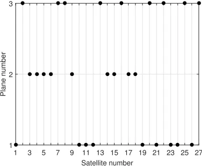
The constellation considered in this study is a Walker Delta 56◦:27/3/1 constellation in MEO.1 _{In the}

notationi:t/p/f used to describe Walker Delta constellation,irepresents the inclination of the orbit,tthe total number of satellites,pthe number of planes andf is the relative spacing between satellites in adjacent planes. The semimajor axis of the orbits isaM EO= 24200 km and the right ascension of the ascending node of the three planes are equally spaced of 120 deg. It is assumed that the only perturbation acting on the satellites is due to the second order zonal harmonic of the geopotential, J2. This perturbation causes the right ascension of the orbital plane to drift at a rate given by:2

˙ Ω =−3

2nJ2

R⊕

aM EO 2

cosiM EO (1)

where n = pµ/a3

M EO is the mean motion of the satellite on its orbit, µ is the Earth’s gravitational parameter,R⊕ is the Earth radius andJ2= 1.0826·10−2 andiM EO= 56 deg.

A graphical representation of the considered constellation is given in Figure 1, where the axis are in Earth- radii.

III.

Deployment Sequence

In this section the method adopted to define the deployment sequence is described. The deployment sequence allows to define which satellite is allocated to which slot and the order with which these slots should be filled.

3 2 1 0 x [R

⊕]

-1 -2 -3 -2 0 x [R

⊕]

2 -1

0 1 2 3

-2 -3

x [R

⊕

]

Figure 1. Walker Delta 56◦:27/3/1 constellation.

caps, the problem was tackled using an analogy: each satellite was considered an electrically charged particle that could be collocated in one of the available slots. By using this analogy, the desired coverage strategy translates into the strategy that minimises of the integral over time of the energy of the whole system, assuming that the time interval between the collocation of each subsequent satellite is constant.

A brute force analysis of all the possibilities for 27 satellites would require considering 27! combinations (≈ 1028_{), so in order to solve the problem a greedy tree-search approach was used instead. With this approach,}

an initial position for the first satellite was chosen. Then, the integral over time of the energy resulting from the addition of one satellite was computed for all possible remaining positions, and all combinations with the same minimum were stored. With this approach, at each stage, a locally optimal choice is made, in an attempt to find the global optimum. This was repeated, stage by stage, for all promising combinations until all the satellites were collocated, and was also repeated for every possible choice for the initial satellite. This greedy approach does not guarantees to find the global optimal solution but provides good solutions in a reasonable amount of time. Due to the symmetries present in the problem, multiple equivalent optimal solutions are possible, but only one is considered in the following.

The optimal satellite deployment sequence obtained is shown in Figure 2, where the x axis indicates the number of the satellite and the y axis the plane (from 1 to 3) of arrival of the satellite.

Satellite number

1 3 5 7 9 11 13 15 17 19 21 23 25 27

Plane number

1 2 3

IV.

Launchers

In this study two European launchers are considered: Vega3 _{and Ariane 5.}4 _{For each launcher, models}

relating payload mass, target inclination and semimajor axis are developed from available data as simple second order bivariate polynomials. Figures 3 and 4 show the resulting surface for the two launchers.

Figure 3. Relationship between mass and injection semimajor axis and inclination for Vega

Figure 4. Relationship between mass and injection semimajor axis and inclination for Ariane

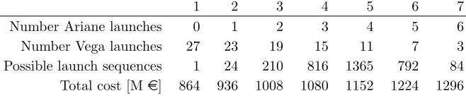
Due to fairing limitations, it is assumed that Vega can carry one satellite in orbit, while Ariane can carry four satellites of the constellation. With this assumption, and for a constellation of 27 satellites, 7 possible combinations of Ariane and Vega launches allow the deployment of the entire constellation. The total cost of the launches differ for the seven possibilities. Assuming a cost per launch of 32 million euros for Vega and 200 million euros for Ariane, the total cost reported in Table 1 can be obtained. The table also reports, for each combination, the total number of possible launch sequences.

Table 1. Combinations, launch sequences and total cost of Vega and Ariane launches for the deployment of a constellation of 27 satellites

1 2 3 4 5 6 7

Number Ariane launches 0 1 2 3 4 5 6

Number Vega launches 27 23 19 15 11 7 3

Possible launch sequences 1 24 210 816 1365 792 84 Total cost [Me] 864 936 1008 1080 1152 1224 1296

Table 1 shows that two limit value exist for the cost of the launches. The minimum cost is obtained when all the launches are realised using Vega (option 1). The maximum cost is obtained when 6 launches are realised with Ariane and 3 with Vega (option 7). Assuming a rate of one launch per year, option 1 would require 27 years while option 7 would require 9 years, so there is a clear trade-off between total cost of the launches and total deployment time (which relates to a reduced pay-off). Due to the very large total number of possible launch sequences for the 7 deployment strategies (each of which would be followed by the solution of a bi-objective optimisation problem for the minimisation of the ∆V and the maximisation of pay-off), only a systematic study of the two limit cases was performed in the rest of the study.

V.

Low-Thrust Transfer

the injection to the final orbit.

Once the launchers leaves the satellite on the injection orbit, the low-thrust engine is operated to obtain the following variation of the orbital elements:

• ainj→aM EO=ainj+ ∆a

• iinj→iM EO=iinj+ ∆i

• Ωinj→ΩM EO= Ωinj+ ∆Ω

Four possible low-thrust strategies are considered to achieve these variations, simultaneously, in a given time of flightT oF. These strategies are presented in the following subsections.

A. Strategy 1: ∆ΩJ2 + (∆a,∆i)

In this case the transfer from injection to operational orbit is realised in two phases:

1. During the first phase the spacecraft waits on its initial injection orbit, where the effects of the drift of Ω due to J2 is higher (Equation 1). The low-thrust engine is off during this phase and the variation of aandiis zero. The time of flight associated to this phase is identified asT oF1S1. The right ascension

at the end of this phase is identified as ΩS1

1f. The variation in time of Ω is:

˙ Ω =−3

2 √

µJ2R2⊕cosiinja−

7/2

inj (2)

so thatT oFS1

1 and ΩS1f1 are linked by the following relationship:

T oF₁S1= Ω S1 1f −Ωinj

3 2

√

µJ2R⊕2 cosiinja

−7/2

inj

(3)

2. The second phase is realised switching on the low-thrust engine, during two thrust arcs per revolution. During this phase the semimajor axis and inclination change from their initial value to their final values. The variable drift due to J2 is such that at the end of the transfer the right ascension changes from ΩS1

1f to ΩM EO. The time of flight of the second phase isT oF2S1. The simultaneous variation ofa

andiin a given time of flightT oF2S1can be obtained with two tangential thrust arcs of semi-amplitude

αand elevation angleβ, centered at the nodal points of the orbit. β has equal and opposite value on the two thrust arcs. The relevant equations for this transfer can be obtained from the Gauss equations for the variation in time of the semimajor axis and inclination of circular orbits with tangential thrust:5

da dt =

2a2

h fcosβ di

dt =f a

hcosusinβ

(4)

wherehis the angular momentum of the orbit,f is the low-thrust acceleration anduis the argument of the latitude.

The variation of aandiwith the argument of the latitudeuof can be expressed as:

da du = da dt dt du = 2a3

µ fcosβ di du = di dt dt du =

f a2_sinβcosu

µ

(5)

The mean variation of aover one orbital revolution can be obtained from:

¯ _da dt = 1 T Z α −α da du+

Z π+α

π−α da du

to obtain:

di dt =

2f asinβsinα

π√µa (7)

Analogously, for the inclination:

di dt =

2f asinβsinα

π√µa (8)

In order for aand ito reach the final value simultaneously, the following equation is integrated from ainj toaM EO and from iinj toiM EO:

da di =

2aαcosβ

sinαsinβ (9)

This results in:

tanβ= 2α(iM EO−iinj) sinαlog(aM EO/ainj)

(10)

The time of flight of the transfer can be expressed as a function of αand the initial and final orbital elements as:

T oF₂S1= π 2f α

r _µ

ainj −

r _µ

aM EO

s

1 + 4α

2_(i

M EO−iinj)

2

sin2αlog2(aM EO/ainj)

(11)

By using the equation above it is possible to findαand thereforeβ that allow to realise a variation of aandiin a given time of flight. The cost of the transfer can be computed analytically from:

∆V = 1 cosβ

r _µ

ainj −

r _µ

aM EO

(12)

During the variation ofaandithe right ascension changes due to J2 and the variation ofaandiwith time. The value of Ω at the end of the second phase can be expressed as:

ΩS_2f1= ΩS_1f1+ k1 1 +k2

2

k3 (13)

where

k1=−

3πµJ2R2

4a4

injfsinβsinα exp

_{4 log(a}

M EO/ainj)iinj (iM EO−iinj)

k2=

4 log(aM EO/ainj) (iM EO−iinj)

k3= exp(k2iM EO)(k2cosiM EO+ siniM EO)−exp(k2iinj)(k2cosiinj+ siniinj)

(14)

If the combined transfer ∆ΩJ2 + (∆a,∆i) has to be realised in a total time of flightT oFtot, the values ofT oF1S1andT oF2S1 can be computed solving the system of equations given by ΩS2f1= ΩM EO and:

T oF₁S1+T oF₁S2=T oFtot (15)

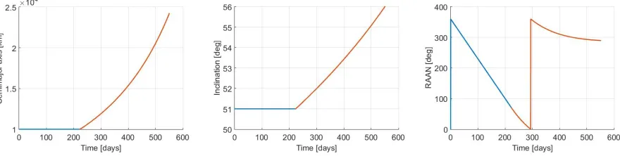
and using Equations 3 and 13. The possibility of realising the transfer by applying first (∆a,∆i) and then ∆ΩJ2 is not considered since the variation of Ω with J2 at high values of a, such as aM EO, is limited (Equation 1). Figure 5 shows an example of transfer realised using this strategy, with time of flight of 550 days and low-thrust acceleration equal to 1.205·10−4_m/s2_{. The variation of semimajor axis is from 10000}

to 24200 km, the inclination changes from 51 to 56 deg and the right ascension changes from 0 deg to 150 deg. The relevant parameter of the low-thrust control areα= 49.13 deg andβ= 12.62 deg. The cost of the transfer is ∆V = 2.31 km/s.

Figure 5. Variation ofa,iand Ωduring low-thrust transfer with strategy 1.

B. Strategy 2: (∆a,∆i) + ∆Ωβ

In the second considered low-thrust strategy the transfer from injection to operational orbit is realised in two phases:

1. During the first phase aandi are changed from their initial values ainj and iinj to their final values in MEO using the same method used in phase 2 of Strategy 1, with low-thrust applied on two thrust arcs of semi-amplitudeα1. This variation takes place in a time of flightT oF1S2. The right ascension

at the end of the first phase is computed from Equation 13 as:

ΩS_1f2= Ωinj+ k1

1 +k2 2

k3 (16)

2. During the second phase Ω is changed using the low-thrust engine and out-of-plane thrust, with two thrust arcs of semi-amplitude α2 and elevation angle β = 90 deg applied at the apsidal points of the

orbit.

Using the Gauss equation for Ω, the variation of Ω with time is given by:

dΩ dt =f

asinusinβ

hsini (17)

The corresponding variation of Ω with the argument of the latitude is:

dΩ du =

f a2_sinu

sini (18)

The mean variation of Ω during one orbital revolution, due to both the out-of-plane thrust and J2, is:

dΩ dt =

2fsinα2

πsini

r

µ a −

3 2

√

µJ2R2⊕cosia−

If the variation of Ω has to be realised in a time of flightT oF2S2, the semi-amplitude of the thrust arcs

can be computed from:

sinα2=

ΩM EO−ΩS21f T oFS2

2

+3₂√µJ2R2⊕cosiM EOa

−7/2

M EO

2f πsiniM EO

q _µ

aM EO

(20)

The cost associated to the variation of Ω can be computed analytically from:

∆V = siniM EO

r _µ

aM EO α

sinα(ΩM EO−Ω S2

1f) (21)

When the combined transfer (∆a,∆i) + ∆Ωβ has to be realised in a total time of flight T oFtot, the equations defined above, together with T oF1S1+T oF1S2 = T oFtot, do not provide a sufficient number of equations to solve the system and to find α1 and α2. It is possible however to define different arbitrary

values ofT oF1S2< T oFtot and compute the corresponding values ofα1, α2 andT oF2S2. In particular, it is

possible to find aT oFS1

1 such that the ∆V of the transfer is the minimum possible value.

The possibility of realising the transfer by applying first ∆Ωβ and then (∆a,∆i) is not considered since the variation of Ω with J2 at low altitude is higher than the variation of Ω obtainable with the low-thrust engine.

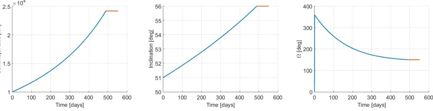
An example of transfer realised with this strategy is shown in Figure 6. The initial and final orbital elements are those used for the previous example . The transfer is realised with ∆V = 2.3045 km/s and the parameter of the low-thrust control areα1= 32.70 deg,β = 11.78 deg and α2 = 21.77 deg.

Figure 6. Variation ofa,iand Ωduring low-thrust transfer with strategy 2.

C. Strategy 3: (∆a,∆Ω)N oW ait + ∆i

The low-thrust transfer using strategy 3 is realised in two phases:

1. During the first phase a tangential thrust withβ= 0 is used to increase the semimajor axis fromainj to aM EO. The engine is on during two thrust arcs per revolution, of semi-amplitudeα1.

The time of flight is given by:

T oF₁S1= π 2f α1

r _µ

ainj −

r _µ

aM EO

(22)

The cost of this phase can be computed analytically from:

∆V =

r _µ

ainj −

r _µ

aM EO

The right ascension at the end of the transfer can be obtained by integratingdΩ/daobtained from the equations fordΩ/dtandda/dt. This results in:

ΩS_1f3= Ωinj+ 3 32

µJ2R2⊕cosiinj f α1

1 a4

M EO

− 1

a4

inj !

(24)

2. During the second phase the thrust is applied during two thrust arcs per revolution, of semi-amplitude α2, with elevationβ = 90 deg, to change the inclination fromiinj toiM EO.

The time required can be computed from:

T oF2S2=

iM EO−iinj

2f π

pµ asinα2

(25)

The cost of this phase is:

∆V = α2 sinα2

r _µ

aM EO

(iM EO−iinj) (26)

The variation of right ascension during this phase can be obtained from Equation 13 and subsection A, as particular case in which the variation of semimajor axis is zero:

ΩS2f3= ΩS1f3+ 3 4

πµJ2R2⊕

f a4

M EOsinα2

(siniinj−siniM EO) (27)

The above equations can be used to solve the problem in which the entire transfer has to be realised in a given time of flight. In particular the equations to satisfy are:

T oF₁S3+T oF₂S3=T oFtot

ΩS2f3= ΩM EO

(28)

The possibility of realising the transfer by applying first ∆iand then (∆a,∆Ω) is not considered since the cost of the variation ofiat low altitude is higher.

An example of transfer realised with this strategy is shown in Figure 7. The transfer is realised with ∆V = 2.6201 km/s,α1= 33.68 deg andα2 = 30.31 deg.

Figure 7. Variation ofa,iand Ωduring low-thrust transfer with strategy 3.

D. Strategy 4: (∆a,∆Ω)W ait + ∆i

This strategy is analogous to strategy 3 presented above. The difference is in the introduction of a waiting timeTS4

wait, during phase 1, when the engine is off and the drift of Ω due to J2 can be exploited. The first of Equations 28 is modified as:

and Equation 27 is now expressed as:

ΩS_1f4= Ωinj+ 3 32

µJ2R2⊕cosiinj f α1

1 a4

M EO

− 1

a4

inj !

−ΩT˙ _waitS4 (30)

In this case, as for strategy 2, the number of relevant equations is not sufficient to solve the problem when the transfer has to be realised in a total time of flightT oFtot. A value ofT oF1S4< T oFtot exist however for which the ∆V of the transfer is minimum.

An example of transfer realised with this strategy is shown in Figure 8. The blue lines represent the waiting time on the initial orbit. The transfer is realised with ∆V = 2.6104 km/s andα1= 85.81 deg and

α2= 8.22 deg.

Figure 8. Variation ofa,iand Ωduring low-thrust transfer with strategy 4.

E. Low-thrust strategies comparison

Figure 9 shows the ∆V required to realise the transfer defined in the previous example, for different values of the times of flight and using the four strategies defined in the previous subsection. For strategies 2 and 4, where a unique solution does not exist, the plotted solutions are the ones corresponding to the values of T oF1andT oF2 providing the lower value of the ∆V for that transfer.

For the multi-objective optimisation of constellation deployment strategy 1 is considered. This gives lower ∆V than strategy 3 and 4 and, compared to strategy 2, does not require out-of-plane maneuvers to change the right ascension of the ascending node.

The discontinuity in the curve relative to strategy 1 atT oF of approximately 600 days is due to a jump of the variation of Ω, during the first phase, from less than 2πto a variation of more than 2π, that is a jump from|ΩS1

1f−Ωinj|<2πto|ΩS1f1−Ωinj|>2π. This causes the time of flight available for the second phase to be reduced of an amount equal to 2π/Ω, thus increasing the total ∆V˙ . It has to be noted that a variation of more than 2πduring the first phase of strategy 1 might be necessary in order to reach simultaneously the final orbital elements at the end of the transfer.

VI.

Multi-Objective Deployment Optimisation

The objectives of the optimisation of the constellation deployment are the minimisation of the maximum ∆V of all the low-thrust transfer, the maximisation of the profit of the constellation and the minimisation of the cost of the launches. As regards the cost of the launches, the two extreme cases in Table 1 are considered. The objectives considered in the following are therefore:

• Minimisation of the maximum ∆V of the low-thrust transfers

• Maximisation of the profit obtained from the deployment of the constellation. Each satellite is assumed to generate profit from the moment it reaches its final orbit, up to an an end date defined as 5 years after the last launch. The adimensional profit rate considered in this work is of one unit per day.

Figure 9. ∆V of the low-thrust transfer for different time of flights and low-thrust strategies.

agents or simply collect information on a neighborhood of each agent. In MACS2 the idea of search di-rections was introduced in the logic of the agents, which could select new candidate solutions according to either dominance or Tchebycheff scalarisation. All solutions that are non-dominated or satisfy Tchebycheff scalarisation criterion are stored in a global archive that contains the best approximation of the Pareto front. Therefore, at each iteration of MACS2, archive maintains the set of locally Pareto optimal solutions, while the populations of agents explore the parameter space in search for improvements. MACS2 was shown to be very effective compared to more traditional multi-objective optimisers at providing a good balance of convergence and spreading of the solutions.

The vector of optimisable parameters, that is handled by MACS2, includes, for each satellite launched:

• Semimajor axis of the injection orbit,ainj

• Inclination of the injection orbit,iinj

• Right ascension of the ascending node of the injection orbit, Ωinj

• Time of flight from the injection to the operational orbit,T oF

When four satellites are launched with Ariane, the time of flights of the four satellites are constrained such that the sequence of deployment defined in Section III is still satisfied. The final semimajor axis and inclination of the arrival orbit are aM EO and iM EO. The right ascension of the arrival orbits is computed from Equation 1, based on the arrival time of the satellite on the selected orbit. The boundaries for the parameters to optimise are:

6878 km≤ainj≤9378 km

0 deg≤iinj≤50 deg

0 deg≤Ωinj≤ 360 deg

300 days≤T oF ≤1500 days

(31)

The selected values of admissible ainj have been chosen in order to avoid regions where the effect of the drag is not negligible (a <6878 km) and regions where the drift of Ω due toJ2 is not very significant

(a >9378 km). Likewise the range of inclinations is restricted to exploit natural dynamics for the change of Ω.

The considered value of the acceleration for the low-thrust transfer is 1.20510−4_m/s2_.

VII.

Results

A. Maximum launch cost with minimum launch time

Option 7 in Table 1 identifies the solution with minimum launch times (9 years, in the assumption of 1 launch per year) but maximum cost for the launches (1296 million euros). The total cost of the 9 launches is fixed but different combinations of sequences of Ariane and Vega launches exist for that cost. In particular, 84 possible combinations of launches can be identified; some of these combinations are presented in Table 2, where V stands for launch with Vega and A for launch with Ariane.

Table 2. Possible combinations of Ariane and Vega launches for solution with deployment of the constellation in 9 launches

XX XX

XX

XX_X

X

Comb.

Launch

1 2 3 4 5 6 7 8 9

1 V V V A A A A A A

2 V V A V A A A A A

.. .

78 A A A A V A V V A

.. .

81 A A A A A V V V A

82 A A A A A V V A V

83 A A A A A V A V V

84 A A A A A A V V V

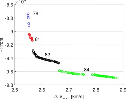
Each combination defined in Table 2 generates a Pareto set in the plane ∆Vmax-Profit. The 84 Pareto sets obtained are shown in Figure 10, with different color for each combination. A single Pareto set can be obtained by considering the non-dominated solution of the 84 combinations. This is shown in Figure 11, along with a number identifying the sequence of Vega and Ariane launchers (Table 2).

∆ V_max [km/s]

2.4 2.6 2.8 3 3.2 3.4

- Profit

×104

-10 -9.5 -9 -8.5 -8 -7.5

Figure 10. Pareto sets of the 84 combinations of

launches corresponding to option 7 in Table 1.

∆ V_max [km/s]

2.5 2.6 2.7 2.8 2.9

- Profit

×104

-9.8 -9.6 -9.4 -9.2 -9 -8.8 -8.6

78

81

82

84

Figure 11. Non-dominated solutions resulting from the combinations of the 84 Pareto sets in Figure 10

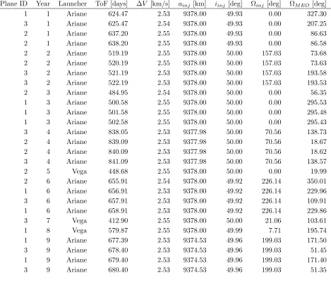
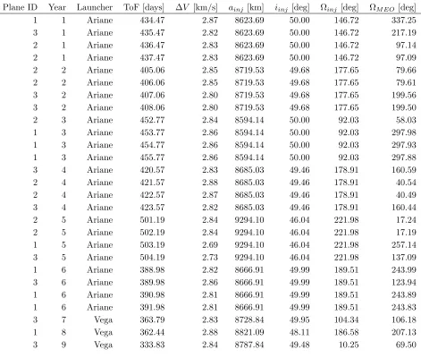
Results in Figure 11 show that only four combinations of launches give non-dominated results. These are combinations 78, 81, 82 and 84. The sequence of launchers for these four cases can be found in Table 2. The solutions of combination 84 are characterised by higher profit and higher maximum ∆V while the solutions of combination 78 are characterised by lower profit and lower maximum ∆V.

the right ascension of the final orbit.

The times of flight in Table 3 are averagely higher than the times of flight in Table 4. Higher times of flight results in lower ∆V but also lower pay-off from the constellation, since the final time of full disposal of the constellation is shifted in time.

The optimal injection orbits are in both cases characterised by a value of the inclinationiinj close to the upper limit of 50 deg. This is due to the fact that changes of inclination are expensive in term of ∆V and require long times of flight and are therefore penalised both in term of ∆Vmax and profit.

Table 3. Solution with minimum maximum∆V and lower profit (combination of launches 78)

Plane ID Year Launcher ToF [days] ∆V [km/s] ainj [km] iinj [deg] Ωinj [deg] ΩM EO [deg]

1 1 Ariane 624.47 2.53 9378.00 49.93 0.00 327.30

3 1 Ariane 625.47 2.54 9378.00 49.93 0.00 207.25

2 1 Ariane 637.20 2.55 9378.00 49.93 0.00 86.63

2 1 Ariane 638.20 2.55 9378.00 49.93 0.00 86.58

2 2 Ariane 519.19 2.55 9378.00 50.00 157.03 73.68

2 2 Ariane 520.19 2.55 9378.00 50.00 157.03 73.63

3 2 Ariane 521.19 2.53 9378.00 50.00 157.03 193.58

3 2 Ariane 522.19 2.53 9378.00 50.00 157.03 193.53

2 3 Ariane 484.95 2.54 9378.00 50.00 0.00 56.35

1 3 Ariane 500.58 2.55 9378.00 50.00 0.00 295.53

1 3 Ariane 501.58 2.55 9378.00 50.00 0.00 295.48

1 3 Ariane 502.58 2.55 9378.00 50.00 0.00 295.43

3 4 Ariane 838.05 2.53 9377.98 50.00 70.56 138.73

2 4 Ariane 839.09 2.53 9377.98 50.00 70.56 18.67

2 4 Ariane 840.09 2.53 9377.98 50.00 70.56 18.62

3 4 Ariane 841.09 2.53 9377.98 50.00 70.56 138.57

2 5 Vega 448.68 2.55 9378.00 50.00 0.00 19.99

2 6 Ariane 655.91 2.54 9378.00 49.92 226.14 350.01

1 6 Ariane 656.91 2.53 9378.00 49.92 226.14 229.96

3 6 Ariane 657.91 2.53 9378.00 49.92 226.14 109.91

1 6 Ariane 658.91 2.53 9378.00 49.92 226.14 229.86

3 7 Vega 412.90 2.55 9378.00 50.00 21.06 103.61

1 8 Vega 579.87 2.55 9378.00 49.99 7.71 195.74

1 9 Ariane 677.39 2.53 9374.53 49.96 199.03 171.50

3 9 Ariane 678.40 2.53 9374.53 49.96 199.03 51.45

1 9 Ariane 679.40 2.53 9374.53 49.96 199.03 171.40

3 9 Ariane 680.40 2.53 9374.53 49.96 199.03 51.35

B. Minimum launch cost with maximum launch time

Option 1 in Table 1 identifies the solution with maximum launch times (27 years, under the assumption of 1 launch per year) but minimum total cost for the launches (864 million euros).

In this case only one combination exist for the 27 launches with Vega. The resulting Pareto front is shown in Figure 12.

Table 4. Solution with higher maximum∆V and higher profit (combination of launches 84)

Plane ID Year Launcher ToF [days] ∆V [km/s] ainj [km] iinj [deg] Ωinj [deg] ΩM EO [deg]

1 1 Ariane 434.47 2.87 8623.69 50.00 146.72 337.25

3 1 Ariane 435.47 2.82 8623.69 50.00 146.72 217.19

2 1 Ariane 436.47 2.83 8623.69 50.00 146.72 97.14

2 1 Ariane 437.47 2.83 8623.69 50.00 146.72 97.09

2 2 Ariane 405.06 2.85 8719.53 49.68 177.65 79.66

2 2 Ariane 406.06 2.85 8719.53 49.68 177.65 79.61

3 2 Ariane 407.06 2.80 8719.53 49.68 177.65 199.56

3 2 Ariane 408.06 2.80 8719.53 49.68 177.65 199.50

2 3 Ariane 452.77 2.84 8594.14 50.00 92.03 58.03

1 3 Ariane 453.77 2.86 8594.14 50.00 92.03 297.98

1 3 Ariane 454.77 2.86 8594.14 50.00 92.03 297.93

1 3 Ariane 455.77 2.86 8594.14 50.00 92.03 297.88

3 4 Ariane 420.57 2.83 8685.03 49.46 178.91 160.59

2 4 Ariane 421.57 2.88 8685.03 49.46 178.91 40.54

2 4 Ariane 422.57 2.87 8685.03 49.46 178.91 40.49

3 4 Ariane 423.57 2.82 8685.03 49.46 178.91 160.44

2 5 Ariane 501.19 2.84 9294.10 46.04 221.98 17.24

2 5 Ariane 502.19 2.84 9294.10 46.04 221.98 17.19

1 5 Ariane 503.19 2.69 9294.10 46.04 221.98 257.14

3 5 Ariane 504.19 2.73 9294.10 46.04 221.98 137.09

1 6 Ariane 388.98 2.82 8666.91 49.99 189.51 243.99

3 6 Ariane 389.98 2.86 8666.91 49.99 189.51 123.94

1 6 Ariane 390.98 2.81 8666.91 49.99 189.51 243.89

1 6 Ariane 391.98 2.81 8666.91 49.99 189.51 243.83

3 7 Vega 363.79 2.83 8728.84 49.95 104.34 106.18

1 8 Vega 362.44 2.88 8821.09 48.11 186.58 207.13

3 9 Vega 333.83 2.84 8787.84 49.48 10.25 69.50

The higher values of ∆V are due to the limited launch capabilities of Vega with respect to Ariane. The inclination of the injection orbit is indeed lower than in Table 3 and 4.

VIII.

Conclusions

∆ V

max [km/s]

4.2 4.4 4.6 4.8 5 5.2 5.4

- Profit

×105

-1.74 -1.73 -1.72 -1.71 -1.7 -1.69

Figure 12. Pareto set corresponding to option 1 in Table 1.

cost was also studied. In this case the sequence of launches is fixed and only one Pareto set exists.

Future study will consider the possibility of realising the low-thrust transfer with an out-of-plane manuever to change the right ascension of the orbit and will extend the study to all the possible range of costs of the launches options.

Acknowledgments

This research was partially funded by Airbus Defence and Space and partially by the ESA NPI pro-gramme. The authors would like to thank Mr Stephen Kemble, at Airbus DS, for his support and advice. The authors would like to thank the Institute of Engineering and Technology for the IET Travel Award to attend the Space 2016 Forum and present this work.

References

1_{Fortescue, P., Stark, J., Swinerd, G., Spacecraft System Engineering, Wiley, 2011}

2_{Vallado, D., Fundamentals of Astrodynamics and Applications, Space Technology Library, 2007}

3_{http://www.arianespace.com/wp-content/uploads/2015/09/Vega-Users-Manual Issue-04 April-2014.pdf, Accessed May}

2016.

4_{http://www.arianespace.com/wp-content/uploads/2015/09/Ariane5 users manual Issue5 July2011.pdf, Accessed May}

2016.

5_{Battin, R. H, An introduction to the mathematics and methods of astrodynamics, AIAA, 1999.}

6_{Ricciardi, L., Vasile, M., Improved archiving and search strategies for Multi Agent Collaborative Search, International}

Table 5. Solution with higher maximum∆V and higher profit for launches with Vega only

Plane ID Year Launcher ToF [days] ∆V [km/s] ainj [km] iinj [deg] Ωinj [deg] ΩM EO [deg]

1 1 Vega 479.96 4.10 8056.69 35.19 202.69 334.87

3 2 Vega 538.48 5.10 7674.50 27.23 158.37 192.67

2 3 Vega 434.60 4.21 7922.37 35.85 196.60 58.99

2 4 Vega 534.96 4.49 8091.04 33.18 118.76 34.60

2 5 Vega 461.75 3.75 8338.37 38.84 245.55 19.31

2 6 Vega 623.39 4.79 8101.14 26.79 149.88 351.72

3 7 Vega 618.04 4.95 8154.60 26.34 254.89 92.87

3 8 Vega 592.09 5.16 8139.59 26.36 190.83 75.10

2 9 Vega 551.55 4.65 8116.09 28.58 247.00 298.09

1 10 Vega 562.23 4.84 7893.93 28.91 244.28 158.41

1 11 Vega 505.64 4.95 7458.27 30.74 141.15 142.24

1 12 Vega 385.42 3.59 7822.33 42.63 173.26 129.41

3 13 Vega 515.57 4.81 8554.87 28.90 192.58 343.47

2 14 Vega 462.22 4.01 8039.53 37.85 121.40 207.13

2 15 Vega 509.53 4.88 8045.47 29.79 103.71 185.53

3 16 Vega 556.41 4.12 8920.56 29.71 106.02 283.95

2 17 Vega 573.93 4.95 8221.12 26.17 127.12 143.90

2 18 Vega 576.23 4.85 8092.05 28.47 224.02 124.65

1 19 Vega 471.27 4.57 8154.85 32.28 176.69 351.02

3 20 Vega 550.67 4.70 8592.51 29.14 156.64 207.74

1 21 Vega 551.40 4.94 8370.21 25.38 160.31 308.57

3 22 Vega 639.89 4.83 8471.34 24.20 208.49 164.81

1 23 Vega 573.90 4.95 7973.60 25.48 207.63 269.14

1 24 Vega 508.33 4.31 8094.43 32.24 134.14 253.44

3 25 Vega 609.78 5.36 8417.44 22.98 132.38 109.00

1 26 Vega 557.36 4.83 8334.08 28.74 221.32 212.62