Copula regression spline models for binary outcomes

      

City, University of London Institutional Repository

Citation

:

Radice, R. ORCID: 0000-0002-6316-3961, Marra, G. and Wojtys, M. (2016). Copula regression spline models for binary outcomes. Statistics and Computing, 26(5), pp. 981-995. doi: 10.1007/s11222-015-9581-6

This is the accepted version of the paper.

This version of the publication may differ from the final published

version.

Permanent repository link: http://openaccess.city.ac.uk/20927/

Link to published version

:

http://dx.doi.org/10.1007/s11222-015-9581-6

Copyright and reuse:

City Research Online aims to make research

outputs of City, University of London available to a wider audience.

Copyright and Moral Rights remain with the author(s) and/or copyright

holders. URLs from City Research Online may be freely distributed and

linked to.

Copula regression spline models for binary outcomes

Rosalba Radice

∗

Department of Economics, Mathematics and Statistics

Birkbeck, London, U.K.

Malet Street, London WC1E 7HX, U.K.

Giampiero Marra

Department of Statistical Science

University College London

Gower Street, London WC1E 6BT, U.K.

Małgorzata Wojty´s

School of Computing and Mathematics

University of Plymouth

Drake Circus, Plymouth PL4 8AA, U.K.

Abstract

We introduce a framework for estimating the effect that a binary treatment has on a binary

outcome in the presence of unobserved confounding. The methodology is applied to a case

study which uses data from the Medical Expenditure Panel Survey and whose aim is to

esti-mate the effect of private health insurance on health care utilization. Unobserved confounding

arises when variables which are associated with both treatment and outcome are not

avail-able (in economics this issue is known as endogeneity). Also, treatment and outcome may

exhibit a dependence which cannot be modeled using a linear measure of association, and

observed confounders may have a non-linear impact on the treatment and outcome variables.

The problem of unobserved confounding is addressed using a two-equation structural latent

variable framework, where one equation essentially describes a binary outcome as a function

of a binary treatment whereas the other equation determines whether the treatment is received.

Non-linear dependence between treatment and outcome is dealt with by using copula

func-tions, whereas covariate-response relationships are flexibly modeled using a spline approach.

Related model fitting and inferential procedures are developed, and asymptotic arguments

presented.

Key Words: Bivariate binary outcomes; Copula; Endogeneity; Penalized regression spline;

Simultaneous equation estimation; Unobserved confounding.

1

Introduction

Quantifying the effect of a non-randomly assigned treatment on an outcome is a challenging task in observational studies. An approach to calculate such an effect is to match subjects on the

basis of observed features or the so-called propensity score, and then compute the treatment effect

as the difference between the observed responses of the matched subjects corresponding to the

levels of the treatment (e.g., Heckman et al., 1997; Rosenbaum & Rubin, 1983). However, this

method is only valid when the unobserved variables that influence the treatment are independent

of the outcome, conditional on the covariates in the model. We consider the situation in which the

researcher is interested in estimating the effect of a binary treatment on a binary outcome in the

presence of unobserved confounders (i.e., unknown or not readily quantifiable variables associated

with both treatment and outcome). In economics, this problem is commonly framed in terms of

a regression model from which important regressors have been omitted and hence become a part

of the model’s error term. In this context, the treatment is termed exogenous if it is not associated with the error term after conditioning on the observed confounders, and endogenous otherwise. We

address this issue by specifying a simultaneous model for treatment and outcome; this route has

been previously taken by several scholars (e.g., Chib & Hamilton, 2002; Greene, 2012; Heckman,

1978; Maddala, 1983; Marra & Radice, 2011a). Other approaches are available to account for

unobserved confounding; see the detailed review of Clarke & Windmeijer (2012).

To fix ideas, let us consider a case study which uses data from the Medical Expenditure Panel

Survey (MEPS) and whose goal is to estimate the effect of having private health insurance on

the probability of using health care services. Private health insurance status, which is an important

determinant of the use of health care services, is a potentially endogenous variable. This is because unobserved variables, such as allergy and risk aversiveness, are likely to influence both health

service utilization and private insurance decision. Sometimes the effect of private health insurance

can be interpreted as adverse selection or moral hazard (e.g., Buchmueller et al., 2005). Adverse

selection occurs when individuals with a greater demand for medical care, because of poor health

for instance, are expected to have a greater demand for insurance. Moral hazard refers to the

tendency of people to be more inclined to seek health services, and doctors to be more inclined

to refer them when all costs are covered. The matter is further complicated by the fact that the

effects of observed confounders, such as age and education, may be complex since they embody

productivity and life-cycle effects that are likely to influence private health insurance and health care utilization non-linearly. If these relationships are mismodeled then the effect of insurance

on the probability of using health care services may be biased (e.g., Marra & Radice, 2011a).

Moreover, insurance status and health care utilization may exhibit a non-Gaussian association

(Winkelmann, 2012).

Unobserved confounding can be controlled for by using the recursive bivariate probit model

(Heckman, 1978). This model controls for unobserved confounding by using a two-equation

struc-tural latent variable framework, where one equation essentially describes a binary outcome (e.g.,

health care utilization) as a function of a binary treatment (e.g., insurance coverage) whereas the

other equation determines whether the treatment is received. The model is completed by assum-ing that the latent errors of the two equations follow a standard bivariate Gaussian distribution

with correlationθ;θ ₆= 0suggests that unobserved confounding is present, hence joint estimation

of the two equations is required. Some applications in economics and bio-statistics are provided

(2009) and Li & Jensen (2011). The limitations of this model are, however, the inability to deal

ef-fectively with non-linear covariate effects and non-Gaussian dependencies between the treatment

and outcome equations. To model flexibly covariate-response relationships, Chib & Greenberg

(2007) and Marra & Radice (2011a) introduced Bayesian and likelihood estimation methods based

on penalized splines, respectively. To deal with the problem of non-Gaussian dependence between

treatment and outcome, Winkelmann (2012) discussed a modification of the recursive bivariate

probit that maintains the Gaussian assumption for the marginal distributions of the two equations

while introducing non-Gaussian dependence between them using the Frank and Clayton copulas.

The contribution of this article is twofold, one methodological and the other practical. First, we extend the procedures discussed in Marra & Radice (2011a) and Winkelmann (2012) to make

it possible to deal simultaneously with unobserved confounding, non-linear covariate effects and

non-Gaussian dependencies between treatment and outcome. In particular, we generalize the

pe-nalized likelihood estimation approach based on the assumption of bivariate normality presented

in Marra & Radice (2011a) by allowing for non-Gaussian dependencies between the two model

equations; this is achieved by employing some classic copulas, such as Clayton, Frank, Gumbel

and Joe, and the rotated versions of Clayton, Gumbel and Joe. We also provide some theoretical

ar-gumentation related to the asymptotic behavior of the proposed estimator and the ensuing formula

to calculate the treatment effect. Second, we implement the methods discussed in this article in theRpackageSemiParBIVProbit(Marra & Radice, 2015). This can be particularly attractive

to practitioners who wish to fit such models. Swihart et al. (2014) and Genest et al. (2013) have

also adopted the copula paradigm to model multiple binary outcomes. One of the main

contribu-tions of the former article is to establish the connection between existing marginalized multilevel

models and copulas. The work by Genest et al. (2013) discusses models for vectors of binary

out-comes in the which the marginal distributions depend on covariates through logistic regressions

and the dependence structure is modeled through meta-elliptical copulas. Our approach does not

deal with multivariate binary outcomes, although it can be extended to this context. However, as

opposed to Swihart et al. (2014) and Genest et al. (2013), the proposed methodology can account for non-linear covariate effects, and more importantly can mitigate the issue of endogeneity.

The rest of the paper is organized as follows. Section 2 mainly discusses the model structure,

parameter estimation, confidence intervals and variable selection. Section 3 applies the proposed

methodology to the MEPS data mentioned above, whereas Section 4 discusses the limitations of

the proposed framework and concludes with some future extensions. The online supplementary

material includes some of the details required to calculate the asymptotic variance of the

treat-ment effect, details on the structure of the score vector and Hessian matrix used in the algorithm,

asymptotic considerations related to the proposed estimator and the ensuing formula to calculate

2

Methods

2.1

Model definition

The focus is on a pair of random variables(y1i, y2i), fori = 1, . . . , n, whereyvi ∈ {0,1}, v can

take values 1 and 2, and n represents the sample size. Variable y1i refers to the treatment and

y2i to the outcome. The observed yvi is determined by a latent continuous variable yvi∗ such that

yvi =1(yvi∗ >0), where 1 is the classic indicator function. We assume thaty

∗

vi∼ N(ηvi,1)where

ηvi ∈ Ris a linear predictor defined in the next section for v = 1,2. The probability of event

(y1i = 1, y2i = 1)can be defined by using the copula representation (Sklar, 1959, 1973)

P_{(y1i = 1, y2i = 1) =C(}P_{(y1i = 1),}P_{(y2i = 1);θ),}

where P_{(yvi = 1) = Φ(ηvi), Φ(·) is the cumulative distribution function (cdf) of the standard}

univariate Gaussian distribution,_C is a two-place copula function andθis an association parameter

measuring the dependence between the two marginalsP_{(y1i = 1)and}P_{(y2i = 1). In other words,}

the joint distribution is expressed in terms of marginal distributions and a function _C that binds

them together. A substantial advantage of the copula approach is that the marginal distributions

may come from different families. Note that the marginal cdfs are conditioned on covariates (see the definition ofηvi in the next section), but for notational convenience we have suppressed this

when expressing the marginal distributions. Some of the copulas considered are Clayton, Frank,

Gaussian, Gumbel, and Joe as well as the rotated versions of Clayton, Gumbel and Joe. Rotation

by 180 degrees leads to the survival copula (_C180), while rotation by 90 (C90) and 270 degrees (C270)

allows for negative dependence which is not possible with the non-rotated and survival versions.

The copulas considered here are displayed in Figure 1. The counter-clockwise rotated versions

can be obtained using (e.g., Brechmann & Schepsmeier, 2013)

C90(ui, vi) = vi− C(1−ui, vi),

C180(ui, vi) = ui+vi−1 +C(1−ui,1−vi),

C270(ui, vi) = ui− C(ui,1−vi),

whereui = P(y1i = 1)andvi = P(y2i = 1). The ranges of θ for the copulas rotated by 90 and

270 degrees are on a negative scale; e.g., for Gumbel rotated by 90 and 270 degreesθ has to be

smaller than₋1. For full details on copulas and their properties see, for instance, Nelsen (2006).

The log-likelihood function for the recursive bivariate probit model can be expressed as

`=

n

X

i=1

{y1iy2ilogp11i+y1i(1−y2i) logp10i+ (1−y1i)y2ilogp01i+ (1−y1i)(1−y2i) logp00i},

wherep11 =P(y1i = 1, y2i = 1),p10i =P(y1i = 1, y2i = 0) = P(y1i = 1)−P(y1i = 1, y2i = 1),

p01i =P(y1i = 0, y2i = 1) = P(y2i = 1)−P(y1i = 1, y2i = 1)andp00i =P(y1i = 0, y2i = 0) =

As it can be seen from Table 1, θ may be difficult to interpret in some cases. To this end,

the well known Kendall’s τ _∈ [₋1,1]can be utilized. Alternatively, Tajar et al. (2001) suggest

using the odds ratio and gamma measure proposed by Goodman & Kruskal (1954). These can be

defined as ζ = p00p11/p10p01 and γ = ζ −1/ζ + 1, respectively. The odds ratio has range R

whereasγ ∈[−1,1].

Clayton 0.01 0.05 0.1 0.15 0.2

−3 −2 −1 0 1 2 3

−3 −2 −1 0 1 2 3 Frank 0.01 0.05 0.1 0.15 0.2

−3 −2 −1 0 1 2 3

−3 −2 −1 0 1 2 3 Gaussian 0.01 0.05 0.1 0.15 0.2

−3 −2 −1 0 1 2 3

−3 −2 −1 0 1 2 3 Gumbel 0.01 0.05 0.1 0.15 0.2

−3 −2 −1 0 1 2 3

−3 −2 −1 0 1 2 3 Joe 0.01 0.05 0.1 0.15 0.2

−3 −2 −1 0 1 2 3

−3 −2 −1 0 1 2 3 Student−t 0.01 0.05 0.1 0.15 0.2

−3 −2 −1 0 1 2 3

−3 −2 −1 0 1 2 3

Figure 1: Contour plots of some classic copula functions with standard normal margins for data simulated using association parameters2, 5.74, 0.71, 2, 2.86, and 0.71, respectively (these values are consistent with a medium positive correlation). The Gaussian, Student-t (here with three degrees of freedom) and Frank copulas allow for equal degrees of positive and negative dependence. Gaussian and Frank show a weaker tail dependence as compared to Student-t, and Frank exhibits a slightly stronger dependence in the middle of the distribution. Clayton is asymmetric with a strong lower tail dependence but a weaker upper tail dependence. Vice versa for the Gumbel and Joe copulas.

2.1.1 Linear predictor specification

The linear predictor for the treatment equation can be written as

η1i =uT1iα1+

K1

X

k1=1

s1k1(z1k1i), (1)

whereas that for the outcome as

η2i =ψy1i+uT2iα2+

K2

X

k2=1

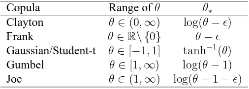
Copula Range ofθ θ∗

Clayton θ_∈(0,_∞) log(θ₋)

Frank θ _∈R_{\ {0} θ−}

Gaussian/Student-t θ ∈[−1,1] tanh−1(θ)

Gumbel θ∈[1,∞) log(θ−1)

[image:7.595.176.429.50.141.2]

Joe θ_∈(1,_∞) log(θ₋1₋)

Table 1: Parameter range of dependence coefficientθfor some classic copula functions and transformations,θ_∗, ofθ

used in optimization. Quantityis set to the machine smallest positive floating-point number multiplied by106

and is used in some cases to ensure that the dependence parameters lie in their respective ranges.

whereψ is the effect of the treatment on the outcome on the scale of the linear predictor, uT_1i = (1, u12i, . . . , u1P1i) is thei

th _{row of U}

1 = (u11, . . . ,u1n)T, the n×P1 model matrix containing

P1 parametric terms (e.g., intercept, dummy and categorical variables), α1 is a coefficient

vec-tor, and the s1k1 are unknown smooth functions of the K1 continuous covariates z1k1i. Varying

coefficient models can be obtained by multiplying one or more smooth terms by some

predic-tor(s) (Hastie & Tibshirani, 1993), and smooth functions of two or more covariates can also be

considered (Wood, 2006). Similarly, uT

2i = (1, u22i, . . . , u2P2i)is thei

th_{row vector of then×P}

2

model matrix U2 = (u21, . . . ,u2n)T, α2 is a parameter vector, and thes2k2 are unknown smooth

terms of the K2 continuous regressors z2k2i. The smooth functions are subject to the centering

(identifiability) constraintPn

i=1svkv(zvkvi) = 0forv = 1,2,kv = 1, . . . , Kv(Wood, 2006).

The smooth functions are represented using the regression spline approach (e.g., Ruppert et al., 2003). Specifically, svkv(zvkvi) is approximated by a linear combination of known spline basis

functions,bvkvj(zvkvi), and regression parameters,βvkvj, i.e.svkv(zvkvi) =

PJ_vkv

j=1 βvkvjbvkvj(zvkvi) =

βT

vkvBvkv(zvkvi), whereJvkv is the number of spline bases used to representsvkv(·), Bvkv(zvkvi)is

theith_{vector of dimensionJ}

vkv containing the basis functions evaluated at the observationzvkvi,

i.e. Bvkv(zvkvi) =

bvkv1(zvkvi), bvkv2(zvkvi), . . . , bvkvJ_vkv(zvkvi)

T

, and βvkv is the

correspond-ing parameter vector. Evaluatcorrespond-ing Bvkv(zvkvi) for eachiyields Jvkv curves with different degrees

of complexity which multiplied by some value of βvkv and then summed will give a (linear or

non-linear) estimate forsvkv(zvkv); see Ruppert et al. (2003) for a detailed overview. Basis

func-tions should be chosen to have convenient mathematical and numerical properties. We employ

low rank thin plate regression splines (Wood, 2003), although many spline definitions (includ-ing B-splines and cubic regression splines) are supported in our implementation. Note that for

one-dimensional smooth functions, the choice of spline definition does not play a crucial role

in determining the shape of ˆsvkv(zvkvi)(Wood, 2006). The cases of smooth terms multiplied by

some covariate(s) and of smooths of more than one variable follow a similar construction; see

Wood (2006, Chapter 4) for full details. Linear predictors (1) and (2) can, therefore, be written as η1i =uT1iα1+BT1iβ1andη2i =ψy1i+uT2iα2+BT2iβ2, where BTvi =

Bv1(zv1i)T, . . . ,BvKv(zvKvi)

T

andβT

v = (βvT1, . . . ,βvKT v). After defining X1i = (u

T

1i,BT1i)Tand X2i = (y1i,uT2i,BT2i)T, we have

η1i =XT1iδ1 andη2i =XT2iδ2 whereδ1T= (αT1,β1T)andδ2T= (ψ,αT2,β2T). Note that the presence

of a binary endogenous variable inη2i does not alter the log-likelihood function presented in the

η2iincludesy1i.

To identify the parameters in η2i, it is typically assumed that an exclusion restriction on the

exogenous variables holds: the regressors in the treatment equation should contain at least one or

more covariates (usually referred to as instruments) not included in the outcome equation.

How-ever, as shown for instance in Han & Vytlacil (2014), Marra & Radice (2011a) and Wilde (2000),

the presence of this restriction may not be necessary.

2.2

Sample average treatment effect

The effect ofy1i on the probability that y2i = 1 is of primary interest. In other words, the aim

is to investigate how the treatment changes the expected outcome. Thus, the treatment effect is

given by the difference between the expected outcome with treatment and the expected outcome

without treatment. Different measures of treatment effect have been proposed in the literature.

Here, we focus on the average treatment effect in the specific sample at hand, rather than that in

the population (SATE; Abadie et al., 2004). In our case, this can be defined as

SATE(δ,X) = 1

n

n

X

i=1

P_{(y2i = 1|y1i = 1)−}P_{(y2i = 1|y1i = 0),}

where

P_{(y2i = 1|y1i = 1) =} C

Φ(η1i),Φ(η2(yi1i=1));θ

Φ(η1i)

,

P_{(y2i = 1|y1i = 0) =} Φ(η

(y1i=0)

2i )− C

Φ(η1i),Φ(η2(yi1i=0));θ

1₋Φ(η1i)

,

the linear predictors are defined in the previous section, η(y1i=r)

2i represents the linear predictor

evaluated at y1i = r for r equal to 1 or 0, δT = (δT1,δ2T, θ), and X = (x1|. . .|xn)T where xi is

defined as(XT_1i,XT_2i)T_{. SATE(δ,X) can be estimated usingSATE( ˆδ,X), whereas a confidence}

interval for it can be obtained employing the delta method. Specifically, the appropriate estimator

of the asymptotic variance ofSATE( ˆδ,X)is

∂SATE(δ,X)

∂δ

T

_δ

=ˆδ

Vδ

∂SATE(δ,X)

∂δ

_δ

=ˆδ

, (3)

where Vδis the covariance matrix ofδ defined in Section 2.4 and

∂SATE(δ,X)

∂δ =

"

∂SATE(δ,X)

∂δ1

T

,∂SATE(δ,X) ∂δ2

T

,∂SATE(δ,X) ∂θ

#T

,

with elements defined in Section S.1 of the online supplementary material. Alternatively, Bayesian

2.3

Parameter estimation

Since the range of θ is bounded in most cases, we use a proper transformation of it, θ∗, and

define δT

∗ = (δT1,δ2T, θ∗), to ensure that in optimization δ∗ ∈ Rp, where p is the total number

of parameters; see Table 1 for ranges ofθ and the transformations employed. Let us denote the

log-likelihood for a given copula function as `(δ∗). Given the flexible linear predictor structure

considered here, unpenalized estimation can result in smooth term estimates that are too rough to

produce practically useful results (e.g., Ruppert et al., 2003). This issue is dealt with by using a

penalty term, such asP2

v=1 PKv

kv=1λvkv

R

s00

vkv(zvkv)

2

dzvkvfor the one-dimensional case, which

measures the second-order roughness of the smooth terms in the model. Theλvkv are smoothing

parameters controlling the trade-off between fit and smoothness and can take values in [0,_∞). Since regression splines are linear in their model parameters, the overall penalty can be written as

βT_S

λβwhereβT = (βT₁,βT₂), Sλ=

P2

v=1 PKv

kv=1λvkvSvkv and the Svkvare positive semi-definite

symmetric known square matrices expanded with zeros everywhere except for the elements which

correspond to the coefficients of thevkth

v smooth term. The expressions for thebvkvj(zvkvi) and

Svkv depend on the type of spline employed and we refer the reader to Ruppert et al. (2003) and

Wood (2003, 2006) for these details. The function to maximize is

`p(δ∗) =`(δ∗)−

1 2β

T_S

λβ, (4)

where the penalty term can be written asδT

∗˜Sλδ∗/2whereS˜λis an overall penalty matrix defined

asdiag(0T_P1, λ1k1S1k1, . . . , λ1K1S1K1,0 T

P2, λ2k2S2k2, . . . , λ2K2S2K2,0)with 0 T

Pv = (0v1, . . . ,0vPv).

2.3.1 Estimatingδ∗ given smoothing parameters

Given λˆT _{= (ˆλ}

1k1, . . . ,λˆ1K1,λˆ2k2, . . . ,ˆλ2K2), we seek to maximize (4). To this end, we use a

trust region approach which is generally more stable and faster than its line-search counterparts,

particularly for functions that are, for example, non-concave and/or exhibit regions that are close

to flat (Nocedal & Wright, 2006, Chapter 4). Leta be an iteration index. Intuitively speaking,

line search methods choose a direction to move frommatoma+1and find the distance along that

direction which gives the best improvement in the objective function. If the function is non-convex or has long plateaus then the optimizer may search far away frommabut still choose anma+1that

is close toma(hence offering a marginal improvement in the objective function). In some cases,

the function will be evaluated so far away frommathat it will not be finite and the algorithm will

fail. Trust region methods choose a maximum distance for the move fromma toma+1 based on

a “trust region” around ma that has a radius of that maximum distance, and then let a candidate

for ma+1 be the minimum of a quadratic approximation of the objective function. Since points

outside of the trust region are not considered, the algorithm never runs too far and/or too fast from

the current iteration. The trust region is shrunken if the proposed point in the region is worse/not

better than the current point; the new problem with smaller region is then solved. If a point which is close to the boundary of the trust region is accepted and it gives a large enough improvement in the

objective function to be undefined or indeterminate, most implementations of line search methods

will fail and user intervention is required. In the trust region approach, the search for ma+1 is

always a solution to the trust region problem; if the function atma+1 is not finite or not better

than the value atma then the proposal is rejected and the trust region shrunken. Finally, a line

search approach requires repeated estimation of the objective function, while trust region methods

evaluate the objective function only after solving the trust region problem. Hence, trust region

methods can be considerably faster when the objective function is expensive to compute. Full

details can be found in (Nocedal & Wright, 2006, Chapter 4).

Let us define the penalized gradient and Hessian at iteration a as g[pa] = g[a] −S˜λˆδ

[a]

∗ and

H[a]

p = H[a]−˜Sλˆ, where g[a] is made up of g

[a]

1 = ∂`(δ∗)/∂δ1|δ₁₌δ[a]

1

, g[₂a] = ∂`(δ∗)/∂δ2|δ₂₌δ[a]

2

and g3[a] = ∂`(δ∗)/∂θ∗|

θ∗=θ [a] ∗

, and the Hessian matrix has a 3× 3 matrix block structure with

(r, h)th_elementH[a]

r,h =∂2`(δ∗)/∂δr∂δhT|δ_r=δ[_ra]_,δ_h=δ[a]

h

,r, h= 1, . . . ,3, whereδ3 =θ∗; details on

the structure of g andH_{can be found in Section S.2 of the online supplementary material. Each}

iteration of the trust region algorithm solves the problem

min

p

˘

`p(δ∗[a])

def

=−

`p(δ[∗a]) +pTg[_pa]+

1 2p

T_H[a]

p p

so that _kp_{k ≤}r[a],

δ[∗a+1]= arg min

p

˘

`p(δ∗[a]) +δ∗[a],

where_{k · k}denotes the Euclidean norm andr[a]_{represents the radius of the trust region. At each}

iteration of the algorithm, `˘p(δ∗[a]) is minimized subject to the constraint that the solution falls

within a trust region with radiusr[a]_{. The proposed solution is then accepted or rejected and the}

trust region expanded or shrunken based on the ratio between the improvement in the objective

function when going from δ∗[a] toδ[∗a+1] and that predicted by the quadratic approximation. The

exact details of the implementation used here can be found in Geyer (2013) who also discusses

numerical stability and termination criteria. Note that, near the solution, the trust region algorithm

typically behaves as a classic unconstrained algorithm.

2.3.2 Estimatingλgivenδ∗

If the model has more than one smooth term per equation, then estimation ofλby direct grid search

optimization of, for instance, a prediction error criterion can be computationally burdensome. It

is therefore pivotal for practical modeling to estimate λ in an automatic way. There are many techniques for automatic multiple smoothing parameter estimation within the penalized likelihood

framework; see Ruppert et al. (2003) and Wood (2006) for detailed overviews. (Note that joint

estimation ofδ∗andλvia maximization of (4) would clearly lead to over-fitting since the highest

value of`p(δ∗)would be obtained whenλˆ =0.)

Let us defineX˜ =X˜1|. . .|X˜n

T

, whereX˜i =diag

XT_1i,XT_2i,1 with X1i and X2i defined in

Section 2.1.1, W[a]as a block diagonal matrix made up of3×3matrices W_i[a]with(r, h)th_element

given by₋∂2_`(δ

∗)i/∂ηri∂ηhi|_η

ri=ηri[a],ηhi=ηhi[a]

withith_{element given by d}[a]

i =

n

∂`(δ∗)_i/∂η_1i|

η1i=η[₁a_i], ∂`(δ∗)i/∂η2i|η2i=η<sub>2</sub>[a<sub>i</sub>], ∂`(δ∗)i/∂η3i|η3i=η[₃a_i]

oT

.

We then have that g[pa] = ˜X

T

d[a]₋S˜λˆδ

[a]

∗ and H[_pa] = −X˜

T

W[a]X˜ ₋˜Sλˆ. Let us use the fact that

close to convergence the trust region algorithm behaves as a classic unconstrained algorithm and

assume thatδ[∗a+1]is a new updated guess. Applying a first order Taylor expansion to g[pa+1]around

δ∗[a], setting the resulting expression to zero, and using the expressions above for gp[a]andH[pa], we

find that

δ∗[a+1]= ( ˜X

T

W[a]X˜ + ˜Sλˆ)

−1_X˜T_W[a]_z[a]_,

wherez[a] ₌

W[a]

−1

d[a]+ ˜Xδ∗[a]. Thusδ∗[a+1]is clearly the solution to the penalized iteratively

re-weighted least squares problem

arg min

δ_∗ k

z+,[a]_−X˜+,[a]_δ∗k2 _+δT_∗˜_Sˆ

λδ∗,

wherez+,[a] ₌√_W[a]z[a]_andX˜+,[a] ₌√_W[a]_{X. In the derivation above, W}˜ [a]_{can also be taken to}

be the expectation of minus the second derivatives of the log-likelihood with respect to the linear

predictors.

From standard likelihood theory,= √WW−1d has mean 0 and covariance (identity) matrix I_{, and} z+ ₌ E₍z+_{) + , where} E₍z+_{) = µz}+ =

√

WX˜δ0

∗, δ∗0 is the true parameter vector

and V₍z+_{) =} V_{() =} I_{. The predicted vector value for z}+ _{is given by µˆ}

z+ = A_λˆz+, where

Aλ =

√

WX˜( ˜XTWX˜ + ˜Sλˆ)

−₁˜

XT√W (known as influence matrix). Following the argumentation

in Wood (2006, Chapter 4),z+ _{will be normally distributed in the large sample limit. Now, the}

smoothing parameters have to be estimated and since the estimated smooth functions should be as close as possible to the respective true functions, it makes sense to estimateλso thatµˆz+ is as

close as possible toµz+. To this end, we employ the expected mean squared error of the model,

which in this case is

E _kµz+ −µˆ_z+k2/nˇ=E kz+−Aλz+−k2

/nˇ

=E _kz+_−Aλz+_k2_/nˇ+E ₋T₋₂T_µ

z+ + 2TAλµz++ 2TAλ

/nˇ

=E _kz+_−Aλz+_k2_{/nˇ−1 + 2tr(Aλ)/n,ˇ}

wherenˇ = 3nand tr(Aλ)represents the effective degrees of freedom (edf) of the penalized model.

The smoothing parameter vector can be estimated by minimizing an estimate of the expectation

above, that is

V(λ) =kz+−_Aλz+k2/nˇ−1 + 2tr(Aλ)/ˇn. (5)

This is equivalent to the expression of the Un-Biased Risk Estimator reported, for instance, in Wood (2006, Chapter 4) as well as to the Akaike information criterion (AIC) after dropping irrelevant constant. The latter equivalence can essentially be seen by noticing that the first term on

In practice, givenδ∗[a+1], we solve the problem

λ[a+1] = arg min

λ V

(λ)def=kz+,[a+1]_−A[_λa+1]z+,[a+1]_k2_{/nˇ−1 + 2tr(A}[_λa+1]_{)/nˇ (6)}

using the automatic approach by Wood (2004), which is based on Newton’s method and can

eval-uate in an efficient and stable way the components in_V(λ)and their first and second derivatives

with respect to log(λ) (since the smoothing parameters can only take positive values). Broadly

speaking, this is achieved using a series of pivoted QR and singular value decompositions which

make the evaluation of the quantities involving A[λa+1], for new trial values ofλ, cheap and

deriva-tive calculations efficient and stable; see Wood (2004) for full details.

2.3.3 Sketch of algorithm

The two steps, detailed in Sections 2.3.1 and 2.3.2, are iterated in a “performance iteration” fashion

(Gu, 2002) until the algorithm satisfies the stopping criterionmax δ∗

[a]

−δ∗[a+1]

< 10

−6_{. The}

steps can be summarized as follows:

step 1 For a given parameter vector valueδ∗[a]and holding the smoothing parameter vector fixed at

λ[a], find an estimate ofδ∗:

δ[∗a+1]= arg min

p

˘

`p(δ[∗a]) +δ

[a]

∗ .

step 2 Construct the working linear model quantities needed in (6) usingδ[∗a+1]and find an estimate

ofλ:

λ[a+1]= arg min

λ V

(λ).

A slight modification of_V(λ)is worth mentioning. If the estimated smoothing parameters yield

curve estimates that are deemed to be too rough and smoother functions are desired then the trace

of the influence matrix can be increased by a factor> 1. Kim & Gu (2004) found, in a different

context, that using as inflation factor of1.4corrects the tendency to over-fitting of prediction error

criteria.

The asymptotic behavior of the proposed estimator and the ensuing formula to calculate the

treatment effect is detailed in Section S.3 of the online supplementary material.

2.4

Confidence intervals and variable selection

At convergence, the covariance matrix ofδˆ∗can be written as Vδˆ_∗ =−H

−₁

p HH

−₁

p . However, the

alternative Bayesian result Vδ_∗ =−H −₁

p can be employed as well. For smooth functions, at finite

sample sizes Vδ_∗ can produce intervals with close to nominal ‘across-the-function’ frequentist

coverage probabilities (Marra & Wood, 2012). This is because the Bayesian covariance matrix

in (3) Vδ rather than Vδ_∗ is needed. This can be easily obtained by using θ in place ofθ∗ when

constructing the covariance matrix.

Point-wise confidence intervals forˆsvkv(zvkvi)can be obtained using

N(svkv(zvkvi),Bvkv(zvkvi)TVδ∗vkvBvkv(zvkvi)), where Vδ∗vkv is the sub-matrix of Vδ∗ that

corre-sponds to the regression spline parameters associated with sˆvkv(zvkvi). Intervals for non-linear

functions of the model coefficients (e.g.,θ,γ and SATE) can be conveniently obtained by

simula-tion from the posterior distribusimula-tion ofδ∗as follows:

step 1 Drawnsim random vectors fromN( ˆδ∗,Vˆδ_∗).

step 2 Calculatensimsimulated realizations of the function of interest. For instance, for a Gaussian

copulaθ = tanh(θ∗), henceθsim = (θ₁sim, θsim₂ , . . . , θ_nsim

sim)where θ

sim

i = tanh(θ∗sim,i ),i =

1, . . . , nsim.

step 3 Usingθsimcalculate the lower, (ς/2), and upper,1₋ς/2, quantiles.

Small values fornsimare typically tolerable. Parameterς is usually set to0.05.

Strictly speaking, point-wise confidence intervals for smooth components are not adequate

for variable selection purposes, although they are often used in practice (e.g., Ruppert et al.,

2003). To test smooth components for equality to zero we use the results by Wood (2013). Let

us define ˆsvkv = Bvkv(zvkv) ˆβvkv, where Bvkv(zvkv) denotes a full column rank matrix, zvkv =

(zvkv1, zvkv2, . . . , zvkvn)

T _{and V}

s_vkv = Bvkv(zvkv)Vδ∗vkvBvkv(zvkv)

T_{. It is then possible to obtain}

approximate p-values for testing smooth components for equality to zero based on

Tr_vkv = ˆsTvkvV

r_vkv−

s_vkv ˆsvkvv˙χ

2

r_vkv,

where Vrvkv−

s_vkv is the rankrvkv Moore-Penrose pseudo-inverse of Vsvkv, which is employed to deal

with possible rank deficiencies. Parameter rvkv is selected using the notion of edf used in (6).

Becauseedf is not an integer, it can be rounded as follows (Wood, 2013)

rvkv =

(

floor(edfvkv) if edfvkv <floor(edfvkv) + 0.05

floor(edfvkv) + 1 otherwise

,

which proved effective in semiparametric bivariate probit models (Marra, 2013). Alternatively,

variable selection can be achieved by adopting a single penalty shrinkage approach as described

in Marra & Radice (2011a) and Marra & Wood (2011).

3

Analysis of health care utilization data

The analysis presented in this section was performed in theRenvironment (R Development Core Team,

2015) using the packageSemiParBIVProbit(Marra & Radice, 2015) which implements the

Variable Definition

Outcome

visits.hosp =1 at least one visit to hospital outpatient departments

Treatment

private =1 private health insurance

Demographic-socioeconomic

age age in years

gender =1 male

race =1 white, =2 black, =3 native American, =4 others

education years of education

income income (000’s)

region =1 northeast, =2 mid-west, =3 south, =4 west

Health-related

health =1 excellent, =2 very good, =3 good, =4 fair,=5 poor

bmi body mass index

diabetes =1 diabetic

hypertension =1 hypertensive on

hyperlipidemia =1 hyperlipidemic

[image:14.595.114.495.56.318.2]

limitation =1 health limits physical activity

Table 2: Description of the outcome and treatment variables, and observed confounders.

3.1

Data

We used a data-set from the 2012 MEPS (http://www.meps.ahrq.gov/) which includes

information on demographics, individual health status, health care utilization and private health

insurance coverage. We excluded individuals younger than 18 years old given their different

overall health profiles and expected usage patterns as compared to those of older individuals.

Individuals who were older than 64 years old were also excluded since the availability of Medicare

obviates the primary insurance decision for almost all US citizens. Individuals that did not have a

complete set of socioeconomic and demographic control variables were excluded from the sample (e.g., missing values for education or income). After exclusions, the final data-set contains 10950

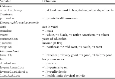
observations. Table 2 summarizes the variables used in the analysis. The choice of these variables

was motivated largely by the findings reported in previous related studies (e.g., Shane & Trivedi,

2012, and references therein).

3.2

Models

Following previous work on the subject (e.g., Holly et al., 1998; Shane & Trivedi, 2012), the equa-tions for private health insurance and health care utilization were specified, inRnotation, as

treat.eq <- private ~ as.factor(health) + as.factor(race) +

as.factor(region) + limitation + gender + diabetes +

hypertension + hyperlipidemia + s(bmi) + s(income) +

s(age) + s(education)

as.factor(region) + limitation + gender + diabetes +

hypertension + hyperlipidemia + s(bmi) + s(income) +

s(age) + s(education)

whereas.factorcoerces its argument to a factor and thes()symbols refer to the unknown

smooth functions described in Section 2.1.1. The smooth components were represented using pe-nalized thin plate regression splines with basis dimensions equal to 20 and penalties based on

second order derivatives (Wood, 2006). In cross-sectional studies, 20 bases typically suffice to

represent well smooth functions, although sensitivity analysis using more spline bases is

advis-able when the effective degrees of freedom of the smooth components are close to the number

of bases used. We also used two alternative spline definitions (i.e., B-splines with second order

difference penalties and cubic regression splines with second order penalties); the resulting

esti-mated curves did not change significantly as compared to those obtained using thin plate splines.

The non-linear specification forbmi, income, age andeducation arises from the fact that

these covariate embody productivity and life-cycle effects that are likely to affect the treatment and outcome non-linearly. In fact, in related studies, Holly et al. (1998) considered a model for health

care utilization that contains linear and quadratic terms inbmi,income,ageandeducation

whereas Marra & Radice (2011b) specified a model containing smooth functions of them.

Consid-ering all copulas discussed in Section 2.1, and including the case in which the outcome equation

is estimated alone (this will be referred to as Independent), we fitted 19 copula models. Based

on theAIC and Bayesian information criterion (BIC) reported in Table 3 the preferred models

are the Gaussian, Gumbel0, Clayton180 and Joe0. After applying the Vuong (Vuong, 1989) and

Clarke (Clarke & Windmeijer, 2012) tests to the four models, it emerged that the Vuong test can

not discriminate among the models whereas the Clarke test favors Gumbel0over the others.

3.3

Empirical results

3.3.1 Measure of dependence

We start off by commenting on the results for the dependence measures of all models fitted (see

Table 3). These represent the association between the unobserved confounders after controlling

for observed confounders. Overall, the models without AIC/BIC support, which account for

a negative dependence, indicate absence of association between the two equations with intervals

which either span all plausible (negative) values forγ/τ or collapse to their point estimates. This

behavior is typically observed when the data are inconsistent with the restrictions on the range

of the dependence parameter, case in which model misspecification should be strongly suspected (e.g., Trivedi & Zimmer, 2005). The models withAIC/BIC support, which account for a

posi-tive dependence, do not exhibit such a behavior and suggest a low association. Interestingly, the

small yet significant dependence parameters obtained for Gumbel0indicates that there exists some

positive association between the unstructured terms of the model equations for private health

insur-ance and hospital utilization which is most likely due to the presence of unobserved confounders.

use health care services as compared to those without coverage.

3.3.2 SATE of private health insurance

The estimated SATE (in%) and confidence interval (CI) for all fitted copula models are reported in Table 3. The Table also reports the estimated SATE for the case in which the unobserved

confounding issue is not taken into account (Independent). Several points are worth noting.

• The chosen models (Gaussian, Gumbel0, Clayton180 and Joe0, which account for a positive

dependence) show similar point estimates with overlapping CIs. The models that account

for a negative dependence (which have no AIC/BIC support) exhibit estimates that are

systematically smaller than those produced by the preferred models (and that produced by

the Independent model). As pointed out in the previous section, the negative dependence

models have estimated dependence parameters that are on the boundary of their parameter spaces, hence suggesting that these models are not supported by the data.

• If the presence of unobserved confounders is not accounted for then the estimated SATE is smaller (4.11%) than that obtained using the chosen models which can control for this issue

(around4.56%). Based on these estimates the direction of the bias appears to be downward.

This result seems counter-intuitive in the sense that if we assume that possible confounders

are allergy and risk aversiveness, then an upward bias should be expected (individuals with

a greater demand for medical care are expected to have a greater demand for insurance).

The explanation behind this apparent contradiction is that employer-provided insurance is

generally limited to full-time workers and is positively related to the worker’s income. The empirical evidence indicates that workers who are in poorer health are less likely to obtain

employer-sponsored coverage (e.g., Buchmueller et al., 2005).

• Using the Gaussian copula the estimated SATE is4.61%, which does not really differ from those obtained using the other supported copula models. This is most likely due to the low

association observed. When γ/τ → 0the copula models converge to the normal product

distribution, case in which all copulas entail very similar distributions. As shown in

simula-tion (see Secsimula-tion S.4 of the online supplementary material), larger differences are likely to

be observed when the association between the treatment and outcome equations is stronger.

In such a scenario, different copulas would entail different distributions (as shown in Figure

1), hence the use of the appropriate copula model can make a difference.

3.3.3 Parametric components

We report the estimated effects for the Gumbel0 copula model. Similar results where obtained

using the other preferred models (these are available upon request).

Most of these effects have the expected signs. Regardinggender, females are slightly more

likely of being hospitalized than males. This may be explained by a higher demand for medical

services among women during their reproductive years (e.g., Sindelar, 1982). As forrace, there

Copula \SATE (95%CIs) γˆ(95%CIs) τˆ(95%CIs) AIC BIC

Independent 4.11 (0.75,7.48) - - 17628.02 18116.06

Gaussian 4.61 (3.15,6.06) 0.39 (0.03,0.64) 0.13 (0.003,0.25) 17621.97 18070.06 Student-t3 4.81 (3.26,6.36) 0.61 (0.38,0.74) 0.34 (0.22,0.45) 17640.29 18085.16

Student-t6 4.56 (2.95,6.16) 0.48 (0.15,0.71) 0.21 (0.08,0.35) 17628.08 18075.64

Student-t9 4.53 (2.95,6.10) 0.44 (0.12,0.74) 0.18 (0.03,0.30) 17624.51 18071.92

Student-t12 4.53 (2.98,6.08) 0.40 (0.07,0.71) 0.16 (0.04,0.29) 17623.01 18070.49

Frank 4.30 (2.92,5.69) 0.29 (0.00,0.55) 0.13 (0.001,0.25) 17622.32 18070.02 Clayton₀ 3.98 (2.62,5.35) 0.11 (0.01,0.73) 0.03 (0.003,0.27) 17624.37 18075.35 Clayton₉₀ 3.97 (2.44,5.49) 0 (-1,0) 0 (-1,0) 17670.23 18263.54 Clayton₁₈₀ 4.52 (3.08,5.96) 0.17 (0.064,0.45) 0.09 (0.03,0.24) 17622.57 18072.41 Clayton₂₇₀ 3.98 (2.21,5.76) 0 (-1,0) 0 (-1,0) 17624.94 18081.31 Gumbel0 4.62 (3.17,6.08) 0.29 (0.09,0.63) 0.13 (0.05,0.31) 17621.05 18069.71

Gumbel90 3.96 (2.42,5.51) 0 (0,0) 0 (0,0) 17672.95 18261.34

Gumbel180 4.02 (2.64,5.40) 0.10 (0.01,0.64) 0.03 (0.001,0.34) 17624.42 18076.04

Gumbel270 3.96 (2.19,5.74) 0 (0,0) 0 (0,0) 17664.94 18280.32

Joe0 4.50 (3.06,5.95) 0.16 (0.04,0.48) 0.09 (0.03,0.26) 17622.66 18072.62

Joe90 3.96 (2.58,5.34) 0 (-1,0) 0 (-1,0) 17670.94 18287.37

Joe180 3.97 (2.62,5.33) 0.04 (0.00,0.80) 0.01 (0,0.54) 17624.76 18079.31

[image:17.595.87.522.52.332.2]

Joe270 3.96 (2.26,5.67) 0 (-1,0) 0 (-1,0) 17669.94 18291.33

Table 3: Estimated SATE (in%), gamma measureγ, Kendall’sτ,AIC andBIC obtained using different copula models for the 2012 MEPS data. 95% confidence intervals for the SATE have been obtained using the delta method detailed in Section 2.2, and those forγandτusing Bayesian posterior simulation as described in Section 2.4. For the Independent model the information criteria have been calculated assuming that the treatment and outcome equations are not associated.

insurance but there is some difference in terms of being hospitalized; black individuals seem to be

less likely to use health care services as compared to whites. This is consistent with the findings

by Shane & Trivedi (2012). Regarding region, residents of the Midwest are more likely to

have a private insurance and to use health care services as compared to those of the Northeast. Individuals’ evaluation of theirhealthstates is a potential predictor of health care utilization.

Those who are in good health are less likely to access health care services. In the same vein,

those who expect themselves to be in good health have little to gain from insurance while those

who are in poor health are more likely to purchase health insurance. The results for the hospital

utilization equation support this hypothesis indicating that the less healthy individuals are, the

more likely they are to be admitted into hospitals. The positive relationship between self-assessed

health and insurance purchase is counter-intuitive to the hypothesis of moral hazard and adverse

selection. However, such finding is not unusual and has been obtained in several previous studies

(see Srivastava & Zhao, 2008, and references therein). The more objective measures of health

status (i.e., diabetes, hypertension and hyperlipidemia) suggest that medical need

is an important determinant of hospital utilization and insurance purchase.

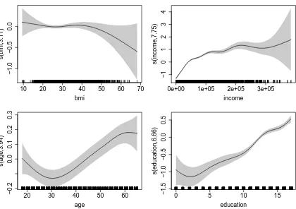
3.3.4 Non-parametric components

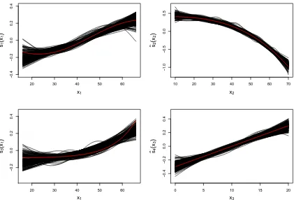
Figures 2 and 3 report the smooth function estimates for the treatment and outcome equations (and

Treatment Eq. Outcome Eq.

Variable Parameter estimate Std. error Parameter estimate Std. error

gender -0.02 0.03 -0.37 0.03

race=2 -0.00 0.04 -0.08 0.04

race=3 0.04 0.15 0.35 0.16

race=4 -0.04 0.05 -0.17 0.07

region=2 0.24 0.05 0.16 0.06

region=3 0.06 0.04 -0.22 0.05

region=4 0.01 0.04 -0.37 0.06

health=2 0.04 0.04 0.10 0.05

health=3 -0.11 0.04 0.33 0.05

health=4 -0.27 0.06 0.48 0.07

health=5 -0.39 0.09 0.67 0.10

diabetes 0.12 0.06 0.06 0.06

hypertension 0.09 0.04 0.09 0.04

hyperlipidemia 0.17 0.04 0.9 0.04

[image:18.595.103.504.69.307.2]

limitation 0.05 0.06 -0.49 0.06

Table 4: Estimated coefficients and standard errors of the parametric components of the Gumbel0model.

10 20 30 40 50 60 70

−1.0

−0.5

0.0

bmi

s(bmi,3.11)

0e+00 1e+05 2e+05 3e+05

−1

0

1

2

3

4

income

s(income

,7.75)

20 30 40 50 60

−0.2

0.0

0.1

0.2

0.3

age

s(age

,3.94)

0 5 10 15

−1.5

−1.0

−0.5

0.0

0.5

education

s(education,6.66)

Figure 2: Smooth function estimates and associated95%point-wise confidence intervals in the treatment equation obtained by applying the Gumbel0regression spline model on the 2012 MEPS data. Results are plotted on the scale

[image:18.595.88.508.394.690.2]

10 20 30 40 50 60 70

−0.2

0.0

0.1

0.2

bmi

s(bmi,1)

0e+00 1e+05 2e+05 3e+05

−0.2

0.0

0.2

0.4

0.6

income

s(income

,1.86)

20 30 40 50 60

−0.3

−0.1

0.1

0.3

age

s(age

,2.13)

0 5 10 15

−0.8

−0.4

0.0

education

s(education,1)

Figure 3: Smooth function estimates and associated 95% point-wise confidence intervals in the outcome equation obtained by applying the Gumbel0regression spline model on the 2012 MEPS data. Results are plotted on the scale

of the linear predictor. P-values for the smooth terms ofbmi,income, ageandeducationare 0.849,0.01,

<0.000and<0.000, respectively.

functions obtained using the other copula models (not reported here but available upon request)

were similar.

The effects ofbmi,income, ageandeducationin the treatment and outcome equations

show different degrees of non-linearity. The point-wise confidence intervals of the smooth

func-tions forbmi in the treatment and outcome equations contain the zero line for the whole range

of the covariate values. The intervals of the smooth forincomein the outcome equation contain the zero line for most of the covariate value range. This suggests thatbmi is a weak predictor of

private health insurance and health care utilization, and thatincomemight not be an important

determinant of hospital utilization. Similar conclusions can be drawn by looking at the p-values

reported in the captions of Figures 2 and 3. As for the remaining variables, the estimated effects

have the expected patterns. For example,ageis a significant determinant in both equations. The

probability of purchasing a private health insurance is found to increase withage. This is

sug-gestive of a higher probability of private health insurance purchase as individuals become older

and less likely to stay healthy (e.g., Hopkins & Kiddi, 1996). The probability of using health care

services also increases withage. Insurance decision as well as health care utilization appear to be highly associated witheducation. Education is likely to increase individuals’ awareness of

health care services and the benefits of purchasing a private health insurance. Higher household

income is associated with an increased probability of purchasing a private health insurance.

equation reported here should be interpreted in a qualitative way only. The actual effects can be

calculated by using simulation or by adapting the formulas of Greene (2012) to the current context.

This would account for the fact that the confounders appearing in the treatment equation have an

indirect effect (through the endogenous variable) on the outcome and a direct effect because they

also appear in the outcome equation.

4

Discussion

We have introduced a framework which can allow researchers to estimate the effect that a binary

treatment has on a binary variable in the presence of unobserved confounding, non-linear covariate

effects and non-Gaussian dependencies between the treatment and outcome equations. We have

provided inferential tools for this framework and presented some argumentation related to the

asymptotic behavior of the proposed penalized maximum likelihood estimator and the ensuing

sample average treatment effect. We have also developed the necessary computational procedures

which are incorporated in theRpackageSemiParBIVProbit(Marra & Radice, 2015).

Using the proposed approach, we have examined the effect of private health insurance on

health care utilization using the 2012 MEPS data-set. There is a generally accepted notion that private health coverage is affected by endogeneity as it is not randomly assigned as in a controlled

trial but rather is the result of individual preferences and health status, such as allergy and risk

aversiveness. Also, the impacts of continuous confounders such as age and education are likely

to be complex since they embody productivity and life-cycle effects that are likely to influence

non-linearly private health insurance and health care utilization. Finally, insurance and health care

utilization may exhibit a non-Gaussian dependence. To our knowledge, no studies have

exam-ined the impact of private health coverage accounting for endogeneity, non-linear contributions of

observed confounders and non-Gaussian dependence between insurance and health care

utiliza-tion, partly due to the lack of appropriate analytical and computational tools. By applying the introduced statistical framework to the 2012 MEPS data we found that not accounting for the

en-dogeneity issue underestimates the effect of private health insurance and that some of the observed

confounder effects are non-linear. We also found that the Gaussian, Gumbel0, Clayton180and Joe0

models were equally supported. This was due to the low yet significant association observed

be-tween the treatment and outcome equations, case in which the copula models entail very similar

distributions. However, as shown in simulation, the use of the appropriate copula model may make

a difference when the association between the two equations is strong.

Since marginal distributions other than Gaussian may be plausible in applications, we explored

the possibility of modeling the margins using skew probit links derived from the standard

skew-normal distribution by Azzalini (1985) as well as the power probit and reciprocal power probit links discussed by Bazan et al. (2010). We opted for these links as they include the probit link

as special case and have desirable mathematical properties. The use of these approaches did not

lead to SATE results different from those reported in Table 3. Moreover, the convergence of the

pointed out by Azzalini & Arellano-Valle (2013), in the simpler context of continuous outcome

variables, having a parameter which regulates the distribution’s skewness enjoys attractive formal

properties from the probability point of view. However, a practical problem in applications is the

possibility that the maximum likelihood estimate of the skewness parameter diverges. That is,

the profile log-likelihood for the skewness coefficient may be flat in a non-negligible portion of

situations. This issue has vanishing probability for increasing sample size, but for finite samples it

occurs with non-negligible probability.

A limitation of the copulas employed in this article is that they are exchangeable (Durante,

2009; Frees & Valdez, 1998; Nelsen, 2007). In the context of our case study, this means that the probability of (not) having private health insurance conditionally to the usage (or not) of health

care services is equal to the probability of using (or not) health care services knowing that a

private health insurance can (not) be used. Following the approach detailed in Frees & Valdez

(1998), we employed the copula_Cκ1,κ2(u, v) =u

1−_κ1

v1−_κ2

C(uκ1_{, v}κ2_{), 0< κ}

1, κ2 <1, which has

the property of including_C as a limiting case. We encountered the same issues mentioned above,

even when using a model with a small number of covariates and without smooth functions.

An interesting avenue for future research includes the use of semi- and non-parametric copula

approaches. These would allow the margins and/or the copula to be estimated non-parametrically

using, for instance, smoothing methods such as kernels, wavelets and orthogonal polynomials. Broadly speaking, if the specification of the model for the margins and copula is correct, then the

parametric approach will outperform semi- and non-parametric methods; however, the reverse will

be true under misspecification. Without any valuable prior information, semi- and non-parametric

techniques should be favored as they will be more flexible in determining the shape of the

under-lying distribution. However, in practice, such techniques are typically limited with regard to the

inclusion of a large set of covariates, may require the imposition of restrictions on the functions

ap-proximating the underlying distribution and may be computationally demanding (e.g., Deheuvels,

1981a,b; Genest et al., 1995; Tutz & Petry, 2013). While a fully parametric copula approach is

less flexible than semi- and non-parametric approaches, it is computationally more feasible and it still allows the user to assess the sensitivity of results to different modeling assumptions.

Another interesting extension would be to consider trivariate system models, controlling for

the endogeneity of the treatment and for non-random sample selection in the outcome (e.g.,

Srivastava & Zhao, 2008). Finally, a future release ofSemiParBIVProbitwill allow the user

to model the copula parameter as a function of a linear predictor to allow for different degrees of

endogeneity across observations; the theoretical and computational framework remains essentially

unchanged.

Acknowledgement

We would like to thank two anonymous reviewers and the Associate Editor for many suggestions

which helped to clarify the contribution of the paper and improved considerably the presentation

References

Abadie, A., Drukker, D., Herr, J. L., & Imbens, G. W. (2004). Implementing matching estimators

for average treatment effects in Stata. Stata Journal, 4, 290–311.

Azzalini, A. (1985). A class of distributions which includes the normal one. Scandinavian Journal of Statistics, 12, 171–178.

Azzalini, A. & Arellano-Valle, R. B. (2013). Maximum penalized likelihood estimation for

skew-normal and skew-t distributions. Journal of Statistical Planning and Inference, 143, 419–433.

Barndorff-Nielsen, O. & Cox, D. (1989). Asymptotic Techniques for Use in Statistics. London:

Chapman and Hall.

Bazan, J. L., H.Bolfarinez, & Branco, M. B. (2010). A framework for skew-probit links in binary

regression. Communications in Statistics: Theory and Methods, 39, 678–697.

Brechmann, E. C. & Schepsmeier, U. (2013). Modeling dependence with c- and d-vine copulas:

The R package CDVine. Journal of Statistical Software, 52(3), 1–27.

Buchmueller, T. C., Grumbach, K., Kronick, R., & Kahn, J. G. (2005). Book review: The effect of

health insurance on medical care utilization and implications for insurance expansion: A review

of the literature. Medical Care Research and Review, 62, 3–30.

Chib, S. & Greenberg, E. (2007). Semiparametric modeling and estimation of instrumental

vari-able models. Journal of Computational and Graphical Statistics, 16, 86–114.

Chib, S. & Hamilton, B. H. (2002). Semiparametric Bayes analysis of longitudinal data treatment models. Journal of Econometrics, 110, 67–89.

Clarke, P. S. & Windmeijer, F. (2012). Instrumental variable estimators for binary outcomes.

Journal of the American Statistical Association, 107, 1638–1652.

Deheuvels, P. (1981a). A kolmogorov-smirnov type test for independence and multivariate

sam-ples. Romanian Journal of Pure and Applied Mathematics, 26, 213–226.

Deheuvels, P. (1981b). A nonparametric test for independence. Pub. Inst. Stat. Univ. Paris, 26,

29–50.

Durante, F. (2009). Construction of non-exchangeable bivariate distribution functions. Statistical

Papers, 50, 383–391.

Frees, E. W. & Valdez, E. A. (1998). Understanding relationships using copulas. North American

Actuarial Journal, 2, 1–25.

Genest, C., Ghoudi, K., & Rivest, L. P. (1995). A semiparametric estimation procedure of

Genest, C., Nikoloulopoulos, A. K., Rivest, L.-P., & Fortin, M. (2013). Predicting dependent

binary outcomes through logistic regressions and meta-elliptical copulas. Brazilian Journal of

Probability and Statistics, 27, 265–284.

Geyer, C. J. (2013). Trust regions.http://cran.r-project.org/web/packages/trust/vignettes/trust.pdf

Gitto, L., Santoro, D., & Sobbrio, G. (2006). Choice of dialysis treatment and type of medical unit

(private vs public), application of a recursive bivariate probit. Health Economics, 15, 1251–

1256.

Goldman, D. P., Bhattacharya, J., McCaffrey, D. F., Duan, N., Leibowitz, A. A., Joyce, G. F., &

Morton, S. C. (2001). Effect of insurance on mortality in an HIV-positive population in care.

Journal of the American Statistical Association, 96, 883–894.

Goodman, L. A. & Kruskal, W. H. (1954). Measures of association for cross classification. Journal

of the American Statistical Association, 49, 732–764.

Greene, W. H. (2012). Econometric Analysis. Prentice Hall, New York.

Gu, C. (2002). Smoothing Spline ANOVA Models. Springer-Verlag, London.

Han, S. & Vytlacil, E. J. (2014). Identification in a generalization of bivariate probit models with

endogenous regressors. Revise and Resubmit, The Journal of Econometrics.

Hastie, T. & Tibshirani, R. (1993). Varying-coefficient models. Journal of the Royal Statistical

Society Series B, 55, 757–796.

Heckman, J. J. (1978). Dummy endogenous variables in a simultaneous equation system.

Econo-metrica, 46, 931–959.

Heckman, J. J., Ichimura, H., & Todd, P. (1997). Matching as an econometric evaluation estimator:

Evidence from evaluating a job training programme. Review of Economic Studies, 64, 605–654.

Holly, A., Gardiol, L., Domenighetti, G., & Brigitte, B. (1998). An econometric model of health

care utilization and health insurance in Switzerland. European Economic Review, 42(3-5), 513–

522.

Hopkins, S. & Kiddi, M. P. (1996). The determinants of the demand for private health insurance

under medicare. Applied Economics, 28, 1623–1632.

Jones, A. M., Koolman, X., & Doorslaer, E. V. (2006). The impact of having supplementary private

health insurance on the uses of specialists. Annales d’Economie et de Statistique, (83/84), 251–

275.

Kauermann, G. (2005). Penalized spline smoothing in multivariable survival models with varying

Kauermann, G., Krivobokova, T., & Fahrmeir, L. (2009). Some asymptotics results on generalized

penalized spline smoothing. Journal of Royal Statistical Society Series B, 71, 487–503.

Kawatkar, A. A. & Nichol, M. B. (2009). Estimation of causal effects of physical activity on

obesity by a recursive bivariate probit model. Value in Health, 12, A131–A132.

Kim, Y. J. & Gu, C. (2004). Smoothing spline gaussian regression: More scalable computation

via efficient approximation. Journal of the Royal Statistical Society Series B, 66, 337–356.

Latif, E. (2009). The impact of diabetes on employment in Canada. Health Economics, 18, 577–

589.

Li, Y. & Jensen, G. A. (2011). The impact of private long-term care insurance on the use of

long-term care. Inquiry, 48(1), 34–50.

Maddala, G. S. (1983). Limited Dependent and Qualitative Variables in Econometrics. Cambridge

University Press, Cambridge.

Marra, G. (2013). On p-values for semiparametric bivariate probit models. Statistical

Methodol-ogy, 10, 23–28.

Marra, G. & Radice, R. (2011a). Estimation of a semiparametric recursive bivariate probit model

in the presence of endogeneity. Canadian Journal of Statistics, 39, 259–279.

Marra, G. & Radice, R. (2011b). A flexible instrumental variable approach. Statistical Modelling,

11, 581–603.

Marra, G. & Radice, R. (2015). SemiParBIVProbit: Semiparametric Bivariate Probit Modelling.

R package version 3.3.

Marra, G. & Wood, S. (2012). Coverage properties of confidence intervals for generalized additive

model components. Scandinavian Journal of Statistics, 39, 53–74.

Marra, G. & Wood, S. N. (2011). Practical variable selection for generalized additive models.

Computational Statistics and Data Analysis, 55, 2372–2387.

McCullagh, P. (1987). Tensor Methods in Statistics. London: Chapman and Hall.

Nelsen, R. (2006). An Introduction to Copulas. New York: Springer.

Nelsen, R. B. (2007). Extremes of nonexchangeability. Statistical Papers, 48, 329–336.

Nocedal, J. & Wright, S. J. (2006). Numerical Optimization. New York: Springer-Verlag.

R Development Core Team (2015). R: A Language and Environment for Statistical Computing. R

Foundation for Statistical Computing, Vienna, Austria. ISBN 3-900051-07-0.

Rosenbaum, P. R. & Rubin, D. B. (1983). The central role of the propensity score in observational