Genetic Algorithms for the Variable Ordering Problem
of Binary Decision Diagrams
Wolfgang Lenders⋆, Christel Baier
Universität Bonn, Institut für Informatik I, Römerstrasse 164, 53117 Bonn, Germany [email protected], [email protected]
Abstract. Ordered binary decision diagrams (BDDs) yield a data structure for switching functions that has been proven to be very useful in many areas of com-puter science. The major problem with BDD-based calculations is the variable ordering problem which addresses the question of finding an ordering of the in-put variables which minimizes the size of the BDD-representation. In this paper, we discuss the use of genetic algorithms to improve the variable ordering of a given BDD. First, we explain the main features of an implementation and report on experimental studies. In this context, we present a new crossover technique that turned out to be very useful in combination with sifting as hybridization technique. Second, we provide a definition of a distance graph which can serve as formal framework for efficient schemes for the fitness evaluation.
1
Introduction
Ordered binary decision diagrams (BDDs for short) are data structures to represent switching functions that rely on a compactification of binary decision trees. More gen-eral, using appropriate binary encodings, BDDs can serve to represent discrete func-tions with a finite domain. They were first introduced by Lee [28] and Akers [1]. In the meantime, various variants of BDDs have been suggested in the literature and applied successfully in many areas of computer science. Most popular are Bryant’s(reduced) ordered binary decisions diagrams [8] that require a fixed variable ordering on any path. They have been proven to be very useful for the verification of reactive systems, often calledsymbolic model checking[32, 10]. Other application areas of BDDs include VLSI design, graph algorithms, complexity theory, matrix-operations, data bases, arti-ficial intelligence, and many more. See e.g. the text books [36, 25, 18, 33, 48].
The crucial point with ordered BDD-based computations is thevariable ordering problem. For a wide range of switching functions, there are polynomial-sized BDDs for “good” variable orderings, while the BDDs under “bad” variable orderings have exponential size. Unfortunately, the problem of finding an optimal variable ordering is NP-complete [45, 6]. However, there are many reordering algorithms that improve the ordering of a given BDD. Most popular are Rudell’s sifting algorithm [41] and the window permutation algorithm [21]. A first attempt to use genetic algorithms for the variable ordering problem for BDDs was presented by Drechsler, Becker and Göckel
⋆The paper is based on material of the diploma thesis by the first author Wolfgang Lenders
[15] where the main genetic operations are partially-mapped crossover and mutation. A related approach using simulated annealing was suggested by Bollig, Löbbing and Wegener [5]. In experimental studies it turned out that these methods yield better re-sults (smaller BDDs) than other dynamic reordering techniques, but they are compa-rably slow, see e.g. [42]. To speed up the computations, several approaches have been suggested, including advanced tricks for the parameter setting and treating sifting as a genetic operation that replaces crossover techniques [16, 46], evolutionary algorithms with learning heuristics [17], the use of computed tables and approximate fitness values [24] or parallel genetic algorithms [12].
The goal of our paper is orthogonal to the above mentioned strategies by present-ing alternative techniques to improve the efficiency and quality of genetic reorderpresent-ing algorithms for BDDs, while still retaining the concept of crossover (in contrast to the approaches of [16, 46]). We concentrate here on the purely genetic part of such reorder-ing algorithms. However, the techniques suggested here can easily be combined with other (non-genetic) methods to increase the efficiency, e.g. by using “ordinary” sifting as in [16, 46].
Unlike [16, 46] which uses inversion as the only genetic recombination technique, we discuss several crossover techniques and present a new one, calledalternating cross-overwhich attempts to maximize the benefits of hybridization, i.e., the combination of a deterministic search algorithm with a genetic algorithm. The idea in the context of BDD minimization relies in generating an interleaving of the parent’s variable order-ings (alternating crossover) and moving the variables with the sifting-technique to the next local optimum after (the hybridization step). Our experimental results show that alternating crossover outperforms other recombination techniques such as order, par-tially matched or cycle crossover and inversion, by means of the BDD-sizes, while no significant differences in the runtime could be observed.
The second contribution is a formal framework to speed up the calculation of the fitness values for the newly generated individuals. In fact, for the variable ordering problem, calculating the BDD-size under a given variable ordering is a time-consuming step. It is typically realized by a sequence of local (level-wise) reorganizations of the BDD, the so calledswap-operator (see e.g. [48]). Even when the final BDD is smaller than the original one, an exponential blow-up for the intermediate BDDs is possible. Thus, strategies that support the fitness calculation of the new population are highly de-sirable. We introduce a formal notion of adistance graph, a weighted graph where the nodes are orderings and the edges are labeled with the minimal number of swaps neces-sary to transform one ordering into another one. Using (variants of) heuristic algorithms for the traveling salesperson problem a “short” tour in the distance graph through the newly generated orderings, for which the fitness values (BDD-sizes in our case) are re-quired, yields an appropriate scheme for the fitness evaluation. The distance graph can also serve as formal framework for other techniques that support the fitness calculation as suggested in [24]. Moreover, the fitness computation via our visiting strategy can easily be modified to weaken the drawback of crossover operations that might lead to unfeasible BDD-sizes, e.g., if they generate individuals that are far from both parents and combine the bad attributes of the parents.
Throughout the paper, we concentrate on the use of our algorithm for the minimiza-tion of ordinary BDDs, but our methods are also applicable to other types of decision diagrams, such as zero suppressed BDDs [36] algebraic decision diagrams, [2, 11] and their normalized version [39], and other DD-variants.
Organization of the paper. The basic concepts of binary decision diagrams and
no-tations used in this paper are summarized in Section 2. Section 3 explains the main concepts of our genetic algorithm and its implementation we used for the experimental studies. Section 4 is concerned with alternating crossover. Our graph-based technique to reduce the runtime for the fitness calculation are described in Section 5. In Section 6, we report on experimental results. Section 7 concludes the paper.
2
Binary decision diagrams
In the remainder of this paper, we fix a finite set
Z
={z1, . . . ,zn}of boolean variables and often refer to the variables by their indices (i.e., we identify indexiwith variable zi). An evaluation forZ
denotes a function that assigns a boolean value (0 or 1) to any variablezi∈Z
. By a switching functionoverZ
, we mean a function f which maps any evaluation forZ
to 0 or 1. Ifz∈Z
then f|z=0and f|z=1denote thecofactorsoff which arise by fixing the assignmentz7→0 andz7→1 respectively. For instance, if f =z1∧(z2∨z3)thenf|z1=0=0 andf|z1=1=z2∨z3.
The fact that there is no data structure for switching functions that is efficient for all switching functions becomes clear from the observation that the number of switching functions over
Z
grows double exponentially in the size ofZ
. Anexplicitrepresentation of switching functions using truth tables seems coherent, but a truth table for a switching function withn variables consists of 2n lines and consequently its space complexity grows exponentially in the number of variables.Implicitdescriptions, like propositional logic formulas and binary decision diagrams can be much more efficient.Binary decision diagrams are a graph based representation of switching functions which rely on the decomposition of switching functions in their cofactors according to theShannon expansion f = (¬z∧f|z=0)∨(z∧f|z=1). Formally, a BDD is an acyclic
rooted directed graph where every inner nodevis labeled with a variable and has two children, called the 0-successor and 1-successor. The terminal nodes are labeled with one of the truth values 0 or 1. In ordered BDDs (OBDD) [8], there is a variable ordering π= (zi
1, . . . ,zin)which is preserved on any path from the root to a terminal node. That
is, ifvis an inner node labeled with variableziℓandwa child ofvwhich is non-terminal and labeled with variablezir thenziℓ appears inπbeforezir, i.e.,iℓ<ir. In the sequel,
we shall use the notationπ-OBDD to denote an OBDD relying on the orderingπand we refer to any inner node labeled with variablezas az-node.
The switching function represented by a terminal node agrees with the correspond-ing constant 0 or 1. The switchcorrespond-ing function of a z-node vwith 0-successor w0 and
1-successorw1is fv= (¬z∧fw0)∨(z∧fw1). The switching function fB represented
by an OBDD
B
agrees with the switching function for its root node. Thus, given an evaluation forZ
, the truth value under fB is obtained by traversingB
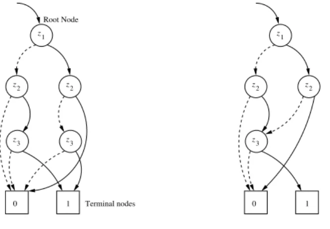
startingin its root and branching in any inner node according to the given evaluation. Fig-ure 1 depicts twoπ-OBDDs with the variable orderingπ= (z1,z2,z3)for the function
1 0 Terminal nodes Root Node 3 z z2 z2 3 z z 1 1 0 3 z z2 z2 z 1
Fig. 1.OBDD and ROBDD
f = (z1∧ ¬z2∧z3)∨(¬z1∧z3∧z2).In the OBDD on the left, bothz3-nodes represent
the same cofactor, namely f|z1=0,z2=1= f|z1=1,z2=0=z3. Thus, a further reduction of
the shown OBDD is possible by identifying the twoz3-nodes which yields thereduced
OBDD(ROBDD) shown on the right. Intuitively, A OBDD is called reduced if it does not contain any redundancies. Formally, an ROBDD
B
denotes an OBDD such that fv6=fwfor all nodesv,winB
withv6=w. Given anπ-OBDD, an equivalentπ-ROBDD is obtained by identifying terminal nodes with the same value, identifyingz-nodes with the same successors and eliminating all inner nodes where the 0- and 1-successor agree. π-ROBDDs yield auniversalrepresentation for switching functions. (This follows from the fact that the above reduction procedure applied to the decision tree for a switch-ing function with orderswitch-ingπyields anπ-ROBDD.) Moreover, the representation byπ -ROBDDs iscanonicalup to isomorphism because the node-set of aπ-ROBDD stands in one-to-one correspondence to the set of cofactors f|zi1=b1,...,zik=bk that can beob-tained from f by assigning values to the “first” variables ofπ.1(Here, the range fork
is 0,1, . . . ,n, andb1, . . . ,bk∈ {0,1}.)
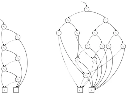
ROBDDs yield a minimized OBDD-representation for a given switching function, provided the variable ordering is viewed to be fixed. However, by varying the ordering πthe size of the BDD can be influenced. Figure 2 illustrates this observation by display-ing two ROBDDs for the same switchdisplay-ing function f = (x1∧x2)∨(y1∧y2)∨(z1∧z2)
using different variable orderings. In the worst case, a ROBDD can have exponential size according to the number of variablesn. There are functions, e.g. the middle bit of multiplication, whose ROBDD representation has exponential size for every variable ordering. Other functions, e.g. the most significant bit of addition, can vary between lin-ear and exponential size depending on the chosen variable ordering while the number of any ROBDD for symmetric functions (e.g.n-ary disjunction or the parity function) is at most quadratic. See [9] and e.g. the text books [33, 48] for a detailed discussion of the complexity of ROBDDs.
2 z y2 x x1 y1 1 z 1 0 2 x 1 y1 1 z 1 z y1 x2 1 z x2 x2 1 z x2 y 2 2 z 1 0 y 2
Fig. 2.Two BDDs for the same switching function using different variable orderings
Shared BDDs. Most BDD-packages follow the approach of [35] who suggested the
si-multaneous representation of several switching functions in one reduced graph (called sharedormulti-rooted BDD) where the ROBDDs of the represented functions are re-alized as subgraphs and share the nodes for common cofactors. With several additional implementation tricks (appropriate hash tables, the ITE-operator to treat all boolean connectives, negated edges, etc.) the manipulation of switching functions and other BDD-based calculations can be realized efficiently, such as checking equivalence of switching functions in constant time or performing boolean combinations in time poly-nomial in the sizes of the ROBDDs for the arguments.
Throughout the paper the term BDD will refer to a shared BDD with negative edges. (This also applies for the number of BDD-nodes in the experimental results.)
The Variable Ordering Problem. For the wide range of functions where the
BDD-sizes range from polynomial to exponential, the variable ordering has an immense im-portance for BDD-applications, not only for reasons of memory requirement but also for the runtime of BDD manipulation operations. Beside some heuristics that compute a variable ordering from a given circuit description there is a wide range ofdynamic reorderingalgorithms that attempt to improve the given variable ordering. The problem of finding an optimal variable ordering for a given BDD is known to be NP-complete [45, 6]. The best known algorithm that determines an optimal variable ordering requires exponential time [20]. However, there are several Greedy-heuristics that might return a suboptimal ordering. All these reordering algorithms are based on sequentially ex-changing pairs of neighboring variables. This basicswapoperation induces only local changes to the involved variables and can be carried out in constant time for each node
that has to be handled. Thus, the running time of the operationswap(z,z′)on the BDD
B
with orderingπ, wherezandz′are adjacent inπ, is linear in the number ofz-nodes and the number of their incoming edges inB
. Using appropriate sequences of swap operations, any variable ordering can be transformed into another one.One of the most commonly used deterministic heuristics for BDD minimization is Rudell’ssiftingalgorithm [41] . The basic idea of sifting is to move each variable suc-cessively through the whole variable ordering and eventually leave it at the position that yields the best BDD size. This procedure can be repeated as long as the variable order-ing changes (iterated siftorder-ing). Several additional heuristics can be used to improve the efficiency of the sifting algorithm. Most popular is the use of amaximum growth factor cwhich stops the movement of a variable in one direction if the BDD-size becomes c-times larger than the original one. In our genetic algorithm, we shall use (non-iterated) sifting as hybridization technique with small maximum growth factorsc. With such a choice forc, the sifting procedure is quite fast and searches the local optimum for any variable in its neighborhood. In fact, we made good experience with alocal searchthat we obtain by choosing max growth factorc=1.
Genetic algorithmsfor the variable ordering problem rely on a representation of the variable orderings in permutation form. The main genetic operations used in the algo-rithm proposed in [15] are (i)partially matched crossover(PMX) [22] which selects a matching section between two cutpoints and uses exchange operations to make one parent’s matching section assimilate the other’s, (ii)mutationwhich exchanges the po-sitions of two variables, and (iii)inversion[26] which selects at random two cutpoints and reverses the ordering in the enclosed segment. To improve the efficiency, [16, 46] suggest to skip crossover techniques and use sifting as a “normal” operation instead,2 while [12] deals with a parallel genetic algorithms with PMX and mutation as main operations. Other additional techniques to achieve a speed-up are proposed in e.g. [24]. Our approach where sifting serves as hybridization technique should be contrasted to the approach of [16, 46] where sifting serves as a “normal” operation which is chosen with a probability of 50% and executed with the maxgrowth factorc=2. In our setting, we deal with a minimized version of sifting that only serves for a local search in the surrounding of an offspring generated by a crossover operation. In fact, by choosing the maxgrowth factorc=1 we only look for the nearest local optimum of any variable which makes the sifting-phase much faster than with higher maxgrowth factors (such asc=2).
3
A genetic algorithm for the variable ordering problem
In this section, we summarize the main features of our implementation of a genetic algorithm for the BDD minimization problem. We realized the standard schema for evolutionary algorithms with hybridization, sketched in Figure 3, using several genetic 2More precisely, the main “proper” genetic operation in [16, 46] is inversion, but they skip the
crossover techniques, and use mutation only if the offspring is equal to the parent element. In [16] some additional problem-specific recombination and mutation operators have been used for incompletely specified boolean functions. As we shrink our attention to completely specified function these techniques are not applicable in our setting.
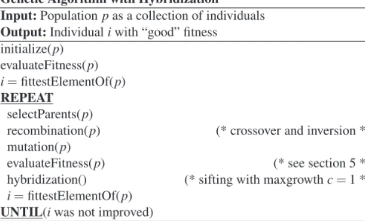
Genetic Algorithm with Hybridization Input:Populationpas a collection of individuals
Output:Individualiwith “good” fitness initialize(p)
evaluateFitness(p) i=fittestElementOf(p)
REPEAT
selectParents(p)
recombination(p) (* crossover and inversion *) mutation(p)
evaluateFitness(p) (* see section 5 *) hybridization() (* sifting with maxgrowthc=1 *) i=fittestElementOf(p)
UNTIL(iwas not improved)
Fig. 3.A hybrid genetic algorithm
operations. We adapted several techniques for evolutionary algorithms suggested some-where else in the literature and developed a new crossover technique (see Section 4) as well as a graph-algorithmic approach for the design of an efficient schema for the fitness computation (see Section 5).
The population size is parametric in our implementation. Even for large circuits, we made good experience with small population sizes, such as 8 individuals per population (see Section 6). The initial population is chosen at random. Techniques that derive a promising ordering from the topology of a circuit description (e.g. the fanin heuristic [30] or weight heuristic [35]) could be used in addition. Also an improvement of the initial population with deterministic reordering algorithms (such as sifting or window permutation) could be integrated, as e.g. in [15].
Recombination. Beside the partially matched crossover (PMX) [22], which is also
used in [15] and [12], we consider three other crossover techniques.Order crossover [13] choosesn/2 pairwise different positions and copies the genes at the selected posi-tions to the offspring, and finally, fills up the gaps using the missing genes in the order they are found in the second parent. In general, the offspring under order crossover assimilates the first parent more than the second. Another version of order crossover in-corporates cutpoints instead of randomly selected positions. Every element between the two cutpoints is copied from the first parent, the elements outside the cutpoints are filled up with the missing elements, preserving the second parents’ order. This variant has the benefit of being less disruptive.Cycle crossover[38] attempts to retain the original posi-tion of genes in their parents. This is achieved by continuous copying of genes from one parent until the end of a cycle is reached, then switching and continuing from the other parent. In rare occasions the offspring can be equal to one of its parents. This case has to be combined with forced mutation to achieve a modification in the next generation. In addition, we implementedalternating crossover, that will be explained in Section 4,
and theinversionoperator [26], which reverses the fragment of a given variable ordering between randomly chosen cutpoints, as an asexual recombination technique.
Mutation. Mutation of a permutation means the exchange of the positions of two
vari-ables by appropriate swap-operations. The approach we have chosen in our implemen-tation first takes a general decision whether a given offspring is to be mutated or not. If so, a level of mutation is chosen and expressed as a number of variable exchanges to be executed. The positions of the variables to be exchanged are picked randomly, also multiple selection of the same variable is possible. This approach is efficient in implementation and execution, and it resembles the original mutation scheme. A forced mutation in case a crossover does not generate (enough) differences between offspring and parents is available. For measuring “differences”, adistanceis defined in Section 5.
Fitness scaling. Choosing the BDD size as a natural measure for the fitness of a
vari-able ordering seems straightforward. Nevertheless the fitness values will be “negated”, conducted by settingfitness(π) =max_bdd_size_found−bdd_size(π), for implemen-tation reasons, which also retains the comfort of speaking of ahigherfitness as a better one, whereas a higher BDD size would imply a worse variable ordering. In Section 5, we will explain our new scheme to minimize the number of swaps necessary for fitness calculation by a distance minimizing strategy.
To handle the problem of premature convergence3or the problem of fitness values that are too close to each other (which can happen in “late” populations, also in the non-premature case, in particular for small population sizes), we adapt the approach of Goldberg [23] and use alinear scaling mechanism. That is, we replace the original fitness function f by the scaling functionf′=a f+bby first fixingf′(avg)tof(avg), which ensures that each not less than average individual obtains a scaled value≥1 and is therefore guaranteed a mating opportunity in a subsequent remainder selection scheme. Toward the end of a GA’s run, the population has largely converged. In this environment, the maximum fitness is generally close to the average fitness, whereas recombination may generate lethals, i.e. individuals with a far below average fitness. These individuals are likely to be scaled to negative fitness values. These exceptions are caught and the affected individuals set to zero fitness. The resulting fitness values are sampled usingstochastic universal sampling[3, 4] by default, while other sampling methods, such as roulette wheel selection or remainder sampling with or without re-placement, are available upon selection.
A variant with the full sifting procedure. As pointed out in [16, 46], the efficiency
of evolutionary reordering algorithms as in Fig. 3 can be increased by using “ordinary” sifting (with large maxgrowth factor, sayc=2) as an alternative in the recombination phase. As mentioned before, the aim of our paper is to study the gain of the proper genetic operators, and therefore, we do not consider this option here.
3Premature convergence e.g. occurs if in the initial population one of the randomly selected
individuals represents a fairly good solution already which is far away from the other individ-uals and if this “superhero” is chosen multiple times for mating and is going to spread its genes throughout the population instantly.
Alternating Crossover
Input:Parentsp1andp2of lengthn Output:Offspringπ done={ } candidate=p1.atPosition(0) position_p1=0 position_p2=0 FOR(i=0)TO(i=n−1)DO WHILE(candidate∈done)DO
IF(i mod 2=0)THEN
candidate=p1.atPosition(position_p1) position_p1=position_p1+1
ELSE
candidate=p2.atPosition(position_p2) position_p2=position_p2+1 FI OD done∪ {candidate} π.atPosition(i)=candidate OD returnπ
Fig. 4.Alternating Crossover
4
Alternating crossover
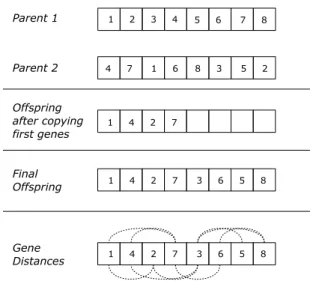
We suggest a new crossover technique, called alternating crossover, which in combina-tion with sifting as hybridizacombina-tion technique turned out to be very successful. Alternating crossover generates offspring by copying genes alternately from the parents and inter-leaves them this way. See Figure 4. This creates offspring in which genes that were ad-jacent in one parent are generally separated by one or more genes from the other parent. Under normal circumstances this disruption of schemata would be considered harmful, but in conjunction withsiftingwith maxgrowth factorc=1 as hybridization algorithm it bears good results. Sifting performs swaps of neighboring variables and retains the exchange if it was beneficial. This way, every separation of genes introduced during the application of alternate crossover can be revoked if necessary, while on the other hand many genes are tested in the surroundings of their current position. Therefore, alter-nating crossover in conjunction with sifting exploits the offspring’s local neighborhood thoroughly.
Figure 5 depicts an example of an alternating crossover application and highlights the genes in the offspring that were adjacent in a parent and are now insifting distance, i.e. their distance is less than 2. Thus even our minimized sifting procedure is able to restore the original ordering if necessary. (Here, we identify variablezi with its index i.) We call two genesaandbin sifting distance, when they can be made adjacent by no more than two exchanges of neighboring genes, i.e. when there are at most two genes
Fig. 5.Example for the operation ofAlternating Crossover
betweenaandb. Our minimized sifting procedure moves each gene at least one step in each direction and is therefore able to recover the original ordering should it have been the most beneficial one. In the following example, let the original ordering with adjacent genesaandbbe better than the newly generated one:
original ordering: x a b y newly generated by alternating crossover: a x y b exchange neighboring variablesaandx: x a y b exchange neighboring variablesbandy: x a b y
Since we said the original ordering to be the most beneficial one, sifting would have executed exactly these two variable exchanges.
5
Fitness calculation via an optimized visiting order
Obtaining the actual fitness value for a variable ordering involves generating the cor-responding binary decision diagram via an appropriate sequence of swap-operations. This can be a costly procedure if the ordering differs clearly from the current order. To minimize the number of swaps necessary for fitness calculation we suggest a strategy that attempts to find an efficient visiting order of the individuals of the new population (variable orderings) for which the fitness values (BDD-sizes) are still unknown.
In principle, fitness can be calculated at different times during the run of a genetic algorithm. Calculating fitness for each individual directly after it has been generated has
the benefit of being able to decide about the individual’s fate at once. If, for example, the offspring generated by a crossover is way worse than its parents it can be discarded in favor of the better parent. On the other hand, this approach does not allow alterations in the order the offspring is tested, which otherwise can be optimized. In the sequel, we explain a strategy to optimize the visiting order of the individuals by providing a formal definition for the distance between variable orderings.
A distance function for variable orderings. In the sequel, we identify any
swap-operation with the index of the variable to be swapped with its right neighbor. Thus, for a variable set
Z
={z1, . . . ,zn}of cardinalityn, we denote any swap-operation by an integers∈ {1, . . . ,n−1}. We writeπ⊲sπ′to denote that swap-operationstransforms the variable orderingπinto the variable orderingπ′. By aswap sequence, we mean any finite sequenceσ= (s1,s2, . . . ,sl)of swap-operations. We refer to|σ|=las the length ofσ.σis said to transformπintoπ′, denotedπ⊲σπ′, if the sequential composition ofthe swapssitransformsπtoπ′, i.e.,
π⊲σπ′ if π⊲s1π1⊲s2π2. . .⊲s lπl=π
′.
σis called aminimum swap sequencefor(π,π′)ifσtransformsπtoπ′ and if there
is no shorter swap sequence thanσthat also transformsπtoπ′. The distanceδ(π,π′)
between two variable orderingsπandπ′is defined as the length of a minimum swap
sequence for(π,π′). That is,δ(π,π′) =min
|σ|:π⊲σπ′ .
Proposition 1. δis a metric on the the set of variable orderings. That is,
1. δ(π,π′) =0ifπ=π′
2. δ(π,π′) =δ(π′,π)
3. δ(π,π′)≤δ(π,πˆ) +δ(πˆ,π′)
The proof of Proposition 1 is straightforward and omitted here. The orderings with maximum distance between each other are the pairs π,π−1
, wereπ−1is the inverse ordering ofπ.
Proposition 2. If πandπ′ are variable orderings for a variable set of cardinality n
then
δ(π,π′) ≤ δ(π,π−1) =n(n−1) 2
Proof. The fact thatδ(π,π′) ≤ (n−1) + (n−2) +. . .+1=n(n−1)
2 is clear as we may
consider the swap sequence which first moves the last variable ofπ′with at most(n−1)
swaps at positionn, then moves the variable at positionn−1 inπ′with at mostn−2
swaps at its final positionn−1, and so on.
It remains to provide the argument why no swap sequence shorter thann(n2−1) trans-formsπintoπ−1. Letπandπ′be arbitrary orderings for variablesz
1, . . . ,znandkithe number of variableszjsuch thati6=jand (i)zioccurs inπbeforezjand (ii)zjoccurs inπ′ beforezi. That is,π= (. . . ,zi, . . . ,zj, . . .)andπ′= (. . . ,zj, . . . ,zi, . . .). Then, any swap sequence that transformsπintoπ′has to perform at leastkiswaps that exchange ziwith its right neighbor. Thus,δ(π,π′)≥k1+. . .+kn. In the case,π′=π−1, we have ki=n−i, Thus,δ(π,π−1)≥(n−1) + (n−2) +. . .+1=n(n−1)/2.
1 2 1 3 1 2 3 2 2 1 2 2 1 3 1 321 123 312 231 213 132
Fig. 6.A distance graph for orderings with three variables
Deriving an efficient fitness calculation scheme from the distance graph. The above
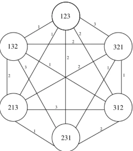
proposition shows that inversion, a powerful genetic operation, requires a number of swaps quadratic to the length of the inverted segment. This makes an immediate fitness rating of the offspring less desirable in comparison to the opportunity to optimize the order of visiting the individuals. Our strategy for reducing the number of variable swaps, that have to be carried out for computing all fitness values by finding an advantageous visiting order for the individuals, is based on adistance graph, a complete graph where the individuals for which the fitness still has to be computed form the vertices, while the edge between two verticesπ1andπ2is marked with their distanceδ(π1,π2). (Because of the symmetry ofδ the distance graph can be viewed as an undirected graph.) An example for a distance graph for three variables4is provided in Figure 6. Usually, the distance graph will not contain allpossible vertices as suggested by the figure, but only those vertices coding for members of the group of offspring whose fitness is still unknown.
Now we could ask for anoptimal visiting strategyfor the individuals, i.e. a visiting order that visits all nodes of the distance graph and which minimizes the sum of all covered distances (the total number of swap operations which have to be carried out). Since we are looking at an instance of the traveling salesperson problem, the question for an optimal visiting order is computationally hard (NP-complete). Instead, we may adapt any heuristic algorithms for the TSP to obtain an efficient, possibly sub-optimal visiting order of the vertices in the distance graph. In our implementation, we employed thenearest neighbor heuristic[34] to decide which individual is to be considered next until all fitness values are computed. Our experiments showed that this procedure means a major speed-up towards the regular visiting order, because the calculation of fitness 4Again, we identify any variable with its index. E.g., node 123 stands for the orderingπ=
values is one of the most time-consuming but basic and irreplaceable parts of the mini-mization algorithm.
A variant of the graph-based visiting schema. [16, 46] observed the problem that
variable orderings generated by the standard crossover techniques (PMX, OX or CX) might lead to BDDs of unfeasible size. To avoid this problem, we suggest the following variant of our visiting algorithm. If during the execution of a minimum swap sequence from one vertexπto another vertexπ′of the distance graph the BDD-size is larger than a certainthresholdthen we may discardπ′and, if necessary, generate a new variable or-deringπ′′via genetic operations (recombination, mutation and sifting as hybridization technique). In this case, of course, the visiting strategy has to be revised dynamically. The threshold can either be a fixed upper bound for the BDD-size or can be determined by a function depending on the fitness values that are already known. Another alterna-tive for the threshold is to use a maxgrowth factor (as it is standard for sifting) for the swap sequences that are executed in the visiting strategy.
In addition, the best intermediate ordering ˆπ, obtained by executing the minimum swap sequence from nodeπto nodeπ′in the distance graph, can be used as an additional
candidate for the next generation, provided it is better thanπandπ′.
Integration of other advanced techniques. Our graph-algorithmic approach for the
fitness computation can easily be modified to integrate the three methods suggested by Günther and Drechsler [24] to accelerate evolutionary algorithms for sequencing problems.
(1) For an approach where the BDDs forseveral variable orderingsare stored to speed up the fitness calculations (as proposed by [24]) we may also deal with a distance graph, but now equipped with another weight function for the edges. Letπ1, . . . ,πm be the variable orderings for which corresponding BDDs are stored. Then, we may use the weight function ˆδ(π,π′) = minδ
(π,π′), δ(πi,π′):i=1, . . . ,m which captures the possibility to start the computation of the π′-BDD with one of the stored BDDs rather than theπ-BDD.
(2) Following [24], we may also use computed-tablesthat store the BDD-sizes for already considered variable orderings. In our setting, this means a simplification of the distance graph which only contains the orderings not considered so far. (3) The third method suggested in [24] relies on the use of upper and lower bounds
for the BDD-sizes that will be obtained through local modifications of the ordering [7]. As shown in [24], this technique in combination with multiple representation as in (1) and computed-tables as in (2) can lead to a speed-up around 80%. This idea can be integrated in our graph-based approach by choosing a constantdand modifying the visiting strategy as follows: If the current node isπthen we use such approximate fitness valuesrather than the precise BDD-sizes for all (possibly, but one) orderingsπ′withδ(π,π′)≤d.
6
Experimental results
To evaluate the performance of the several recombination techniques (crossover, inver-sion) and the influence of the parameter setting, we implemented the schema sketched
benchmark original inputs outputs BDD size apex1 6785 45 45 apex2 13418 38 3 apex3 53365 54 50 apex4 1040 9 19 apex5 3944 114 88 apex6 1993 135 99 apex7 1775 49 37 comp 203198 32 3 cps 1869 24 109 dalu 11178 75 16
benchmark original inputs outputs BDD size des 10771 256 245 duke2 596 22 29 e64 1500 65 65 ex4p 994 84 28 i5 1032 133 66 i6 388 138 67 i7 559 199 67 i8 10366 133 81 vg2 735 25 8 Fig. 7.Benchmarks
in Fig. 3. For all tests we used excerpts of the LGSynth93 benchmark suite (see Fig. 7), obtainable from [31]. We carried out ten runs of our genetic algorithm and present the average BDD size as well as the best result we obtained, in order to visualize the vari-ation in the results. The indicated time shows CPU seconds on a Pentium IV 2.4 GHz PC with 512 MB of RAM running the JJS-BDD package [27] on Linux.
Unless stated otherwise, in all tests the parameters of our genetic algorithm were chosen as follows. The population size is 8, the maxgrowth factor for hybrid sifting isc=1. We carried out experiments with growth factors of 1.1 and 1.2 (not shown here), which resulted in almost identical5results, but bearing a longer runtime. For the
selection method, we used stochastic universal sampling and realized the concept of elitarism for one individual.
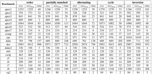
Comparison of the crossover operators. To compare the types of crossover (OX,
PMX, CX and AX) and inversion, we restricted our algorithm to the use of a single operator. An inspection of the results for the five operators in Fig. 8 yields that the runtimes all assimilate each other. To compare the quality of the results we take only the best BDD size achieved during the ten runs into account.
order partially matched alternating cycle inversion
11 14 17 7 7
The above table illustrates for how many benchmark circuits each crossover yielded a best result. (If more than one crossover achieved the best result we awarded a point to each of them.) Thus, alternating crossover bears the best results, followed by partially matched crossover. The combination of different crossover operators is, however, the most promising approach, since the sequential application of different crossovers on the same individual allows more possible outcomes than repetitive application of the same operator. This can also be seen from the results shown in the left column of Fig. 10.
5One benchmark resulted in a BDD two nodes smaller.size
avg results were slightly better in
order partially matched alternating cycle inversion Benchmark
size sizeavg time size sizeavg time size sizeavg time size sizeavg time size sizeavg time
apex1 1253 1255 40 1246 1258 52 1250 1253 39 1270 1270 33 1246 1253 101 apex2 354 372 32 318 327 54 328 338 22 321 345 23 392 395 22 apex3 841 841 20 839 841 28 839 841 23 841 841 20 840 841 30 apex4 889 889 2 889 889 2 889 889 2 889 889 2 889 889 2 apex5 1044 1044 85 1044 1050 113 1044 1044 72 1073 1082 50 1086 1092 68 apex6 523 532 58 513 527 89 510 531 55 524 531 78 575 587 81 apex7 214 214 6 214 214 6 214 214 6 216 217 5 214 214 6 comp 101 107 33 110 125 28 101 110 36 122 144 37 143 143 20 cps 971 971 18 971 972 12 971 974 13 977 976 10 1010 1010 14 dalu 785 798 157 689 689 248 689 701 138 689 689 205 699 711 192 des 2983 3012 988 2971 2977 723 2958 2974 756 2992 3015 601 2987 2992 953 duke2 336 336 3 336 336 4 336 336 4 336 352 3 336 336 4 e64 129 129 12 129 129 12 129 129 12 129 129 11 129 129 16 ex4p 463 468 16 466 471 26 459 470 16 460 481 17 465 468 21 i5 134 134 17 134 134 16 134 134 18 134 134 18 134 134 35 i6 209 209 14 209 209 15 209 209 15 209 209 14 209 209 14 i7 334 334 39 333 333 59 333 335 50 334 335 52 335 335 38 i8 1277 1280 163 1280 1281 196 1277 1281 149 1285 1344 150 1280 1281 206 vg2 80 80 2 80 80 2 80 80 2 84 84 2 84 84 3
Fig. 8.Comparison between five recombination operators
For several benchmarks the best result is obtained using a combination of crossovers, inex4pfor example, the combination reaches a BDD size of 242 BDD nodes, while the best result of a single operator, in this case alternating crossover, is 459 BDD nodes. Other examples for the superiority of a combination of crossovers to the use of a single operator areapex1,apex3,companddes.
Given our results on the comparison of the recombination techniques (Fig. 8), we argue that the restriction to inversion as the only proper genetic operation in the re-combination phase as suggested in [16, 46] shrinks the gain of evolutionary reorder-ing techniques. The motivation given in [16, 46] for omittreorder-ing crossover techniques was their excessive runtime requirements. However, a comparison of the the time-columns in Fig. 8 shows that – in combination with our graph-based fitness evaluation technique – the crossover techniques are in average no worse than inversion. (Additionally, the generation of too large BDDs can be prevented as described in Section 5.)
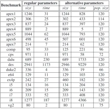
Parameter setting. To illustrate the benefits of our parameter setting and graph-based
fitness evaluation technique, we performed tests where we used the parameter setting used in [15]. Here, the population size is set to min{120,3·population size}. The max-imum growth factor for hybrid sifting is set toc=2. Elitarism is applied to the better half of the population. The results in Figure 9 demonstrate that the alternative choice of parameters rarely achieves a better result than our choice. The best result, obtained for benchmarkapex2, is only four nodes smaller than our result. On the other hand, the alternative parameters results in a runtime which exceeds ours generally by factor 10 to 20. In summary, as Figure 9 shows, our genetic algorithm with crossover and the graph-based visiting strategy performs very well, already with a small population size.
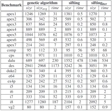
Comparison of our genetic algorithm with “pure sifting”. For a comparison of the
schema in Fig. 3 which only uses crossover (but no inversion) against deterministic re-ordering heuristics, we assigned probability 0.6 to alternating crossover, and 0.2 to both
regular parameters alternative parameters Benchmark
size time size time pop.size
apex1 1246 31 1244 828 120 apex2 306 25 302 433 114 apex3 837 24 837 397 120 apex4 889 2 889 5 27 apex5 1044 62 1044 793 120 apex6 498 45 507 601 120 apex7 214 7 214 62 120 comp 95 33 125 221 96 cps 971 11 971 58 72 dalu 689 230 689 1733 120 des 2941 1173 2946 9229 120 duke2 336 4 336 19 66 e64 129 11 129 103 120 ex4p 242 27 460 182 120 i5 134 16 134 204 120 i6 209 15 209 143 120 i7 333 52 333 408 120 i8 1277 187 1277 4366 120 vg2 80 2 80 11 75
Fig. 9.Regular versus alternative parameters
partially matched and cycle crossover. We obtained similar results when cycle crossover is replaced with order crossover or when assigning the same weight to them. As before, the maxgrowth factor for hybrid sifting is 1. On the other hand, we considered sifting and iterated sifting with maxgrowth factor 1.3. Using our genetic algorithm, the result-ing BDD in general is considerably smaller than it is after application of siftresult-ing. In some examples likeapex2anddaluwe even achieve a bisection of the BDD’s size. In no case is the best result of ten GA runs worse then the result achieved by sifting. This positive result is obtained at the expense of runtime, which in average is an order of magnitude higher than it is for sifting, on the other hand for benchmarkscompanddalu the runtimes for sifting even exceed those of our GA. In average, however, runtime for our GA is longer, though it generates a substantially smaller BDD.
In his diploma thesis [29], the first author also reports about experiments with the window permutation algorithm [21]. The obtained results agree with the common obser-vation that window permutation is fast but a rather weak minimization heuristic. Thus, our genetic algorithm yields much better results in terms of quality, in some cases, like comp,desanddalufor instance, the BDD-sizes were even only a fraction (<1%) of those returned by window permutation, on the price of a longer computation time.
genetic algorithm sifting siftingiter
Benchmark
size sizeavg time size time size time
apex1 1246 1269 31 1381 0.5 1270 3 apex2 306 342 25 589 0.5 502 2 apex3 837 864 24 851 0.2 850 0.8 apex4 889 889 2 889 0.1 889 0.1 apex5 1044 1076 62 1076 0.7 1073 2 apex6 498 569 45 532 0.6 520 3 apex7 214 241 7 297 0.1 248 0.2 comp 95 112 33 95 56 95 68 cps 971 971 11 1010 0.2 1010 0.3 dalu 689 697 230 1552 478 1346 534 des 2941 2968 1173 3242 36 3051 39 duke2 336 340 4 395 0.1 360 0.3 e64 129 129 11 155 0.2 129 0.4 ex4p 242 242 27 512 0.2 507 0.6 i5 134 134 16 134 0.3 134 0.6 i6 209 209 15 215 0.3 209 2 i7 333 334 52 335 0.9 335 2 i8 1277 1280 187 2104 2 2092 5 vg2 80 80 2 157 0.1 152 0.9
Fig. 10.Comparison between our genetic algorithm and sifting
7
Conclusion
The goal of the paper was to study in detail the gain of genetic operations in the context of dynamic reordering algorithms for BDDs. We discussed several crossover variants and suggested a new one, called alternating crossover, which turned out to be very useful in combination with a “minimized version” of sifting as hybridization technique. In addition, we proposed a graph-algorithmic approach to speed up the fitness evaluation which, in case of the variable ordering problem for BDD, is a time-consuming step. In contrast to the observations made by [16, 46] our experiments (see Section 6) show that a random selection between crossover techniques and inversion yields better results than the sparse use of “proper” genetic operations as in [16, 46].
Using the proposed techniques, runtime requirements for genetic reordering algo-rithms were brought down to a reasonable level, although, concerning the computation time, our techniques are still not competitive to deterministic reordering heuristics such as sifting or window permutation. However, our approach nicely fits in the framework of Drechsler et al. [16, 46] who pointed out that the mixture of genetic techniques with ordinary sifting yields a good balance between speed and quality, as it captures the advantages of both genetic algorithms and comparably fast deterministic reordering algorithms. In addition, we explained that other methods that improve the efficiency, e.g. those suggested in [24], can easily be integrated.
There are various directions in which our algorithm (and its implementation) could be extended. Although we made good experience dealing with sifting and maxgrowth factor 1 as hybridization technique, window permutation is another candidate. Another direction is the consideration of agroup-preservingvariant of our algorithm. In fact, there are several BDD-applications where not all variable permutations should be re-garded as potential solutions, but only those that group together certain variables. One example are switching functions with symmetric inputs where typically good orderings put the variables of any symmetry group together. Group-preserving orderings play also a crucial role for symbolic model checking where there are several good reasons (see e.g. [19]) to group any state-variables and its copy (the corresponding next-state vari-able) together. For such applications where we are given disjoint groups of variables, such that for some application-dependent reasons6the variables in either group should be placed together, we suggest to apply the same genetic operations (crossover, muta-tion, inversion) but with groups of variables rather than single variables. E.g., in case of alternating crossover, we may apply the schema shown in Figure 4 with groups of vari-ables rather than single varivari-ables. In a similar way, the other crossover techniques can be modified to treat groups of variables. In the hybridization step, we may applygroup sifting[40] which relies on the same schema as sifting but moves groups of adjacent variables rather than single variables.
Another future direction is to check whether the concepts of alternating crossover and the graph-algorithmic approach for the fitness calculation are also useful for other permutation-problems.
Acknowledgments. The authors would like to thank the anonymous referees for many
helpful comments and Sascha Klüppelholz and Jörn Ossowski for their support with the JJS-BDD-package.
References
1. Akers, S.B.,Binary Decision Diagrams, IEEE Trans. on Computers, Vol. C-27, 1978 2. Bahar, R.I.,Algebraic Decision Diagrams and their Applications, Proceedings on the
In-ternational Conference on Computer Aided Design, 1993
3. Baker, J.E.,Balancing Diversity and Convergence in Genetic Search, Ph.D. Thesis, 1987 4. Baker, J.E.,Reducing Bias and Inefficiency in the Selection Algorithm, Proceedings of the
Second International Conference on Genetic Algorithms on Genetic algorithms, 1987 5. Bollig, B., Löbbing, M., Wegener, I.,Simulated Annealing to Improve Variable Orderings
for OBDDs, Proceedings of the International Workshop on Logic Synthesis, 1995 6. Bollig, B., Wegener, I.,Improving the Variable Ordering of OBDDs Is NP-Complete, IEEE
Transactions on Computers, Volume 45, 1996
7. Bollig, B., Löbbing, M., Wegener, I., On the Effect of Local Changes in the Variable Ordering of Ordered Binary Decision Diagrams, Information Processing Letters, Volume 59, pp 233-239, 1996.
8. Bryant, R.E.,Graph-Based Algorithms for Boolean Function Manipulation, IEEE Trans. on Computers - Vol. C-35, 1986
6To treat symmetries, known methods from the literature to derive the symmetry groups
9. Bryant, R.E.,On the complexity of VLSI implementations and graph representations of Boolean functions with applications to integer multiplication, IEEE Transactions on Com-puters, Vol. 40, pp 205–213, 1991.
10. Clarke, E., Grumberg, O., Peled, D.,Model Checking, MIT Press, 1999
11. Clarke E., Fujita, M., Zhao, X.,Multi-Terminal Binary Decision Diagrams and Hybrid Decision Diagrams, Representations of Discrete Functions, Kluwer Academic Publishers, 1996
12. Costa, U., Deharbe, D., Moreira, A.,Advances in BDD reduction using parallel genetic algorithm, Proceedings of the 10 th International Workshop on Logic Synthesis (IWLS), 2001.
13. Davis, L.,Applying Adaptive Algorithms to Epistatic Domains, Proceedings of the Inter-national Joint Conference on Artificial Intelligence, 1985
14. De Jong, K.,Analysis of the behavior of a class of genetic adaptive systems, Ph.D. Thesis, University of Michigan, 1975
15. Drechsler, R., Becker, B., Göckel N.,A Genetic Algorithm for Variable Ordering of OB-DDs, IEEE Proceedings, 143(6), pp 363–368, 1996.
16. Drechsler, R., Göckel, N.,Minimization of BDDs by Evolutionary Algorithms, Interna-tional Workshop on Logic Synthesis (IWLS), Lake Tahoe, 1997
17. Drechsler, R., Becker, B., Göckel, N.,Learning Heuristics for OBDD Minimization by Evolutionary Algorithms, Proceedings Parallel Problem Solving from Nature (PPSN), Lecture Notes in Computer Science 1141, pp. 730-739, 1996.
18. Drechsler, R., Becker, B., Binary Decision Diagrams: Theory and Implementation, Kluwer Academic Publishers, 1998
19. Enders, R., Filkorn, T., Taubner, D.,Generating BDDs for Symbolic Model checking in CCS, Distributed Computing, Vol. 6, pp 155-164, 1993.
20. Friedman, S. J., Supowit, K. J.,Finding the Optimal Variable Ordering for Binary Deci-sion Diagrams, IEEE Transactions on Computers, Volume 39, 1990
21. Fujita, M., Matsunaga, Y.,Kakuda, T.,On Variable Orderings of Binary Decision Dia-grams for the Application of Multi-Level Logic Synthesis, Proceedings of the European Conference on Design Automation, February 1991
22. Goldberg, D.E., Lingle, R.,Alleles, Loci and the Traveling Salesman Problem, Proceed-ings of the International Conference on Genetic Algorithms and their Applications, 1985 23. Goldberg, D.E.,Genetic Algorithms in Search, Optimization and Machine Learning,
Ad-dison Wesley, 1989
24. Günther, W., Drechsler, R.,Improving EAs for Sequencing Problems, Proceedings of the Genetic and Evolutionary Computation Conference, 2000.
25. Hachtel, G., Somenzi, F.,Logic Synthesis and Verification Algorithms, Kluwer Academic Publishers, 1996
26. Holland, J.,Adaptation in Natural and Artificial Systems, University of Michigan Press, 1975
27. Klüppelholz, S., Ossowski, J., Tietjen, J.,JJS-BDD an object oriented c++ sobdd library, University of Bonn,http://jjs-bdd.sourceforge.net/
28. Lee, C.Y.,Representation of switching circuits by binary decision programs, Bell Systems Technical Journal - Vol. 38, 1959
29. Lenders, W.,Genetic Algorithms for the Variable Ordering Problem of Binary Decision Diagrams, Diploma Thesis, Institut für Informatik I, Universität Bonn, Germany, 2004. 30. Malik, S., Wang, A.R., Brayton, R.K., Sangiovanni-Vincentelli, A.,Logic verification
us-ing binary decision diagrams in logic synthesis environment, Proceedings ICCAD, pp 6–9, 1988.
31. McElvain, K., LGSynth93 Benchmark Set: Version 4.0, obtainable at
32. McMillan, K. L.,Symbolic Model Checking, Kluwer Academic Publishers, 1993 33. Meinel, C., Theobald, T., Algorithms and Data Structures in VLSI Design:
OBDD-Foundations and Applications, Springer-Verlag, 1998
34. Mertens, S.,TSP Algorithms in Action Animated Examples of Heuristic Algorithms, Uni-versity of Magdeburg, 1999
35. Minato, S., Ishiura, N., Yajima, S.,Shared Binary Decision Diagram with Attributed Edges for Efficient Boolean Function Manipulation, In Proceedings of the 27th ACM/IEEE De-sign Automation Conference (DAC’90), 1990
36. Minato, S.,Binary Decision Diagrams and Applications for VLSI CAD, Kluwer Academic Publishers, 1996
37. Minato, S.,Zero-Suppressed BDDs and Their Applications, International Journal on Soft-ware Tools for Technology Transfer - Vol. 3, 2001
38. Oliver, I.M., Smith, D.J., Holland, J.R.C.,A Study of Permutation Crossover Operators on the Traveling Salesman Problem, Proceedings of the Second International Conference on Genetic Algorithms, 1987
39. Ossowski, J.,Symbolic Representation and Manipulation of discrete Functions, Diploma Thesis, University of Bonn, 2004
40. Panda, S., Somenzi, F.,Who are the Variables in your Neighborhood, Proceedings of the International Conference on Computer Aided Design, 1995
41. Rudell, R.,Dynamic Variable Ordering for Ordered Binary Decision Diagrams, Proceed-ings of the International Conference on Computer-Aided Design, 1993
42. Somenzi, F., "CUDD: CU Decision Diagram Package", University of Colorado at Boulder, 1998
43. Spears, W.M., De Jong, K.A., Bäck, T., Fogel, D.B., de Garis, H.,An Overview of Evo-lutionary Computation, Proceedings of the European Conference on Machine Learning, 1993
44. Spears, W.M.,Crossover or Mutation?, Foundations of Genetic Algorithms 2, Morgan Kaufmann, 1993
45. Tani, S., Hamaguchi, K.,The Complexity of the Optimal Variable Ordering Problems of Shared Binary Decision Diagrams, Proceedings of the 4th International Symposium on Algorithms and Computation, 1993
46. Thornton, M.A., Williams, J.P., Drechsler, R., Drechsler, N., Wessels, D.M.,SBDD Vari-able Reordering based on Probabilistic and Evolutionary Algorithms, Proceedings IEEE Pacific Rim Conference (PACRIM), pp 381–387, 1999.
47. Vose, M.D., Liepins, G.E.,Schema Disruption, Proceedings of the fourth International Conference on Genetic Algorithms, 1991
48. Wegener, I.,Branching Programs and Binary Decision Diagrams. Theory and Applica-tions, Monographs on Discrete Mathematics and Applications, SIAM, 2000