Competition alters predicted forest carbon cycle responses to nitrogen availability and elevated CO2: simulations using an explicitly competitive, game theoretic vegetation demographic model

https://doi.org/10.5194/bg-16-4577-2019 © Author(s) 2019. This work is distributed under the Creative Commons Attribution 4.0 License.

Competition alters predicted forest carbon cycle responses to

nitrogen availability and elevated CO

2

: simulations using an

explicitly competitive, game-theoretic vegetation demographic

model

Ensheng Weng1,2, Ray Dybzinski3, Caroline E. Farrior4, and Stephen W. Pacala5

1_{Center for Climate Systems Research, Columbia University, New York, NY 10025, USA} 2_{NASA Goddard Institute for Space Studies, 2880 Broadway, New York, NY 10025, USA} 3_{Institute of Environmental Sustainability, Loyola University Chicago, Chicago, IL 60660, USA} 4_{Department of Integrative Biology, University of Texas at Austin, Austin, TX 78712, USA} 5_{Department of Ecology & Evolutionary Biology, Princeton University, Princeton, NJ 08544, USA}

Correspondence:Ensheng Weng ([email protected]) Received: 13 February 2019 – Discussion started: 18 February 2019

Revised: 15 October 2019 – Accepted: 17 October 2019 – Published: 3 December 2019

Abstract. Competition is a major driver of carbon allo-cation to different plant tissues (e.g., wood, leaves, fine roots), and allocation, in turn, shapes vegetation structure. To improve their modeling of the terrestrial carbon cycle, many Earth system models now incorporate vegetation de-mographic models (VDMs) that explicitly simulate the pro-cesses of individual-based competition for light and soil re-sources. Here, in order to understand how these competition processes affect predictions of the terrestrial carbon cycle, we simulate forest responses to elevated atmospheric CO2 con-centration [CO2] along a nitrogen availability gradient, us-ing a VDM that allows us to compare fixed allocation strate-gies vs. competitively optimal allocation stratestrate-gies. Our re-sults show that competitive and fixed strategies predict op-posite fractional allocation to fine roots and wood, though they predict similar changes in total net primary production (NPP) along the nitrogen gradient. The competitively opti-mal allocation strategy predicts decreasing fine root and in-creasing wood allocation with inin-creasing nitrogen, whereas the fixed strategy predicts the opposite. Although simulated plant biomass at equilibrium increases with nitrogen due to increases in photosynthesis for both allocation strategies, the increase in biomass with nitrogen is much steeper for com-petitively optimal allocation due to its increased allocation to wood. The qualitatively opposite fractional allocation to fine roots and wood of the two strategies also impacts the effects

of elevated [CO2] on plant biomass. Whereas the fixed allo-cation strategy predicts an increase in plant biomass under elevated [CO2] that is approximately independent of nitro-gen availability, competition leads to higher plant biomass response to elevated [CO2] with increasing nitrogen avail-ability. Our results indicate that the VDMs that explicitly in-clude the effects of competition for light and soil resources on allocation may generate significantly different ecosystem-level predictions of carbon storage than those that use fixed strategies.

1 Introduction

storage of ecosystems (Bloom et al., 2016; De Kauwe et al., 2014). Thus, correctly modeling allocation patterns is criti-cal for correctly predicting terrestrial carbon cycles and Earth system dynamics.

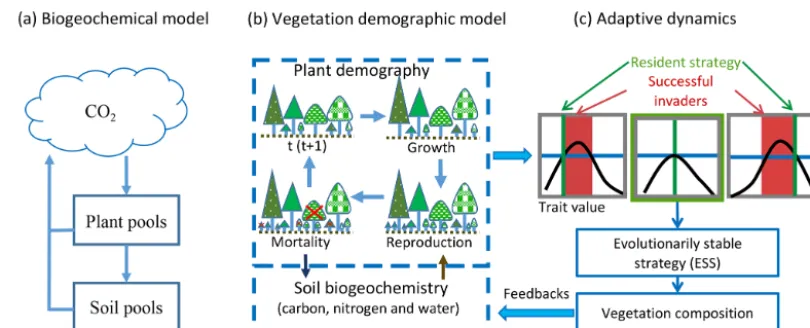
In current Earth system models (ESMs), the terrestrial car-bon cycle is usually simulated by pool-based compartment models that simulate ecosystem biogeochemical cycles as lumped pools and fluxes of plant tissues and soil organic mat-ter (Fig. 1a) (Emanuel and Killough, 1984; Eriksson, 1971; Parton et al., 1987; Randerson et al., 1997; Sitch et al., 2003). In these models, the dynamics of carbon can be described by a linear system of equations (Koven et al., 2015; Luo et al., 2001; Luo and Weng, 2011; Sierra and Mueller, 2015; Xia et al., 2013):

dX

dt =AX+BU, (1)

whereXis a vector of ecosystem carbon pools,Uis carbon input (i.e., gross primary production, GPP),B is the vector of allocation parameters to autotrophic respiration and plant carbon pools (e.g., leaves, stems and fine roots), andAis a matrix of carbon transfer and turnover. In this system, carbon dynamics are defined by carbon input (U), allocation (B), and residence time and transfer coefficients (A). The alloca-tion schemes (B) are thus embedded in a linear system, or quasi-linear system if the allocation parameters in B are a function of carbon input (U) or plant carbon pools (X).

The modeling of allocation in this system (i.e., the pa-rameters in vector B) is usually based on plant allometry, biomass partitioning and resource limitation (De Kauwe et al., 2014; Montané et al., 2017). The allocation parameters are either fixed ratios to leaves, stems and roots, which may vary among plant functional types (e.g., CENTURY, Parton et al., 1987; TEM, Raich et al., 1991; CASA, Randerson et al., 1997), or are responsive to climate and soil conditions as a way to phenomenologically mimic the shifts in allo-cation that are empirically observed or hypothesized (e.g., CTEM, Arora and Boer, 2005; ORCHIDEE, Krinner et al., 2005; LPJ, Sitch et al., 2003). These modeling approaches either assume that vegetation is equilibrated (fixed ratios) or average the responses of plant types to changes in environ-mental conditions as a collective behavior. Thus, the carbon dynamics in these models can be constrained by selecting ap-propriate parameters of allocation, turnover rates and transfer coefficients to fit the observations (Friend et al., 2007; Hoff-man et al., 2017; Keenan et al., 2013).

To predict transient changes in vegetation structure and composition in response to climate change, vegetation de-mographic models (VDMs) that are able to simulate tran-sient population dynamics are being incorporated into ESMs (Fisher et al., 2018; Scheiter and Higgins, 2009). Generally, VDMs explicitly simulate demographic processes, such as plant reproduction, growth and mortality, to generate the dy-namics of populations (Fig. 1b). To speed computations and minimize complexity, groups of individuals are usually

mod-eled as cohorts. With multiple cohorts and plant functional types (PFTs), VDMs can bring plant functional diversity and adaptive dynamics into the system when explicitly simulat-ing individual-based competition for different resources and vegetation succession and thus predict dominant plant trait changes with environmental conditions and ecosystem de-velopment (Scheiter et al., 2013; Scheiter and Higgins, 2009; Weng et al., 2015).

The combinations of plant traits represent the competition strategies at different stages of ecosystem development. Evo-lutionarily, a strategy that can outcompete all other strate-gies in the environment created by itself will be dominant. This strategy is called an evolutionarily stable strategy or a competitively optimal strategy (McGill and Brown, 2007). In VDMs, competitively optimal strategies can therefore be rea-sonably predicted based on the costs and benefits of different strategies (i.e., combinations of plant traits) through their ef-fects on demographic processes (i.e., fitness) and ecosystem biogeochemical cycles (Fig. 1c) (e.g., Farrior et al., 2015; Weng et al., 2015).

The dynamics of plant traits can substantially change pre-dictions of ecosystem biogeochemical dynamics since they change the key parameters of vegetation physiological pro-cesses and soil organic matter decomposition (e.g., Dybzin-ski et al., 2015; Farrior et al., 2015; Weng et al., 2017). There-fore, the key parameters that are used to estimate carbon dy-namics in the linear system model (Eq. 1), such as allocation (B) and residence times in different carbon pools (matrixA, which includes coefficients of carbon transfer and turnover time) become functions of competition strategies that vary with environment and carbon input. In addition, the turnover of vegetation carbon pools becomes a function of allocation, leaf longevity, fine root turnover and tree mortality rates, which change with vegetation succession and the most com-petitive plant traits. These changes make the system nonlin-ear and can lead to large biases within the framework of the compartmental pool-based models as represented by Eq. (1) (Sierra et al., 2017; Sierra and Mueller, 2015). Because of the high complexity associated with demographic and competi-tion processes, the model prediccompeti-tions are usually sensitive to the parameters in these processes and are of high uncertainty (e.g., Pappas et al., 2016).

con-Figure 1.Hierarchical structure of vegetation models.

centration [CO2] sheds light on the otherwise inscrutable processes leading to varied soil water dynamics in a land model coupled with an VDM (Weng et al., 2015). Recog-nizing the benefit, Weng et al. (2017) included both a simpli-fied analytical model and a more complicated VDM to under-stand competitively optimal leaf mass per area, competition between evergreen and deciduous plant functional types, and the resulting successional patterns.

In this study, we use a stand-alone simulator derived from the LM3-PPA model (Weng et al., 2017, 2015) to show how forests respond to elevated [CO2] and nitrogen availability via different competitively optimal allocation strategies. The demographic processes of this model have been coupled into the land model of the Geophysical Fluid Dynamical Labora-tory’s Earth System Model (Shevliakova et al., 2009; Weng et al., 2015) and are being added to NASA Goddard Institute for Space Study’s Earth system model, ModelE (Schmidt et al., 2014). Using this model, we simulate the shifts in com-petitively optimal allocation strategies in response to elevated [CO2] at different nitrogen levels based on insights from the analytical model derived by Dybzinski et al. (2015). Dy-bzinski et al. (2015)’s model predicts that increases in car-bon storage at elevated [CO2] relative to storage at ambient [CO2] are largely independent of total nitrogen because of an increasing shift in carbon allocation from long-lived, low-nitrogen wood to short-lived, high-low-nitrogen fine roots under elevated [CO2] with increasing nitrogen availability. Here, we analyze the simulated ecosystem carbon cycle variables (gross and net primary production, allocation, and biomass) of separate monoculture and polyculture model runs. In the monoculture runs, ecosystem properties are the result of the prescribed allocation strategies of a given PFT. In the poly-culture runs, competition between the different allocation strategies results in succession and the eventual dominance of the most competitive allocation strategy for a given ni-trogen availability and [CO2] level. Since everything else in the model is identical, we are able to compare the

predic-tions of single fixed strategies with competitively optimal al-location strategies by comparing the ecosystem properties of these two types of runs.

2 Methods and materials

2.1 BiomeE model overview

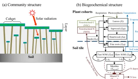
We used a stand-alone ecosystem simulator (Biome Eco-logical strategy simulator, BiomeE) to conduct simulation experiments. BiomeE is derived from the version of LM3-PPA used in Weng et al. (2017), and its code is available at Github (https://github.com/wengensheng/BiomeESS, last access: 27 November 2019). In this version, we simplified the processes of energy transfer and soil water dynamics of LM3-PPA (Weng et al., 2015) but still retained the key fea-tures of plant physiology and individual-based competition for light, soil water and, via the decomposition of soil or-ganic matter, nitrogen (Fig. 2 and Supplement I for details). In this model, individual trees are represented as sets of co-horts of similarly sized trees and are arranged in different vertical canopy layers according to their height and crown area following the rules of the perfect plasticity approxima-tion (PPA) model (Strigul et al., 2008). Sunlight is partiapproxima-tioned into these canopy layers according to Beer’s law. Thus, a key parameter for light competition, critical height, is defined; all the trees above this context-dependent height get full sunlight and all trees below this height are shaded by the upper-layer trees.

ni-Figure 2.Structure of BiomeE.(a)Vegetation structure: trees organize their crowns into canopy layers according to both their height and their crown area following the rules of the PPA model, which mechanistically models light competition.(b)Biogeochemical structure and compartmental pools. The green, brown and black lines are the flows of carbon, nitrogen, and coupled carbon and nitrogen, respectively. The green box is for carbon only. The brown boxes are nitrogen pools. The black boxes are for both carbon and nitrogen pools, whereXcan be C (carbon) and N (nitrogen). The C:N ratios of leaves, fine roots, seeds and microbes are fixed. The C:N ratios of woody tissues, fast soil organic matter (SOM) and slow SOM are flexible. Only one tree’s C and N pools are shown in this figure. The blue box and arrows are for water storage in soil and fluxes of rainfall, evaporation and transpiration. The model can have multiple cohorts of trees, which share the same pool structure. The dashed line separates the aboveground and belowground processes.

trogen pool for mineralized nitrogen in soil. The simula-tion of SOM decomposisimula-tion and nitrogen mineralizasimula-tion is based on the models of Gerber et al. (2010) and Manzoni et al. (2010) and described in detail in Weng et al. (2017). The decomposition rate of a SOM pool is determined by the basal turnover rate together with soil temperature and mois-ture. The nitrogen mineralization rate is a function of decom-position rate and the C:N ratio of the SOM. Microbes must consume more carbon in the high C:N ratio SOM pools to get enough nitrogen and must release excessive nitrogen in the low C:N ratio SOM pools to get enough carbon for en-ergy (Weng et al., 2017).

Plant growth and reproduction are driven by the carbon assimilation of leaves via photosynthesis, which is in turn dependent on water and nitrogen uptake by fine roots. The photosynthesis model is identical to that of LM3-PPA (Weng et al., 2015), which is a simplified version of Leuning model (Leuning et al., 1995). This model first calculates photosyn-thesis rate, stomatal conductance and water demand of the leaves of each tree (cohort) in the absence of soil water limi-tation. Then, it calculates available water supply as a func-tion of fine root surface area and soil water content. The demand-based assimilation rate and stomatal conductance

are adjusted if soil water supply is less than plant water de-mand. Soil water content is calculated based on the fluxes of precipitation, soil surface evaporation and plant water update (transpiration) in three layers of soil to a depth of 2 m (see Supplement I for details).

Assimilated carbon enters into the NSC pool and is subse-quently used for respiration, growth and reproduction. Em-pirical allometric equations relate woody biomass (including coarse roots, bole and branches), crown area and stem diame-ter. The individual-level dimensions of a tree, i.e., height (Z), biomass (S) and crown area (ACR), are given by empirical al-lometries (Dybzinski et al., 2011; Farrior et al., 2013):

Z (D)=αZDθZ,

S (D)=0.25π 3ρWαZD2+θZ,

ACR(D)=αcDθc, (2)

a PFT-specific taper constant, andρW is PFT-specific wood density (kg C m−3) (Table 1).

We set targets for leaf (L∗_{), fine root (FR}∗_{) and sapwood} cross-sectional area (A∗_SW) that govern plant allocation of nonstructural carbon and nitrogen during growth. These tar-gets are related by the following equations based on the as-sumption of the pipe model (Shinozaki et al., 1964):

L∗(D, p)=l∗·ACR(D)·σ·p(t ),

FR∗(D)=ϕRL·l∗·ACR(D)

γ ,

A∗_SW(D)=αCSA·l∗·ACR(D) , (3) whereL∗(D, p), FR∗(D)andA∗_SW(D)are the targets of leaf mass (kg C per tree), fine root biomass (kg C per tree) and sapwood cross-sectional area (m2/tree), respectively, at tree diameterD;l∗is the target leaf area per unit crown area of a given PFT;ACR(D)is the crown area of a tree with diameter D;σis PFT-specific leaf mass per unit area (LMA);p(t )is a PFT-specific function ranging from zero to one that governs leaf phenology (Weng et al., 2015);ϕRLis the target ratio of total root surface area to the total leaf area;γ is specific root area; andαCSAis an empirical constant (the ratio of sapwood cross-sectional area to target leaf area). The phenology func-tionp(t )takes values 0 (nongrowing season) or 1 (growing season) following the phenology model of LM3-PPA (Weng et al., 2015). The onset of a growing season is controlled by two variables, growing degree days (GDDs) and a weighted mean daily temperature (Tpheno), while the end of a growing season is controlled byTpheno(see Supplement I for details of the phenology model).

2.1.1 Nitrogen uptake

The rate of nitrogen uptake (U, g N m−2h−1) from the soil mineral nitrogen pool is an asymptotically increasing func-tion of fine root biomass density (CFR,total, kg C m−2), fol-lowing McMurtrie et al. (2012)

U=fU,max·Nmineral·

CFR,total CFR,total+KFR

, (4)

where Nmineral is the mineral nitrogen in soil (g N m−2), fU,maxis the maximum rate of nitrogen absorption per hour when CFR,total approaches infinity, andKFR is a shape pa-rameter (kg C m−2) at which the nitrogen uptake rate is half of the parameterfU,max. The nitrogen uptake rate of an indi-vidual tree (Utree, kg N h−1tree−1) is calculated as follows:

Utree=U·

CFR,tree CFR,total

, (5)

where,CFR,treeis the fine root biomass of a tree (kg C tree−1). The nitrogen absorbed by roots enters into the NSN pool and then is allocated to plant tissues through plant growth.

2.1.2 Allocation and plant growth

The partitioning of carbon and nitrogen into the plant pools (i.e., leaves, fine roots and sapwood) is limited by the allo-metric equations, targets of leaves, fine roots and sapwood cross-sectional area, and the stoichiometry (i.e., C:N ratios) of these plant tissues. At a daily time step, the model calcu-lates the amount of carbon and nitrogen that are available for growth according to the total NSC and NSN and current leaf and fine root biomass. Basically, the available NSC (GC) is the summation of a small fraction (f1) of the total NSC in an individual plant and the differences between the targets of leaf and fine roots and their current biomass capped by a larger fraction (f2) of NSC (Eq. 6a). The available NSN (GN) is analogous to that of the NSC and meets approximately the stoichiometrical requirement of plant tissues (Eq. 6b). GC=min(f1NSC+L∗+FR∗−L−FR, f2NSC), (6a) GN=min(f1NSN+N_L∗+N_FR∗ −NL−NFR, f2NSN),

(6b) whereL∗ and FR∗ are the targets of leaves and fine roots, respectively (see Eq. 3);Land FR are current leaf and fine roots biomass, respectively; andN_L∗andN_FR∗ are nitrogen of leaves and fine roots at their targets according to their tar-get C:N ratios. The parameterf1is the fraction of NSC (or NSN) for normal growth after leaves and fine roots approach their targets, andf2caps the maximum daily availability of NSC (or NSN) during the period of leaf flush at the begin-ning of a growing season. The parameterf1is much smaller thanf2. We letf1=1/(365×3)andf2=0.02 in this study. The allocation of the available NSC (i.e., GC) to wood (GW), leaves (GL), fine roots (GFR) and seeds (GF) fol-lows the equations below (Eq. 7). These equations describe the mass growth of plant tissues with nitrogen effects on the carbon allocation between high-nitrogen tissues and low-nitrogen tissues (wood) for maximizing leaves and fine roots growth (GLandGFR, respectively), optimizing carbon usage at given nitrogen supply (GN) and keeping the tissues at their target C:N ratios.

GC≥GW+GL+GFR+GF, (7a)

GN≥ GL CNL,0

+ GFR CNFR,0

+ GF CNF,0

+ GW CNW,0

, (7b)

(FR+GFR) γ (L+GL)/σ

=ϕRL, (7c)

GL+GFR=Min

L∗+FR∗−L−FR, fLFR,maxGC,

·rS/D, (7d)

GF=

GC−Min

L∗+FR∗−L−FR, fLFR,maxGC,

rS/D

,

·v·rS/D, (7e)

GW=

GC−Min

L∗+FR∗−L−FR, fLFR,maxGC,

rS/D

,

Table 1.Model parameters.

Symbol Definition Unit Default value Reference

αZ Parameter of tree height m m−0.5 36 Farrior et al. (2013)

θZ Diameter exponent of tree height – 0.5 Farrior et al. (2013)

3 Taper factor – 0.75 Weng et al. (2015)

ρW Wood density Kg C m−3 300 Jenkins et al. (2003)

αC Parameter of crown area m m−1.5 150 Farrior et al. (2013)

θC Diameter exponent of crown area – 1.5 Farrior et al. (2013)

l∗ Target crown leaf area layers (crown leaf area index)

m2m−2 3.5 –

σ Leaf mass per unit area kg C m−2 0.14 Wright et al. (2004)

γ Specific root area, calculated from root radius and density

m2kg C−1 34.5 Pregitzer et al. (2002)

φRL Ratio of target fine root area to target leaf area

m2m−2 Varied with PFTs –

αCSA Ratio of target sapwood cross-sectional area to target leaf area

m2m−2 0.2×10−4 McDowell et al. (2002)

fU,max Maximum mineral nitrogen absorption rate

h−1 0.5 –

KFR Root biomass at which the N-uptake rate is half of the maximum

kg C m−2 0.3 –

CNL,0 Target C:N ratio of leaves kg C kg N−1 76.5 (Function of LMA) Wright et al. (2004)

CNFR,0 Target C:N ratio of fine roots kg C kg N−1 60 Magill et al. (2004)

CNW,0 Target C:N ratio of wood kg C kg N−1 350 Martin et al. (2015)

CN_F,0 Target C:N ratio of seeds kg C kg N−1 20 Soriano et al. (2011)

f1 Supply rate of NSC and NSN at normal growth

– 1/(3·365) –

f2 Maximum fraction of NSC and NSN used for growth in a day

– 0.02 –

fLFR,max Maximum fraction of available carbon allocated to leaves and fine roots

– 0.85 –

v Fraction of carbon converted to seeds – 0.1 –

rD/S Nitrogen-limiting factor – Solved by the model (Eqs. 9 and 10) –

where CNL,0, CNFR,0, CNF,0, and CNW,0are the target C:N ratios of leaves, fine roots, seeds, and sapwood, respectively; γ is specific root area (m2kg C−1);σ is leaf mass per unit area (kg C m−2);fLFR,max is the maximum fraction of GC for leaves and fine roots (0.85 in this study); v is the frac-tion of left carbon for seeds (0.1 in this study); and rS/D is a nitrogen-limiting factor ranging from 0 (no nitrogen for leaves, fine roots and seeds) to 1 (nitrogen available for full growth of leaves, fine roots and seeds). The parameterrS/D controls the allocation ofGCandGNto the four plant pools (Eq. 7a). It can be analytically solved as follows (Eqs. 8 and 9).

rS/D=Min

1,Max

0,GN−GC/CNW N0_−G

C/CNW

, (8)

where N0 is defined as the potential nitrogen demand for plant growth atrS/D=1 (i.e., no nitrogen limitation),

N0≡ γ σ

FR+Min

L∗+FR∗−L−FR fLFR,maxGC

−ϕRLL

(γ σ+ϕRL)CNL

+ ϕRL

L+Min

L∗+FR∗−L−FR fLFR,maxGC

−γ σ L

(γ σ+ϕRL)CNFR

+ v

GC−Min

L∗+FR∗−L−FR, fLFR,maxGC

CNF

+ (1−v)

GC−Min

L∗+FR∗−L−FR fLFR,maxGC

CNW

,

rS/D=1). The excessive nitrogen (GN−N0) will be returned to the NSN pool (as if they were never taken out). When GC/CNW,0< GN< N0(i.e., 0< rS/D<1), allGCandGN will be used in new tissue growth; however, the leaves and fine roots cannot reach their targets at this step (i.e. they are down-regulated). WhenGN≤GC/CNW,0(rS/D=0), all the GN will be allocated to sapwood and the excessive carbon (GC−GNCNW,0) will be returned to NSC pool. This is a very rare case since a lowGN leads to low leaf growth, reducing GCbefore the caseGN< GC/CNW,0happens. Therefore, in most cases, Eq. (7a) isGC=GW+GL+GFR+GF. Over-all, this strategy down-regulates leaf production under low nitrogen conditions while making use of assimilated carbon in height-structured competition for light.

Allocation to wood tissues (GW) drives the growth of tree diameter, height and crown area and thus increases the targets of leaves and fine roots (Eq. 3). By differentiating the stem biomass allometry in Eq. (2) with respect to time, using the fact that dS/dt equals the carbon allocated for wood growth (GW), we have the diameter growth:

dD dt =

GW

0.25π 3ρwαz(2+θz)D1+θZ

, (10)

This equation transforms the mass growth to structural changes in tree architecture. With an updated tree diameter, we can calculate the new tree height and crown area using allometry equations (Eq. 2) and targets of leaf and fine root biomass (Eq. 3) for the next growth step.

Overall, this is a flexible allocation scheme and still fol-lows the major assumptions in the previous version of LM3-PPA (Weng et al., 2015, 2017). This allocation scheme pri-oritizes the allocation to leaves and fine roots, maintains a minimum growth rate of stems, and keeps the constant area ratio of fine roots to leaves. Based on these allocation rules, the average allocation of carbon and nitrogen to leaves, fine roots and wood over a growing season are governed by the targets for the leaf area per unit crown area (i.e., crown leaf area index, l∗) and fine root area per unit leaf area (ϕRL). Since the crown leaf area index, l∗, is fixed in this study, ϕRLis the key parameter determining the relative allocation of carbon to fine roots and stems. A highϕRLmeans a high relative allocation to fine roots and therefore low relative al-location to stems and vice versa. Note that hereφRLis fixed for each PFT and will remain so for all the model runs.

The process of choosing a context-dependent competi-tively dominantϕRLwill take place after finding the fitness of each ϕRLin monoculture and in competition with other PFTs (i.e., different values ofϕRL). The competitively opti-mal strategy is the one that can successfully exclude all oth-ers in the processes of competition and succession, but it is not necessarily the one that maximizes production in mono-culture. For example, each ϕRL creates an environment of light profile and soil nitrogen in its monoculture. OtherϕRL PFTs may have higher fitness in this environment than the

one that creates it. Only the competitively dominant strategy has the highest fitness in the environment it creates (Fig. 1c).

2.2 Site and data

Data pertaining to vegetation, climate and soil at Harvard Forest (Aber et al., 1993; Hibbs, 1983; Urbanski et al., 2007) were used to design the plant functional types (PFTs) and ecosystem nitrogen levels used in the simulation ex-periments, to drive the model and to calibrate model pa-rameters. Harvard Forest is located in Massachusetts, USA (42.54◦, −72.17◦). The climate of Harvard Forest is cool temperate with an annual precipitation of 1050 mm, dis-tributed fairly evenly throughout the year. The annual mean temperature is 8.5◦C with a high monthly mean tempera-ture of 20◦C in July and a low of −7◦C in January. The soils are mainly sandy loam with an average depth of around 1 m and are moderately well drained in most areas. In for-est sites, soil carbon is around 8 kg C m−2 and nitrogen 300 g N m−2(Compton and Boone, 2000). The vegetation is deciduous broadleaf (mixed) forest with its major species be-ing red oak (Quercus rubra), red maple (Acer rubrum), black birch (Betula lenta), white pine (Pinus strobus) and hem-lock (Tsuga canadensis) (Compton and Boone, 2000; Sav-age et al., 2013). The data used to drive our model runs are gap-filled hourly meteorological data at Harvard Forest from 1991 to 2006, obtained from North American Carbon Pro-gram (NACP) site-level synthesis datasets (Barr et al., 2013).

2.3 Simulation experiments

We set two atmospheric CO2concentration ([CO2]) levels, 380 and 580 ppm, and eight ecosystem total nitrogen lev-els (ranging from 114.5 to 552 g N m−2 at the interval of 62.5 g N m−2) by assigning the initial content of the slow SOM pool for our simulation experiments (Table 2). This range covers the soil nitrogen contents across the plots at Harvard Forest with different species compositions and land-use history (200–300 g N m−2) (Compton and Boone, 2000; Melillo et al., 2011) and represents the range from infertile to fertile soils in temperate forests (Post et al., 1985; Yang et al., 2011). The nitrogen cycles through the plant and soil pools and is redistributed among them via plant demographic processes, soil carbon transfers and plant uptake. In all the simulation experiments, we assume the ecosystem has no ni-trogen inputs and no outputs for convenience since we al-ready have eight total nitrogen levels to represent the conse-quences of different nitrogen input and output processes at an equilibrium state. The PFTs were based on an evergreen needle-leaved tree PFT with different leaf to fine root area ratios,ϕRL, in the range from 1 to 8 (Table 2). Simply stated, the PFTs we investigate only differ in parameterϕRL.

Table 2.Simulation experiments.

Type Model runs Initial PFT(s)

ϕRL

Ecosystem total nitro-gen levels

CO2concentration [CO2]

Monoculture runs One model run per combination of PFT (ϕRL), nitrogen level and CO₂concentration.

One of the following PFTs:ϕRL=1, 2, 3, 4, 5, 6, 7 or 8.

Eight levels rang-ing from 114.5 to 552 g N m−2 at the in-terval of 62.5 g N m−2: (i.e., 114.5, 177, 239.5, 302, 364.5, 427, 489.5 and 552 g N m−2)

Ambient: 380 ppm Elevated: 580 ppm

Polyculture run I One model run per combination of nitro-gen level and CO2 concentration.

All the PFTs (ϕRL=1– 8) used in the monocul-ture runs.

Polyculture run II One model run per combination of nitro-gen level and CO₂ concentration.

Eight PFTs with ϕRL ranging from 4.5–0.5i to 8.5–0.5i at the in-terval of 0.5, where i denotes the eight nitro-gen levels from 114.5 to 552 g N m−2.

ecosystem nitrogen availability. The model runs started with multiple PFTs are called “polyculture runs” (eight PFTs with differentϕRLat the beginning, although many are driven to extinction during a given model run). We conducted one set of monoculture runs and two sets of polyculture runs (Ta-ble 2).

In the monoculture runs, we run the full combinations of eight PFTs with root/leaf area ratios (ϕRL)from 1 to 8, eight ecosystem total nitrogen levels and two CO2concentrations (380 and 580 ppm) (Table 2). For the eight PFTs, only those withϕRL≤6 survived at ambient [CO2] (380 ppm) because the carbon assimilated by leaves could not meet the demand by plant tissues at ϕRL>6. The monoculture runs are for exploring the model predictions of gross primary produc-tion (GPP), net primary producproduc-tion (NPP), and allocaproduc-tion and biomass at equilibrium with fixedϕRLat different total nitro-gen levels.

In polyculture run I, we used the same PFTs as in those monoculture runs, where their ϕRL varied from 1 to 8 at the interval of 1.0 and the ecosystem total nitrogen levels were the same as those used in the monoculture runs (Ta-ble 2). This set of polyculture runs was used to explore suc-cessional patterns at both ambient and elevated [CO2] (380 and 580 ppm, respectively). However, this set of model runs could not show the details of equilibrium plant biomass and allocation patterns along the nitrogen gradient because of the large intervals between theϕRLvalues.

To achieve greater resolution in our competition predic-tions, we designed the polyculture run II using a dynamic PFT combination scheme, according to the ranges of ϕRL obtained from the polyculture run I that could survive at a particular nitrogen level at both CO2 concentrations. For each nitrogen level, we set eight PFTs with ϕRL that

var-ied in a range 3.5 (e.g.,x∼x+3.5) at the interval of 0.5, starting with the highest ϕRL of 8.0 at the lowest N level (114.5 g N m−2) and decreasing 0.5 per level of increase in ecosystem total N. We used i=1, 2, . . . , 8 to denote the eight N levels from 114.5 to 552 g N m−2. TheϕRL of the eight PFTs at each level were 5.0–0.5i, 5.5–0.5i, . . . , 8.5– 0.5i(Table 2). For example, at the nitrogen of 114.5 g N m−2 (i=1), theϕRLof the eight PFTs were 4.5, 5.0, . . . , 8.0 and at 177 g N m−2(i=2) they were 4.0, 4.5, . . . , 7.5.

For both monoculture and polyculture runs, visual in-spection indicated that stands had reached equilibrium af-ter∼1200 years. To be conservative, we present equilibrium data by averaging model properties between years 1400 and 1800. We compared simulated equilibrium GPP, NPP, allo-cation (both absolute amount of carbon and fractions of the total NPP) and plant biomass of the polyculture run II with those from the monoculture runs. We used the results from one PFT (ϕRL=4) to highlight the differences of plant re-sponses with competitively optimal allocation strategies ob-tained from the polyculture run II.

3 Results

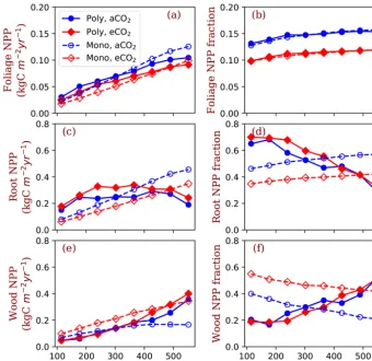
Figure 3.GPP, NPP, allocation and plant biomass at equilibrium state simulated by monoculture runs. GPP: gross primary production; NPP: net primary production;fNPP,x: the fraction of NPP allocated tox, wherexis root (fine roots), leaf (leaves in crown) or wood (including tree trunk, stems and coarse roots). The data are from the averages of the model run years from 1400 and 1800. Each model run is initiated with one PFT with a fixed ratio of fine root area to leaf area (ϕRL).

ofϕRL, allocation of NPP to fine roots increases withϕRLin monoculture runs (Fig. 3c). As a consequence, allocation of NPP to wood decreases as ϕRLincreases (Fig. 3d). Alloca-tion to leaves does not change much withϕRL(Fig. 3e, note differences in scale). Correspondingly, plant biomass at equi-librium decreases withϕRL(Fig. 3f). The effects of nitrogen on the allocation of carbon to fine roots and wood follow our allocation model assumptions because more carbon is allo-cated to low-nitrogen woody tissues in our model when ni-trogen is limited. However, the amplitude of changes in GPP and NPP induced by nitrogen availability is lower than the amplitude of changes resulting from different values ofϕRL in the monoculture runs.

We used two sets of polyculture runs to look for theϕRL that is closest to competitively optimal. In the polyculture run I, where ϕRL ranges from 1 to 8 at all nitrogen levels, the winning strategy (ϕRL) increases from 5 to 2 as the total nitrogen increases from 114.5 to 489.5 g N m−2at ambient [CO2] (380 ppm) (Fig. 4a, c, g, e). Elevated [CO2] (580 ppm) shifts the winning strategy to higher (ϕRL) at all the total ni-trogen levels. As shown in Fig. 4, the winning strategy shifts

fromϕRL=5 toϕRL=8 at 114.5 g N m−2and fromϕRL=2 toϕRL=4 at 489.5 g N m−2. In some situations (e.g., Fig. 4g and Figs. S2 and S3), it takes a long time for the most com-petitive PFTs to out-compete the previously dominant PFTs because of the sequential replacement of dominant PFTs dur-ing the course of succession and the slow growth rate of trees in understory.

polycul-Figure 4.Successional patterns of polyculture run I at ambient and elevated [CO2] concentrations.ϕRLis the fixed ratio of fine root area to leaf area of a particular strategy.

ture runs (Fig. 5d). Also, the dependence of NPP:GPP ratio on nitrogen is higher in the polyculture runs than it is in the monoculture runs (Fig. 5c).

Allocation of NPP to leaves increases with nitrogen in all conditions, i.e. both competition and monoculture at both ambient [CO2] and elevated [CO2] (Fig. 6a). Foliage NPP is similar in these four model runs when nitrogen is low. At high nitrogen (>400 g N m−2), polyculture runs have higher foliage NPP than the monoculture runs generally. Allocation to leaves is relatively stable across the nitrogen gradient at the two [CO2] levels (Fig. 6b). The fraction of NPP allocated to leaves changes little with nitrogen (Fig. 6b) and it is uni-versally higher at ambient [CO2] than it is at elevated [CO2]. Fine root NPP does not significantly change with ecosys-tem total nitrogen in polyculture runs, whereas it increases monotonically with increasing nitrogen in monoculture runs (Fig. 6c). Elevated [CO2] increases fine root allocation at low nitrogen in polyculture runs but decreases root alloca-tion irrespective of nitrogen in monoculture runs (Fig. 6c). The fraction of NPP allocated to fine roots decreases with ni-trogen at both CO2concentrations in polyculture runs, but it increases slightly in monoculture runs (Fig. 6d). In mono-culture runs, elevated [CO2] reduces the fraction of NPP

allocated to fine roots at all nitrogen levels. In polyculture runs, fractional allocation to fine roots increases at elevated [CO2] when nitrogen is low (e.g., 114.5–302 g N m−2) and decreases at elevated [CO2] when nitrogen is high (e.g., 364– 552 g N m−2).

In the reverse of the fine root response, NPP allocation to woody tissues increases with total nitrogen in both compe-tition and monoculture runs (Fig. 6e). In polyculture runs, the fraction of allocation to woody tissues decreases at ele-vated [CO2] when ecosystem total nitrogen is low (e.g., 114– 245 g N m−2) and increases at elevated [CO2] when ecosys-tem total nitrogen is high (e.g., 302–552 g N m−2).

Figure 5.Winning PFTs (ϕRL,a) in polyculture run II and equilibrium gross primary production (GPP,b), net primary production (NPP,c) and carbon use efficiency (NPP/GPP,d) at two CO2concentrations (aCO2: 380 ppm;eCO2: 580 ppm). The closed symbols with solid lines represent polyculture runs. The open symbols with dashed lines represent monoculture runs (onlyϕRL=4 shown in this figure).ϕRLis the fixed ratio of fine root area to leaf area of a particular strategy.

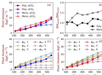
which amplifies plant biomass responses to elevated [CO2] with increasing nitrogen (Fig. 7c and d).

4 Discussion

Our simulations show that the predicted responses of individ-ual plants to elevated [CO2] can be significantly changed by explicit inclusion of competition processes. Here, the major tradeoff for light- and N-limited trees is the relative alloca-tion between stems and fine roots (Dybzinski et al., 2011). Although the wood allocation (and thus carbon sequestration potential) of every PFT used in this study increases under ele-vated [CO2] at all nitrogen levels (e.g., Fig. 6e, dashed lines), only those PFTs that allocate more to fine roots (with lower carbon sequestration potential) can survive competition un-der elevated [CO2] (Fig. 6c, solid lines). Put together, explicit inclusion of competition processes reduces the expected in-crease in biomass (and thus carbon sequestration potential) under elevated [CO2] compared with simulations that do not include competition processes (Fig. 7b).

Since there is a lack of direct observations or experiments to quantitatively validate the long-term patterns predicted by our model, we did not calibrate it to fit observations at Har-vard Forest. In the following section, we analyze the model processes in detail and validate our modeling approach by comparing the general patterns from observations and exper-iments with model predictions. These comparisons also shed

light on the modeling of allocation and vegetation responses to elevated [CO2].

4.1 Mechanisms of game-theoretic allocation modeling and simulation results validation

Figure 6.Allocation to leaves, fine roots and wood tissues of the competition and monoculture runs at the eight total nitrogen levels and two CO2concentrations (aCO2: 380 ppm;eCO2: 580 ppm). Panels(a),(c)and(e)show the NPP allocated to the tissues and panels(b),(d)and (f)show the fractions of the allocation in total NPP. The closed symbols with solid lines represent polyculture runs (Poly). The open symbols with dashed lines represent monoculture runs (onlyϕRL=4 is shown in this figure, Mono).ϕRLis the fixed ratio of fine root area to leaf area of a particular strategy.

new wood tissues must be continuously produced (especially early in the growing season) to maintain the functions of tree trunks and branches (Cuny et al., 2012; Michelot et al., 2012; Plomion et al., 2001). This parameter does not change the fact that leaves and fine roots are the priority in allocation, since allocation ratios to stems are around 0.4–0.7 in tem-perate forests (Curtis et al., 2002; Litton et al., 2007). With a value of 0.85, parameterfLFR,maxseldom affects the over-all carbon over-allocation ratios of leaves, fine roots and stems. If fLFR,max=1 (i.e., the highest priority for leaf and fine root growth), simulated trunk radial growth would have un-reasonably high interannual variation because leaf and fine root growth would use all carbon to approach to their targets, leaving nothing for stems in some years of low productivity. The simulation of competition for light and soil resources is based on two fundamental mechanisms: (1) competition for light is based on the height of trees according to the PPA model, which assumes trees have perfectly plastic crown to capture light via stem (trunk) and branch phototropism

Figure 7.Plant biomass responses to elevated [CO2] and nitrogen. Panel(a)shows the equilibrium plant biomass (means of simulated plant biomass from model run year 1400 to 1800) in polyculture runs and monoculture runs (onlyϕRL=4 is shown as an example). Panel(b) shows the ratio of simulated plant biomass at elevated [CO2] to ambient [CO2] for both competition and monoculture runs. Panels(c)and (d)show the comparisons with monoculture runs withϕRLincreasing from 1 to 6 at ambient(c)and elevated [CO2](d). The closed symbols with solid lines represent polyculture runs. The open symbols with dashed lines represent monoculture runs (ϕRLranges from 1 to 6).ϕRL is the fixed ratio of fine root area to leaf area of a particular strategy.aCO2: 380 ppm;eCO2: 580 ppm.

the mechanism in our model) (e.g., Douma et al., 2012), but it may also occur through adaptive plastic responses or in-place subpopulation evolution of ecotypes (Grams and Andersen, 2007; McNickle and Dybzinski, 2013; Smith et al., 2013).

Generally, the predictions from competitively optimal al-location strategies predicted by our model can be found in large-scale forest censuses and site-level experiments, such as that (1) high-nitrogen environments (i.e., productive envi-ronments) favor high wood allocation and low root allocation (Litton et al., 2003; Poorter et al., 2012), (2) elevated [CO2] increases root allocation (Drake et al., 2011; Iversen, 2010; Jackson et al., 2009; Nie et al., 2013; Smith et al., 2013), (3) low nitrogen availability limits vegetation biomass re-sponses to elevated [CO2] as a result of high root allocation or root exudation (Jiang et al., 2019a; Norby and Zak, 2011), and (4) increases in vegetation biomass at elevated [CO2] are largely due to high wood allocation (Norby and Zak, 2011; Walker et al., 2019). These predictions emerge from the fun-damental assumptions of our model without tuning parame-ters to fit the data, providing some confidence in the robust-ness of our approach.

The literature on experimental responses of plant commu-nity to elevated [CO2] shows that the responses vary with site characteristics, forest composition, stand age, plant physio-logical responses and soil microbial feedbacks (Norby and

Zak, 2011; Terrer et al., 2016, 2018). For example, in the Duke Free Air CO2Enhancement (FACE) experiment, where the major trees are loblolly pine (Pinus taeda), increases in root production at elevated [CO2] stimulated increased nitro-gen supply that allowed the forest to sustain higher produc-tivity (Drake et al., 2011). However, in the Oak Ridge FACE, where the major trees are sweetgum (Liquidambar styraci-flua), increased fine-root production under elevated [CO2] did not result in increased net nitrogen mineralization and increases in root production declined after 8 years of CO2 enhancement (Iversen, 2010; Norby and Zak, 2011). In Euc-FACE (Jiang et al., 2019a), where the major trees are Euca-lyptus tereticornisand the soil is infertile, trees significantly increased their root exudation under limited nutrient supplies but had no significant increase in biomass in response to el-evated [CO2]. The BangorFACE experiment (Smith et al., 2013) found that interspecific competition (Alnus glutinosa,

in closed-canopy forests is not responsive to elevated [CO2] (Norby et al., 2003; Norby and Zak, 2011).

The nature of developing a model with generic assump-tions and balanced processes reduces its capability to predict all of these responses. For example, plants have a variety of physiological mechanisms to deal with excessive carbon sup-ply when plant demand (i.e., “sink”) is relatively low (Fatichi et al., 2019; Körner, 2006), such as down-regulating leaf photosynthesis rate by the accumulated assimilates (Gold-schmidt and Huber, 1992) or respiring excessive carbohy-drates to regenerate substrates for photosynthesis (Atkin and Macherel, 2009). But these mechanisms are short-term phys-iological responses (minutes to hours, sometimes days) for plants in situations of temporary nitrogen shortage, high ir-radiation or drought stress. It is not “economically” sustain-able in an infertile environment to maintain highly produc-tive leaves but often suppress their photosynthesis or respire a large portion of their assimilated carbon.

Root exudation is a critical process for plants. It can stim-ulate soil organic matter decomposition and nitrogen min-eralization to facilitate soil nitrogen supply at the expense of carbon (Cheng, 2009; Cheng et al., 2014; Drake et al., 2011; Phillips et al., 2011). The process of root exudation has been adopted by many models to couple with microbial pro-cesses in the determination of soil organic matter decompo-sition (Sulman et al., 2014; Wieder et al., 2014, 2015). Some carbon-only models, e.g., LM3 (Shevliakova et al., 2009), the parent model of this one, and TECO (Luo et al., 2001), incorporate root exudation to put extra carbon into the soil in order to avoid down-regulating canopy photosynthesis or overestimating vegetation biomass, both of which had been tuned against data. However, in a demographic competition model like this one, individual plants cannot reap a reward from root exudation as they do in nature when the microbial activities are not fully coupled and the nitrogen in soil is as-sumed fully accessible by roots of all individuals. Therefore, root exudation is not a competitive strategy in the system de-fined by the assumptions of this model.

Since the purpose of this study is to explore long-term eco-logical strategies in different but relatively stable environ-ments, we did not include these processes, especially since they present additional challenges in balancing the complex-ity of the tradeoffs between modeled demographic processes and plant traits. However, the lack of these processes does limit the predictions of instantaneous responses to variation in environmental conditions or resource supply and possibly of some long-term vegetation characteristics as well. For ex-ample, our model predicts reduced LAI under nitrogen limi-tation (Fig. S7) based on first principles, but it is incidentally the only mechanism that reduces the whole-canopy photo-synthesis rate in our model. There are mechanisms that in-crease nitrogen use efficiency at the expense of carbon by increasing LMA and therefore leaf longevity to maintain high LAI and high canopy-level photosynthesis rates (Aerts, 1995, 1999; Aerts and Chapin, 1999; Givnish, 2002). We did

not include these mechanisms in our simulations, although they are well developed in this model (Weng et al., 2017), because we wished to focus on the strategy of allocation. The clear descriptions of our model’s assumptions, its trace-able processes, and inclusion of the tradeoffs involved in aboveground and belowground competition provide a use-ful benchmark from which to incorporate additional mecha-nisms and tradeoffs.

4.2 Root over-proliferation vs. wood allocation

The allocation strategy that maximizes site vegetation biomass allocates very little to fine roots (Figs. 3 and S1). In contrast, the competitively optimal strategy allocates more carbon to fine roots, termed “fine-root over-proliferation” in the literature (Gersani et al., 2001; McNickle and Dybzin-ski, 2013; O’Brien et al., 2005). It is the result of a com-petitive “arms race”: while increasing fine root area under elevated [CO2] does not result in more nitrogen for an indi-vidual, failing to do so would cede some of that individual’s nitrogen to its neighbors. Because most nitrogen uptake is via mass flow and diffusion (Oyewole et al., 2017) and because both of these mechanisms depend on sink strength, individu-als with relatively greater fine root mass than their neighbors take a greater share of nitrogen, as was recently demonstrated empirically (Dybzinski et al., 2019; Kulmatiski et al., 2017). Thus, fine roots may over-proliferate for competitive reasons relative to lower optimal fine root mass in the hypothetical absence of an evolutionary history of competition (Craine, 2006; McNickle and Dybzinski, 2013). This may also ex-plain why root C:N ratio is highly variable (Dybzinski et al., 2015; Luo et al., 2006; Nie et al., 2013): a high density of fine roots in soil may be more important than the high ab-sorption ability of a single root in competing for soil nitrogen in the usually low mineral nitrogen soils.

commu-nity nitrogen uptake rate was independent of fine root mass in seedlings of numerous species, suggesting a high degree of fixed fine root over-proliferation. To improve root com-petition models, more detailed experiments that control root growth should be conducted to quantify the marginal bene-fits of roots in isolated, monoculture and polyculture envi-ronments.

At high soil nitrogen, height-structured competition for light (also a game-theoretic response, Falster and Westoby, 2003; Givnish, 1982) prevails and trees with greater relative allocation to trunks prevail. The balance between these two competitive priorities (fine roots vs. stems) can be observed in our model predictions as a shift from fine root allocation to wood allocation as soil nitrogen increases. The increases in the critical height (i.e. the context-dependent height of the shortest tree in canopy layer in the PPA) from low nitrogen to high nitrogen indicates a shift from the importance of com-petition for soil nitrogen to the importance of comcom-petition for light as ecosystem nitrogen increases (Fig. S8). Because the most competitive type shifts from high fine root allocation to low fine root allocation as ecosystem total nitrogen increases, increases in NPP and plant biomass across the nitrogen gra-dient are greater than the increases in NPP and plant biomass assuming allocation strategies in the absence of competition (Fig. 3). This greatly reduces the carbon cost of belowground competition as ecosystem total nitrogen increases. The de-crease in the fraction of NPP allocated to leaves at elevated [CO2] (Fig. 6b) occurs because of increases in total NPP and nearly constant absolute NPP allocation to foliage (Fig. 6a).

4.3 Model complexity and uncertainty

Compared with the conventional pool-based vegetation mod-els that use pools and fluxes to represent plant demographic processes at a land simulation unit (e.g., grid or patch), VDMs add two more layers of complexity. The first is the inclusion of stochastic birth and mortality processes of in-dividuals (i.e., demographic processes). These processes al-low the models to predict population dynamics and transient vegetation structure, such as size-structured distribution and crown organization (e.g., Moorcroft et al., 2001; Strigul et al., 2008). With changes in vegetation structure, allocation and mortality rates can change, generating a different carbon storage accumulation curve compared with those predicted by pool-based models where vegetation structure is not ex-plicitly represented (e.g., Weng et al., 2015). The second is the simulated shift in dominant plant traits during succession due to the shifting of competitive outcomes among different PFTs, which changes the allocation between fast- and slow-turnover pools and thus the parameters of allocation and the residence time of carbon in the ecosystem.

Together, these mechanisms may alter long-term predic-tions of the terrestrial carbon cycle due to changes in PFT-based parameters (Dybzinski et al., 2011; Farrior et al., 2013; Weng et al., 2015). As described in the Introduction, current

pool-based models can be described by a linear system of equations characterized by the key parameters of allocation, residence time and transfer coefficients (Eq. 1) with the rigid assumption of unchangeable plant types (Luo et al., 2012; Xia et al., 2013). In VDMs, however, allocation, residence time, leaf traits, phenology, mortality, plant forms and their responses to climate change are all strategies of competition whose success varies with the environmental conditions and the traits of the individuals they are competing against.

Many tradeoffs between plant traits can shift in response to environmental and biotic changes, limiting the applicabil-ity of varying a single trait, as we have in this study. For example, allocation, leaf traits, mycorrhizal types and nitro-gen fixation can all change with ecosystem nitronitro-gen avail-ability (Menge et al., 2017; Ordoñez et al., 2009; Phillips et al., 2013; Vitousek et al., 2013). The unrealistic effects of model simplification can be corrected by adding important tradeoffs that are missing. For example, the positive feedback between root allocation and SOM decomposition plays a role in mitigating the effects of tragedies of the commons of root over-proliferation (e.g., Gersani et al., 2001; Zea-Cabrera et al., 2006). High root allocation increases the decomposition rate of SOM and the supply of mineral nitrogen because of the high turnover rate of root litter, which favors a strategy of high wood allocation and reduces the competitive optimal fine root allocation. This negative feedback indicates that the model structure is flexible and that we can incorporate cor-rect mechanisms step by step to improve model prediction skills. Testing single strategies is still a necessary step to im-proving our understanding of the system and prediction skills of the models, though it could lead to unrealistic responses sometimes.

Dybzinski et al. (2015) predicts increasing fine root nitrogen concentration with increasing nitrogen availability. As a re-sult, there is less nitrogen to allocate to wood as nitrogen in-creases in the model of Dybzinski et al. (2015) than there is in the model presented here. These countervailing factors even out the ratio of plant biomass under elevated [CO2] relative to plant biomass under ambient [CO2] across the nitrogen gra-dient in Dybzinski et al. (2015), whereas their absence ampli-fies this ratio with increasing nitrogen in the model presented here. Our ability to diagnose and understand this discrepancy highlights the utility of deploying closely related analytical and simulation models (Weng et al., 2017).

We conducted simulations only at one site for the purpose of exploring the general patterns of competitively optimal allocation strategies and their responses to elevated [CO2] at different nitrogen availabilities. We can speculate about shifts in the competitively optimal allocation strategy in dif-ferent forest biomes by considering the effects of temperature on soil nitrogen supply via the SOM’s decomposition rate and its positive effect on net nitrogen mineralization. For ex-ample, the SOM decomposition rate is usually high in warm regions and low in cold regions (Davidson and Janssens, 2006) assuming there are no water limitations and SOM is equilibrated with carbon input. According to our model, allo-cation to roots is high in low nitrogen supply conditions (cold regions) and low in high nitrogen supply conditions (warm regions). This pattern can be found from temperate to boreal forest zones (Cairns et al., 1997; Gower et al., 2001; Reich et al., 2014; Zadworny et al., 2016). Temperature also alters NPP, i.e., carbon supply: as temperature goes down, NPP de-creases and nitrogen demand dede-creases, alleviating nitrogen limitation and leading to shifts of allocation to stems. There-fore, the differences in temperature effects on photosynthe-sis and SOM decomposition will determine competitive al-location strategy. Since SOM decomposition is more sensi-tive to temperature than gross primary production is at long-temporal and large spatial scales (Beer et al., 2010; Carey et al., 2016; Crowther et al., 2016), our model suggests that al-location will shift to wood in a warming world. Whether the carbon stored in that wood is enough to offset the carbon re-leased from increasing soil respiration is a critical question.

Water is also a critical factor affecting allocation and its responses to elevated [CO2]. Low soil moisture usually leads to high allocation to roots (Poorter et al., 2012). Elevated CO2can reduce transpiration (as found in our study as well, Figs. S9–S11) and therefore increase soil moisture, resulting in increases in allocation to stems and aboveground biomass (Walker et al., 2019). A game-theoretic modeling study us-ing the PPA framework shows that the competitively optimal allocation strategy shifts to high wood allocation at elevated [CO2] in environments with water limitation (Farrior et al., 2015). This is the opposite of the elevated [CO2] effects on allocation in nitrogen-limited environments as simulated in this study. According to field experiments, fine root alloca-tion is more responsive to nitrogen changes than it is to soil

moisture changes (Canham et al., 1996; Poorter et al., 2012). Poorter et al. (2012) attribute the mechanisms to the opti-mal strategies in response to the relative stable nitrogen sup-ply and stochastic water input in soil. The vertical distribu-tion of roots and the contribudistribu-tions of roots in different layers to water and nitrogen uptake also suggest that the uptake of soil nutrients are dominant in shaping root system architec-ture (Chapman et al., 2012; Morris et al., 2017), though root growth and turnover are flexible and sensitive to nitrogen and water supply (Deak and Malamy, 2005; Linkohr et al., 2002; Pregitzer et al., 1993).

4.4 Common principles for allocation modeling and implications

As shown in model intercomparison studies, the mechanisms of modeling allocation differ very much, leading to high vari-ation in their predictions (e.g., De Kauwe et al., 2014). Cali-brating model parameters to fit data may not increase model predictive skill because data are often also highly variable. Franklin et al. (2012) suggest that in order to build real-istic and predictive allocation models, we should correctly identify and implement fundamental principles. Our model predicts similar patterns to those predicted by the model of Valentine and Mäkelä (2012), which has very different pro-cesses of plant growth and allocation. However, these two models share fundamental principles, including (1) evolu-tionary or competitive optimization, (2) capped leaves and fine roots at given tree sizes, (3) structurally unlimited stem allocation (i.e., optimizing carbon use) because the woody tissues can serve as unlimited sink for surplus carbon, and (4) height–structure competition for light and root-mass-based competition for soil resources. Principles 2 and 3 are commonly used in models (De Kauwe et al., 2014; Jiang et al., 2019b). However, the different rules of implementing them (e.g., allometric equation, functional relationships, etc.) lead to highly varied predictions (as shown in De Kauwe et al., 2014), though model formulations may be very similar.

veg-etation properties and environmental conditions. With these first principles, the models can produce reasonable predic-tions, though the details of physiological and demographic processes vary among models.

For vegetation models designed to predict the effects of climate change, the important operational distinction is that the fundamental rules cannot or will not change as climate changes. Nor, presumably, will the underlying ecological and evolutionary processes change as climate changes. The emer-gent properties can change as climate changes, however, and the models built on the “scale-appropriate” unbreakable con-straints and ecological and evolutionary processes will be able to accurately predict changes in emergent ecosystem properties (Weng et al., 2017). In our opinion, the scientific effort to build better models is better served by understand-ing unrealistic predictions than by “fixunderstand-ing” them with unre-liable mechanisms when there is a lack of data or theory to make them consistent with observations. Validating assump-tions and initial responses are critical, and the long-term re-sponses can be validated via spatial patterns.

This modeling approach also demands improvement in model validation and benchmarking systems (Collier et al., 2018; Hoffman et al., 2017). As shown in this study, alloca-tion responses to elevated CO2at different nitrogen levels in monoculture runs are opposite to those in competitive alloca-tion runs. For example, in monoculture runs, elevated [CO2] increases wood allocation and decreases fine root allocation at low nitrogen; whereas in competitive allocation runs ele-vated [CO2] leads to low wood allocation and high fine root allocation. Simply calibrating our model against short-term observational data may improve the agreement with obser-vations but would not change the model’s predictions be-cause the model’s predictions emerge from its fundamental assumptions.

5 Conclusions

Our study illustrates that including the competition processes for light and soil resources in a game-theoretic vegetation de-mographic model can substantially change the prediction of the contribution of ecosystems to the global carbon cycle. Al-lowing the model to explicitly track the competitive alloca-tion strategies can generate significantly different ecosystem-level predictions (e.g., biomass and ecosystem carbon stor-age) than those of strategies in the absence of explicit com-petition. Building such a model requires differentiating be-tween the unbreakable tradeoffs of plant traits and ecolog-ical processes from the emergent properties of ecosystems. Drawing on insights from closely related analytical models to develop and understand more complicated simulation models seems, to us, indispensable. Evaluating these models also re-quires an updated model benchmarking system that includes the metrics of competitive plant traits during the development of ecosystems and their responses to global change factors.

Code and data availability. The model codes, simulated data and Python scripts used in this study are available from Github (https://github.com/wengensheng/BiomeE-Allocation, last access: 27 November 2019).

Supplement. The supplement related to this article is available on-line at: https://doi.org/10.5194/bg-16-4577-2019-supplement.

Author contributions. All authors contributed to model design, re-sults explanation and manuscript writing. EW and RD initially de-signed the simulation experiments. EW coded the model and imple-mented model runs and data analysis.

Competing interests. The authors declare that they have no conflict of interest.

Acknowledgements. The authors thank Benjamin Stocker, Mar-tin De Kauwe and other two anonymous referees for their insight-ful comments that greatly improved this paper. We also thank the USDA Forest Service Northern Research Station, Carbon Mitiga-tion Initiative at Princeton University, and the University of Texas at Austin for their support. Earth system modeling at GISS is sup-ported by the NASA Modeling, Analysis, and Prediction Program, and resources supporting this work were provided by the NASA High-End Computing Program through the NASA Center for Cli-mate Simulation (NCCS) at Goddard Space Flight Center.

Financial support. This research has been supported by the NASA Modeling, Analysis, and Prediction Program.

Review statement. This paper was edited by Sönke Zaehle and re-viewed by Benjamin Stocker, Martin De Kauwe and two anony-mous referees.

References

Aber, J. D., Magill, A., Boone, R., Melillo, J. M., and Steudler, P.: Plant and Soil Responses to Chronic Nitrogen Additions at the Harvard Forest, Massachusetts, Ecol. Appl., 3, 156–166, https://doi.org/10.2307/1941798, 1993.

Aerts, R.: The advantages of being evergreen, Trends Ecol. Evol., 10, 402–407, https://doi.org/10.1016/S0169-5347(00)89156-9, 1995.

Aerts, R.: Interspecific competition in natural plant communities: mechanisms, trade-offs and plant-soil feedbacks, J. Exp. Bot., 50, 29–37, https://doi.org/10.1093/jxb/50.330.29, 1999. Aerts, R. and Chapin, F. S.: The Mineral Nutrition of Wild Plants

Arora, V. K. and Boer, G. J.: A parameterization of leaf phenol-ogy for the terrestrial ecosystem component of climate models, Global Chang. Biol., 11, 39–59, https://doi.org/10.1111/j.1365-2486.2004.00890.x, 2005.

Atkin, O. K. and Macherel, D.: The crucial role of plant mitochon-dria in orchestrating drought tolerance, Ann. Bot., 103, 581–597, https://doi.org/10.1093/aob/mcn094, 2009.

Barr, A. G., Ricciu, D. M., Schaefer, K., Richarson, A., Agar-wal, D., Thornton, P. E., Davis, K., Jackson, B., Cook, R. B., Hollinger, D. Y., Van Ingen, C., Amiro, B., Andrews, A., Arain, M. A., Baldocchi, D., Black, T. A., Bolstad, P., Curtis, P., De-sai, A., Dragoni, D., Flanagan, L., Gu, L., Katul, G., Law, B. E., Lafleur, P. M., Margolis, H., Matamala, R., Meyers, T., Mc-Caughey, J. H., Monson, R., Munger, J. W., Oechel, W., Oren, R., Roulet, N. T., Torn, M., and Verma, S. B.: NACP Site: Tower Meteorology, Flux Observations with Uncertainty, and Ancillary Data, ORNL DAAC, Oak Ridge, Tennessee, USA, https://doi.org/10.3334/ornldaac/1178, 2013.

Beer, C., Reichstein, M., Tomelleri, E., Ciais, P., Jung, M., Carval-hais, N., Rodenbeck, C., Arain, M. A., Baldocchi, D., Bonan, G. B., Bondeau, A., Cescatti, A., Lasslop, G., Lindroth, A., Lomas, M., Luyssaert, S., Margolis, H., Oleson, K. W., Roupsard, O., Veenendaal, E., Viovy, N., Williams, C., Woodward, F. I., and Pa-pale, D.: Terrestrial Gross Carbon Dioxide Uptake: Global Dis-tribution and Covariation with Climate, Science, 329, 834–838, https://doi.org/10.1126/science.1184984, 2010.

Belter, P. R. and Cahill, J. F.: Disentangling root system responses to neighbours: identification of novel root behavioural strategies, AoB Plants, 7, plv059, https://doi.org/10.1093/aobpla/plv059, 2015.

Bloom, A. A., Exbrayat, J.-F., van der Velde, I. R., Feng, L., and Williams, M.: The decadal state of the terrestrial carbon cycle: Global retrievals of terrestrial carbon allocation, pools, and residence times, P. Natl. Acad. Sci. USA, 113, 1285–1290, https://doi.org/10.1073/pnas.1515160113, 2016.

Cairns, M. A., Brown, S., Helmer, E. H., and Baumgardner, G. A.: Root biomass allocation in the world’s upland forests, Oecologia, 111, 1–11, https://doi.org/10.1007/s004420050201, 1997. Canham, C. D., Berkowitz, A. R., Kelly, V. R., Lovett, G. M.,

Ollinger, S. V., and Schnurr, J.: Biomass allocation and multi-ple resource limitation in tree seedlings, Can. J. For. Res., 26, 1521–1530, https://doi.org/10.1139/x26-171, 1996.

Cannell, M. G. R. and Dewar, R. C.: Carbon Allocation in Trees: a Review of Concepts for Modelling, in: Advances in Ecological Research, 25, 59–104, Academic Press, Cambridge, MA, USA, 1994.

Carey, J. C., Tang, J., Templer, P. H., Kroeger, K. D., Crowther, T. W., Burton, A. J., Dukes, J. S., Emmett, B., Frey, S. D., Hes-kel, M. A., Jiang, L., Machmuller, M. B., Mohan, J., Panetta, A. M., Reich, P. B., Reinsch, S., Wang, X., Allison, S. D., Bam-minger, C., Bridgham, S., Collins, S. L., de Dato, G., Eddy, W. C., Enquist, B. J., Estiarte, M., Harte, J., Henderson, A., Johnson, B. R., Larsen, K. S., Luo, Y., Marhan, S., Melillo, J. M., Peñuelas, J., Pfeifer-Meister, L., Poll, C., Rastetter, E., Reinmann, A. B., Reynolds, L. L., Schmidt, I. K., Shaver, G. R., Strong, A. L., Suseela, V., and Tietema, A.: Tempera-ture response of soil respiration largely unaltered with experi-mental warming, P. Natl. Acad. Sci. USA, 113, 13797–13802, https://doi.org/10.1073/pnas.1605365113, 2016.

Chapman, N., Miller, A. J., Lindsey, K., and Whalley, W. R.: Roots, water, and nutrient acquisition: let’s get physical, Trends Plant Sci., 17, 701–710, https://doi.org/10.1016/j.tplants.2012.08.001, 2012.

Chen, B. J. W., During, H. J., and Anten, N. P. R.: Detect thy neigh-bor: Identity recognition at the root level in plants, Plant Sci., 195, 157–167, https://doi.org/10.1016/j.plantsci.2012.07.006, 2012.

Cheng, W.: Rhizosphere priming effect: Its functional re-lationships with microbial turnover, evapotranspiration, and C-N budgets, Soil Biol. Biochem., 41, 1795–1801, https://doi.org/10.1016/j.soilbio.2008.04.018, 2009.

Cheng, W., Parton, W. J., Gonzalez-Meler, M. A., Phillips, R., Asao, S., McNickle, G. G., Brzostek, E., and Jastrow, J. D.: Synthesis and modeling perspectives of rhizosphere priming, New Phytol., 201, 31–44, https://doi.org/10.1111/nph.12440, 2014.

Collier, N., Hoffman, F. M., Lawrence, D. M., Keppel-Aleks, G., Koven, C. D., Riley, W. J., Mu, M., and Randerson, J. T.: The International Land Model Benchmarking (ILAMB) System: De-sign, Theory, and Implementation, J. Adv. Model Earth Sy., 10, 2731–2754, https://doi.org/10.1029/2018MS001354, 2018. Compton, J. E. and Boone, R. D.: Long-Term Impacts of

Agricul-ture on Soil Carbon and Nitrogen in New England Forests, Ecol-ogy, 81, 2314, https://doi.org/10.2307/177117, 2000.

Craine, J. M.: Competition for Nutrients and Optimal Root Alloca-tion, Plant Soil, 285, 171–185, https://doi.org/10.1007/s11104-006-9002-x, 2006.

Crowther, T. W., Todd-Brown, K. E. O., Rowe, C. W., Wieder, W. R., Carey, J. C., Machmuller, M. B., Snoek, B. L., Fang, S., Zhou, G., Allison, S. D., Blair, J. M., Bridgham, S. D., Burton, A. J., Carrillo, Y., Reich, P. B., Clark, J. S., Classen, A. T., Dijkstra, F. A., Elberling, B., Emmett, B. A., Estiarte, M., Frey, S. D., Guo, J., Harte, J., Jiang, L., Johnson, B. R., Kröel-Dulay, G., Larsen, K. S., Laudon, H., Lavallee, J. M., Luo, Y., Lupascu, M., Ma, L. N., Marhan, S., Michelsen, A., Mohan, J., Niu, S., Pendall, E., Peñuelas, J., Pfeifer-Meister, L., Poll, C., Reinsch, S., Reynolds, L. L., Schmidt, I. K., Sistla, S., Sokol, N. W., Templer, P. H., Treseder, K. K., Welker, J. M., and Bradford, M. A.: Quantifying global soil carbon losses in response to warming, Nature, 540, 104–108, https://doi.org/10.1038/nature20150, 2016.

Cuny, H. E., Rathgeber, C. B. K., Lebourgeois, F., Fortin, M., and Fournier, M.: Life strategies in intra-annual dynamics of wood formation: example of three conifer species in a tem-perate forest in north-east France, Tree Physiol., 32, 612–625, https://doi.org/10.1093/treephys/tps039, 2012.

Curtis, P. S., Hanson, P. J., Bolstad, P., Barford, C., Randolph, J. C., Schmid, H. P., and Wilson, K. B.: Biometric and eddy-covariance based estimates of annual carbon storage in five eastern North American deciduous forests, Agric. Forest Meteorol., 113, 3–19, https://doi.org/10.1016/S0168-1923(02)00099-0, 2002. Davidson, E. A. and Janssens, I. A.: Temperature sensitivity of soil

carbon decomposition and feedbacks to climate change, Nature, 440, 165–173, https://doi.org/10.1038/nature04514, 2006. Deak, K. I. and Malamy, J.: Osmotic regulation of root system

architecture, Plant J., 43, 17–28, https://doi.org/10.1111/j.1365-313X.2005.02425.x, 2005.