The Representation of symmetric patterns using the quadtree data structure

Rochester Institute of Technology

RIT Scholar Works

Theses

Thesis/Dissertation Collections

1988

The Representation of symmetric patterns using

the quadtree data structure

Lucia Lodolini

Follow this and additional works at:

http://scholarworks.rit.edu/theses

This Thesis is brought to you for free and open access by the Thesis/Dissertation Collections at RIT Scholar Works. It has been accepted for inclusion

in Theses by an authorized administrator of RIT Scholar Works. For more information, please contact

[email protected]

.

Recommended Citation

Rochester Institute of Technology

School

of CmpJter Science

am

Technology

'!he

Representatioo of SyrmEtric Patterns

USing

the ()Jadtree oata Structure

by

Lucia

Lodolini

A

thesis,

subnitted

to

"'" Faculty

of

the

School

of Colplter Science

am

_ l o g y ,

in

partial

fulfil.J.mmt of the requirenents for the degree of

Master of science in CClrpJter SCience.

Approved

by:

Professor Peter

G.

Ai'rlerson

professor

Guy

JOhliSElI'i

Professor

dids

cante

Hierarchical data structures for image representation have been

widely explored in recent years. '!hese data structures are

based

on

the principle of "recursive decOO'p)sition" of an image region. '!he II'Ost

CCl1I'IDIl1y mentioned picture data structure for two-dimensional data is

referred to as a "quadtree".

Keywords

am

Phrases

Table

of

Contents

1.

PRELIMINARY

INFORMATION

Title

and

Acceptance

Page

Abstract

Keywords

and

Phrases

Table

of

Contents

2.

INIRCDUCTICN AND BACKGROUND

1

2.1.

IVfo-dimensional

Image Decomposition

3

2.2.

Quadtree Data Structure

7

2.2.1.

Quadtree Operations

11

2.2.2.

Space Considerations

14

2.2.3.

Conversion Algorithms

17

2.2.3.1.

Binary Array

to Quadtree Conversion

17

2.2.3.2.

Raster

to Quadtree Conversion

20

2.2.3.3.

Quadtree to

Raster Conversion

21

2.3.

Quadtree

Normalization

26

2.3.1.

Normalization

with

Respect

to

Translation, Rotation,

and

Size

27

2.3.2.

Normalization

with

Respect to Translation

Only

29

2.4.

Symmetry

Overview

33

2.4.1.

Plane

Symmetry

Groups

33

2.4.2.

Symmetry

and

Quadtree

Representation

42

3.

FUNCTIONAL

SPECIFICATION

49

4.

SOFTWARE SPECIFICATICNS

54

5.

CONCLUSIONS

60

5.1.

Problems

Encountered and

Solved

70

5.2.

Discrepancies and

Shortcomings

of

the System

73

5.3.

Suggestions

for

Future Extentions

83

5.3.1.

Triangular Decomposition

83

5.3.2.

Non-Regular Decomposition

84

5.3.3.

Symmetry

Detection

85

5.3.4.

Pattern Modification

86

6

. IMPROVEMENTS

TO

THE QUADTREE

REPRESENTATION

88

6.1.

Linear

Quadtree

88

6.2.

Quadcodes

91

6.3.

One-To-Four Structure

92

APPENDIX

95

2.

INTRODUCTTCN AND BACKGROUND

The

idea for

this thesis

stemmed

from

a

dual interest in

the

use of

hierarchical

data

structures

to

represent

image

data,

and

in

the

generation of patterns

belonging

to the

seventeen classes of

two-dimensional

plane symmetry.

It

is

an attempt

to

join

two

areas

that

appear

to

have

some

relationship;

the

recursive subdivision of

two-dimensional image

areas,

and

the

representation of patterns

that

are

characterized

by

a single

tiling

propagated across

the

plane.

It

appears

that

there

is

some

benefit in using

a

hierarchically-based

image

scheme

to

represent symmetric patterns.

Image

data

represented

hierarchically

is based

on

the

idea

of recur

sively

dividing

a picture region

into

smaller and smaller regions

according

to

some criterion until

further

subdivision

is

not

possible,

necessary,

or

desired.

This

concept

is known

as

"recursive

decomposition"

[SAME84b].

A

class of

hierarchical data

structure

known

as a "quadtree"

has generally

been

used

to

apply

this

concept

in the

area of

image

processing.

Hierarchical representation of

image data has

been

widely

explored

in

recent years

for

several reasons.

It

is

a means of

focusing

on areas of

interest

in

a

picture,

while

being

able

to

discard

those

regions

that

are not of

interest.

In other

words,

any

geographical part of

the

image may be

accessed rapidly.

This

ability

to

focus

can

lead

to

improved

execution

times

for

picture

operations, as compared

to

some schemes

[SAME84b].

The

tendency

for

most

images

to

contain

homogeneous

areas

is

the ability

to

compress

the

storage of

homogeneous

areas.

Other

common

image

representations

may be

lacking

in

one or

both

of

these

capabilities;

although a run-length

encoding

or chain code provides

image

compression,

such

local

representations

do

not

inherently

contain

information

relating

to the

global structure of

the

image,

making

certain

image

operations

difficult.

The

popular

binary

array

representation provides neither

global structure

information

or compression.

Due

to

its hierarchical

nature,

numerous operations can

be

performed on an

image using

well-defined recursive

algorithms,

in

the form

of

tree

traversals.

It

is

true,

however,

that

many

operations can

be

performed as well or

better in

other schemes

[SAME84b].

In

general,

a

hierarchical

approach

to

image

representation

is

a

conceptually

clear

way

of

thinking

of an

image:

"A

characteristic of

the

human

picture analysis process

is

a

hierarchical

type

of

functioning.

People

first group data

in

perceptual

levels;

these

are

then

further

grouped

into

sub

divisions.

Experiments conducted.. .on

the

ways we

describe

aerial

terrain

photographs

-or,

in

general,

complex pictures concluded

that

(1)

if

a picture

has

a central

theme,

we respond

to

it

and relate other portions

to

it

and

(2)

if

a picture

has

no central

theme,

but is

totally

diffuse,

we partition

the

picture

into

quadrants

("upper right,",

"upper

left," etc.) and either

describe

each region

separately

or

the

objects within

the

quadrants and

their

relationships."

[ALEX

and

KLIN-78]

It

may be

useful at

this

point

to

describe

some of

the

applications

currently

implemented

using hierarchical image data

structures.

As

was

previously

mentioned, a characteristic of

hierarchical

image

schemes

is

an

ability

to

concentate on areas of relevance

in

a picture.

This trait

makes

hierarchical

image

techniques

natural

for

of a number of

different

types

of maps represented

hierarchically. Sample

queries on

the

data

base

are put

forth,

whose solutions

involve

an

intersection

operation on

two

maps.

A

typical

query

might

involve

finding

all regions where corn

is

grown

that

are within

400

and

600-foot

elevation

levels.

An

efficient solution

is

possible

by

intersecting

a contour

map,

divided into 50-foot

intervals,

with a

land

use

map classifying

areas

according

to

crop

growth.

The

global nature of

the

data

structure makes

it

possible

to

eliminate

from

consideration

those

areas where

wheat

is

grown.

(A

general algorithm

describing

the

intersection

of

two

images

represented as quadtrees can

be found

in the

section

2.2.1.)

Other

areas where a

hierarchical

approach

to

image

representation

has been

used are

hidden

surface

elimination,

_robotics,

animation,

and

expert vision systems

[SAME84b].

It

should

be

noted

that the

idea

of recursive

image decomposition

extends

to three

dimensions

with a

data

structure

known

as an octree

[MEAG82],

used

chiefly in

the

decomposition

of volume

data.

2.1.

Two-dimensional Image Decomposition

It

would

be beneficial

to

precede

the

discussion

of specific

hierarchical

data

structures with a

brief background

of

two-dimensional

grid

decomposition

(refinement).

A "tiling" of a

two-dimensional

plane refers

to

a set of

tiles

that

cover

the

plane without gaps or overlaps.

Such

patterns

have been

a

part of

human

activity

since prehistoric

tiroes.

subject of mathematical research

(Johannes

Kepler

first investigated

such

tilings

more

than

350

years

ago.)

[GRUN

and

SHEP-77]

Stated

more

formally,

if

K

denotes

the

number of sides of a cell

in

a

partition,

and

V

is

the

number of cells

meeting

at a

vertex,

KV

regular

tesselations

describe

those

where

the

value of

K(V)

is

the

same

for

all

cells

(vertices).

All

cells are regular polygons

[AHUJ83].

Of

particular

interest in

the

area of

image processing is

a subset

of

this

class of

tilings,

or,

those

tilings formed

by

congruent copies of a single regular

polygon,

shown

in

Figure

2.

A. There are

only

three

possible

KV

regular

tilings

that

satisfy

this restriction,

as stated

in

[GRUN

and

SHEP-77]:

"The only

possible edge-to-edge

tilings

of

the

plane

by

mutually

congruent regular convex polygons are

the three

regular

tilings

by

equilateral

triangles,

by

squares,

or

by

regular hexagons."

In

K(V)

notation,

these three

are

known

as

3(6)

(regular

triangle),

4(4), (square),

and

6(3),

(hexagonal).

[AJUH83]

lists

the two

properties

desirable for any

planar

decomposition

scheme

for image

representation:

a. The pattern used

to

partition

the

plane should repeat

infinitely.

b.

It

should

be

possible

to

decompose

the

partition

into

smaller

and smaller versions of

the

same pattern.

Another

way

to

describe

the

second

property is

to

say

that

the ability

must

exist

to

partition each cell

further into

smaller cells such

that the

new

tesselation

is

still a

KV

regular

tesselation

having

the

same

K(V)

values

[AJUH83].

All

three

of

the tesselations in Figure

2.A

satisfy

the

first

hexagons [AHUJ83].

The

failure

of

the

second

property for hexagonal

tesselations

makes

it less

attractive

for image processing

applications,

in

the

sense

that

the

smallest resolution

for

the

image

must

be

pre

determined.

Tilings that

satisfy

the

second

property

are called

"unlimited";

the

hexagonal

grid example

is

therefore

a "limited"

tiling

[SAME84b].

The

two

"most

appropriate"

[AJUH83]

configurations

for image

subdivision,

square and

triangular

tilings,

differ in

terms

of

adjacency

and orientation.

Several

definitions relating

to these

properties are

given

in

[BELL83,

et al.]:

Two

tiles

are said

to

be

neighbors

if

they

are adjacent either

along

an

edge,

or a vertex. A

tiling

is

uniformly

adjacent

if

the

distances

between

the

centroid of one

tile

and

the

centroid of all

its

neighbors are

the

same.

The

adjacency

number of a

tiling

is

the

number of

different intercentroid

distances between any

one

tile

and

its

neighbors. The square

tiling

has

two

adjacency

distances,

where

there

are

three

for

the triangular tiling.

Only

the hexagonal

tiling

is

said

to have

uniform adjacency.

Tiles

with

the

same orientation can

be

mapped onto each other

by

a

translation

that

does

not

involve

rotation or reflection. A

decompos

ition based

on squares

is

said

to have

"uniform

orientation",

i.e.

all

four

regions

have

the

same orientation. This

is

not

the

case

in

the

triangular

scheme;

there

is

one node out of

four

where

the

orientation

differs from

the

remaining

three

siblings

[AHUJ83].

Issues

relating

to two-dimensional

plane

deccmposition

as applied

to

image

representation are

discussed in

greater

detail in

[AHUJ83]

and

[BELL83,

et al.].

based

on a square

grid,

which

is

discussed in detail in

the

next section.

Triangular

decomposition

will

be described

to

a

lesser

extent.

(3*)

(*)

V>*)

Figure

2.

A.

Three

regular

decompositions

(square, triangular, hexagonal)

[GRUN

and

SHEP,

77]

2.2.

Quadtree

Data

Structure

The

term

quadtree

is

used

to

describe

a class of

hierarchical

data

structures.

In

image

processing, the

motivating

principle

underlying

such a representation

is

the

"recursive

deccmposition"

of two-dimensional

space,

previously

discussed.

A

general quadtree scheme

may be described in

the

following

way:

Given

an

image

region of size

2**n

by

2**n,

it is

possible

to

recursively

divide

the

region

into

areas of one-half

the

previous

size,

continuing

this

until some condition

is

reached

that

will signal

term

ination

of

the

process. The condition we will use

is

arrival at

the

level

of

individual

BLACK or

WHITE pixels,

although

it is

possible

to

use

other

image

attributes

for

this

purpose. An attribute

commonly

mentioned

is

the

average

gray

scale

information in

a picture.

In

a quadtree

representation,

each

tree

node corresponds

to

a

region of

the

image,

generally

square,

with

the

root of

the tree

representing

the

entire picture.

Any

tree

node will

have

either

four

descendents labelled

NW,

NE,

SW,

SE,

which represent

four

ordered

quadrants within

the

parent

region,

or no

descendents (a

terminal node,

or

leaf).

A node value of

GRAY

is

used

to

designate

a non-homogeneous

region,

or,

a region

that

requires

further

refinement. BLACK or

WHITE

leaves

represent a

homogeneous

region of

the

picture

that

need

(can)

not

be

subdivided

further. This

general scheme

is

shown

in

Figure

2.B.

The

quadtree root will reside at

level

n of a quadtree used

to

represent a

which

designates

the

level

of

individual

pixels.

A

node represents a

region of size

2**1 if it is found

at

level 1 in

the

tree,

i.e.

the

region

is

of side

length 2**1.

A

brief

overview of

this

method as applied

to triangular

areas

is

now

given,

as presented

in [AHUJ83].

To

recursively

decompose

an

image into

equilateral

triangles,

each

triangle

is divided into four

others.

The

method of

division

is

shown

in

Figure

2.C.

The

data

structure used

to

express

this

can

be

a referred

to

as a

quadtree,

as each node

corresponding

to

a

triangular

region

has

four

children. Each

triangular

node

has

three

neighbors, and each

triangle

has

one of

two orientations,

differing by

60

degrees.

In

this

scheme,

the triangle

in

the

center

differs in

orientation

from

the

parent node.

Its three

siblings

have

the

same orientation as

the

parent. The

basic

structure of

the

algorithms

using

square or triangular

tilings

may be

the

same since

both involve

quadtrees.

The

complexity

of

image

operations

in

both

types

of quadtree also appears

to

be

the same,

as shown

in

[AHUJ83].

In general, square

images

will

be

most

compactly

described

as square

quadtrees,

while

triangular

images

are most

compactly described

as

triangular

quadtrees.

In addition

to the

equilateral triangle-based subdivision,

[EL0O86,

et al.]

have described

other

triangular

decompositions

refered

to

as scalene

(ternary),

scalene

(hexary),

foveal

(triangular)

and

foveal

(square).

An application common

for

triangular

decompositions

is in

the

field

of cartography; such

triangular

structures

have

been

useful

for

fitting

spherical shape are

the

dodecahedron

and

icosahedron,

which

both

require

triangular

decomposition

[ELC086,

et al.].

In

[YAMA84,

et

al.],

a triangular

subdivision

is

used

to

generate an

isometric

view of a three-dimensional

object represented as an octtree.

Such

an application

is

frequently

useful

in

the

field

of engineering.

The

quadtree

data

structure

described

thus

far unfortunately

requires much overhead.

Given

a quadtree

that

contains B +

W (BLACK

+

WHITE)

tree

nodes,

an extra

(B

+

W

-1) /

3

nodes are required

to

store

its internal

GRAY

nodes

[SAME84b].

Furthermore,

a substantial

majority

of

the

storage

is

used

to

accommodate

the

pointers

to

a node's

children. A great

deal

of attention

has

therefore been

focused

on

schemes

that

will

improve

storage

requirements,

mostly

by

reducing

or

eliminating

the

need

for

pointers. Several of

these

schemes are

described

in

Section

6.

From

this

point

on,

we will assume a square

decompositon

method as

o

Gray

? Whit*

Black

Root

Figure

2.B.

An

8x8

pixel

image

and

its

quadtree representation

[OttE

and

AGGA,

84]

:/'^

Figure

2.C.

Example of regions

in

a

triangular

grid

decomposition

[AHUJ83]

[image:15.551.67.496.72.252.2]

-2.1.1.

Quadtree

Operations

A

natural

by-product

of

the

quadtree

data

structure

is

the

ability

to

perform numerous

image

operations

in

the

form

of

tree

traversals. The

computation performed at

the

node

is

generally

the

distinguishing

factor

between operations,

although one operation

may be

_modified

by

changing

the

traversal

order of

the

nodes.

The

raster output of a quadtree-encoded

image

is

an example of

this.

(Pseudocode

for

a quadtree

to

raster

algorithm appears

in

Section

2.2.3.3.)

The

drawing

and

table

below

show

the

possible

transformations

of an

image

achieved

by

changing only

the

order

in

which quadtree nodes are

traversed

before

output

[STEW86].

(This

will

be

the

basis for

the

generation of patterns

according

to

selected

plane

symmetry

classes

in

Section

3.)

BB

0

(NW)

2

(SW)

XX

1

(NE)

3

(SE)

B

YY

AA

OPERATION

PERFORMED

QUADRANT ORDER

(No

operation)

0

1

2

3

90 degree

rotation clockwise

2

0

3

1

180 degree

rotation

3

2

1

0

270 degree

rotation clockwise

1

3

0

2

Reflection about X XX

1

0

3

2

Reflection about Y YY

2

3

0

1

Reflection about A AA

0

2

1

3

Several

quadtree algorithms are now

described

to

provide examples

of

the

type

of recursive operations

typical to this

data

structure.

Set

Operations for Quadtrees

[SAME84b]

As

was mentioned

in

Section

2,

the

quadtree

is particularly

suited

to

perform set operations on

images.

The UNION

operation on

two

images

represented as quadtrees can

be described algorithmically

as

follows

[SAME84b].

Input

consists of

two

quadtrees

representing images

of

the

same

size,

A and

B.

(Xitput

will

be

a

third

quadtree

U, containing

the

union of

trees

A and

B.

Both

input

trees

are

traversed

in

parallel.

If

node A or node B

is

BLACK,

the

resulting

node

in

U

is

BIACK.

If

node

A

and node B

is

GRAY,

the

resulting

node

in

U

is

GRAY,

and recurse

to the

children of

the

nodes. In

this case,

it is

necessary

to

check

for

a merge situation

in the

output

tree,

i.e. four

BIACK

sibling

nodes

that

have been

created

from the

union of

the two

subtrees.

If

one node

is

GRAY

and

the

other

WHITE,

the

result

is

the GRAY

node and

its

subtree.

The INTERSECTION algorithm

is

analogous

to that

of

UNION,

where

the

attribute WHITE

is

substituted

for

each occurrence of attribute

BLACK.

Both algorithms

have

an execution

time

proportional

to the

minimum

number of nodes at

corresponding levels

of

the two

input

trees.

If

construction of

the

output

tree

is

included in the algorithm, the time

becomes

proportional

to the total

number of nodes

in

the two trees

[SAME84b].

-Superposition

of

Two

Quadtrees [HUNT

and

STEI-79a]

The

purpose of

this

algorithm

is

to

output an

image

represented

by

TREEUPPER

over

that

of

TREELOWER.

Two

quadtrees

representing

images

of

the

same size

(TREE

UPPER,

TREEJJCWER)

are

input.

Output

is

a

tree

consisting

the

superposition of

TREEUPPER

over

TREE_LOWER.

Traverse the two

input

trees in

parallel.

When

a

leaf is

visited

in

either

tree,

do

one of

three things:

CASE

1:

BOTH NODES ARE LEAVES.

If

leaf

of

TREEJUPPER

is

transparent,

do

nothing.

If

leaf

of

TREEJUPPER

is

opaque,

replace

the

leaf

TREE_LCWER

with

that

of TREEJUPPER

CASE

2:

LEAF

IN

TREEJUPPER,

PARENT IN

TREE

LOWER.

If

leaf

of

TREEJUPPER

is

transparent,

cfo nothing.

If

leaf

of

TREEJUPPER

is

opaque,

replace TREEJuOWER node

(and therefore

all

descendents)

with

TREEJUPPER.

Continue

as

though the

descendents

of TREE_LOWER

have

already been

processed.

CASE

3:

PARENT

IN

TREEJUPPER,

LEAF

IN TREE_LOWER.

Replace

leaf

of TREEJJOWERwith parent of treejjpper.

Replace

subtree

in

TREE UPPER with

"transparent

leaves". After

traversing

the suBtree,

continue parallel

traversal

of

two trees.

Image

Approximation

Using

Quadtrees

[SAME84b]

The

"inner" or "outer" approximation of an

image

can

be displayed

as

follows.

Beginning

at a selected

level

of

the

tree,

output all

GRAY

nodes as WHITE

(inner

approximation) or BLACK

(outer

approximation).

This

will result

in

a

very

rough picture approximation.

A method

that

will yield a more subtle approximation of

the

image

is

referred

to

as quadtree

truncation

[SAME84b].

Beginning

at a

certain

level in

the

tree,

treat

GRAY nodes as BLACK or

WHITE,

depending

2.2.2.

Space

Considerations

Dyer

[DYER82]

has

_analyzed

the

_space

efficiency

of quadtrees.

By

moving

a square of size

2**m

by

2**m

to

all possible positions within a

2**n

by

2**n

grid,

he has

produced

the

following

table

of results:

NODE

TYPE

BEST

CASE

BLACK

WHITE

GRAY

TOTAL

1

3(n

-m) n -m

4(n

-m)

+

1

WORST

CASE

3(2**m+l

-m)

-

5

3(2**m+l

+

4n

-

3m

-5)

2**m+2

+

4(n

-m)

-7

2**m+4

+

16(n

-m) -

27

AVERAGE

CASE

0(2**m+2

-m)

0(2**mf2

+ n

-m)

0(2**m+2

+ n

-m)

0(2**rof2

+ n

-m)

0(2**itH-2

+ n

-m) represents space

efficiency

on

the

order of

the

region's

perimeter plus

the

log

of

the

image diameter.

It

should

be

noted

that

square

images

are

particularly

well-suited

to

a square quadtree representation.

While this

is

not

true

of all

images,

the

results of

the

experimentation nonetheless

imply

that

any image

would

display

similar

behavior in

terms

of average space

efficiency [DYER82,p.347].

In

terms

of space

efficiency,

a worst-case situation occurs when

the

image

consists of a checkerboard pattern of pixels.

Such

a

tree

would

require

the

maximum number of nodes

(4

x

[N**2

-1] / 3,

where

N

is

a

power of

two)

since

there

are no

homogeneous

areas

to

compress above

the

level

of

individual

pixels.

See

Figure

2.D.

A

best

case situation would

be

the trivial

case of a solid BLACK or WHITE

square,

which would

be

represented

by

a single node.

Space

requirements

for

the

quadtree can

be

the

image.

As

the

resolution

is

doubled,

the

quadtree grows

linearly

in

the

number of nodes.

The

same

doubling

of

the

resolution

in

a

binary

array

representation will quadruple

the

number of pixels

[SAME84b].

-UJ,

(0

s

in

2 <<

a

o'

CD

O

i at

Figure

2.D.

A

checkerboard pattern and

its

quadtree,

representing

worst-case quadtree space

efficiency

[SAME84b]

[image:21.551.105.410.21.589.2]

-2.2.3.

Conversion Algorithms

Most

digital images

are

traditionally

represented as

binary

arrays,

rasters

(run-lengths),

boundaries

(chain codes),

or polygons

(vectors),

with

the

binary

array

as

probably

the

most common representation

[SAME84b].

Techniques

are needed

to

switch

between

the

various representations and

quadtrees easily.

Below,

algorithms

describing

conversion

from

binary

arrays and raster representations

to

quadtrees are given.

A

chain code

to

quadtree conversion can

be found in

[SAMESOa],

and

issues relating

to the

representation of vector

images

as quadtrees are

discussed

in

[HUNT78],

[HUNT

and

STEI-79a],

and

[HUNT

and

STEI-79b].

We will

initially

need a

way to

encode an

image

as a _quadtree,

and

to

output

this

image

after

it

is in

quadtree

form.

In

both

processes,

the

data

structure of a

tree

node consists of six

data fields.

There

is

a

pointer

to the

parent of a

node,

four

ordered pointers

to

its descendents

(labelled

NW, NE, SW, SE),

and a NCDETYPE

field

with possible values of

BLACK,

WHITE or

GRAY.

The parent of

the

root node

is

set

to

NULL.

2.2.3.1.

Binary Array

to

Quadtree Conversion

[SAME80]

This

algorithm assumes

the

presence of

the

entire

image

in

a

binary

image

array. Each pixel

is

visited

only

once

by

the algorithm,

in

a manner analogous

to

a postorder

traversal.

The order

in

which

the

pixels are visited

is

shown

in

Figure

2.E.

Although a simple

way

of

accomplishing this

conversion would

be

to

create

every

node

in

the

tree,

and perform

the

merging

of redundant

-nodes

in

a second

pass,

space requirements could

easily become

excessive

for

the

amount of available memory.

Therefore,

a quadtree node

is

created

only in

a situation where

the corresponding

region of

the

image is

maximal;

in

other

words,

the

algorithmwill never create

four

nodes

for

children of

the

same

N0DE7IYPE;

only

the

parent node

representing the

area

will

be

created

in

this

situation.

The

driver

routine

is invoked

with

the

highest level

of

the tree

(level

n

for

a

2**n

by

2**n image

region),

and a global

image

array. If

the

entire

image is

BLACK or

WHITE,

the

procedure creates a single node

tree

and

finishes.

If

this

is

not

the case,

control

is

passed

to

a pro

cedure

designed

to

construct

the tree.

The procedure examines

every

pixel

and creates nodes whenever all

four

children are not of

the

same

type.

Pseudocode

for

the

binary

array

to

quadtree algorithm

is

now

given,

as presented

in [SAME80].

Some

variable names

have

been

changed

for

clarity's sake.

node procedure QUADTREE

(LEVEL);

/* _Find

the

_quadtree

corresponding to

a

2**LEVEL

by

2**LEVEL

binary

array

B_ARRAY

*/

begin

integer

value

LEVEL;

/* _{B_ARRAY}

is

global

*/

global Boolean

array B_ARRAY[1:2**LEVEL,

1:2**LEVEL];

quadrant

QUADl;

pair

PAIR;

node

N0DE1;

PAIR <- _CONSTRUCT

(LEVEL, 2**LEVEL, 2**LEVEL);

if TYPE(PAIR)

=

GRAY then

begin

/*

Image

is

GRAY

*/

FAIHER(POINTER(PAIR))

<-

NULL;

return

(POINTER(PAIR));

end

else

begin

/* _The entire

image is

BLACK or WHITE

*/

N0DE1 <-

CREATENCDE(

)

;

NODETvpE(NCDEl)

<-

TYPE(PAIR)

;

FATHER(NODEl)

<-

NULL;

return

(NCDEl);

end;

end;

pair procedure

OCNSTRUCT

(LEVEL,X,Y);

/*

Construct the

portion of a quadtree of size

2**LEVEL

by

2**LEVEL

having

its

southeastemmost pixel

corresponding

to

entry

B_ARRAY[X,Y]

of

the

image

array. B_ARRAY

is

a global

variable.

*/

begin

integer

value

LEVEL,X,Y;

/*

P_ARRAY

has

_entries

corresponding

to

NW, NE,

SW,

SE

*/

pair

array

P_ARRAY[NW.

..SE];

quadrant

QUADl,

QUAD2;

node

NCDEl, N0DE2;

if

LEVEL

-

₀

then

/* _process

the

_pixel

*/

/*

<

, > creates a

(POINTER,

TYPE)

pair

*/

return

(<OOLOR

(B_ARRAY[X,Y]),

NULL>)

else

begin

LEVEL <-

LEVEL

-1;

P_ARRAY[NW]

<-

OCNSTRUCT

(LEVEL,

X-2**LEVEL, Y-2**LEVEL)

;

P_ARRAY[NE]

<-

OCNSTRUCT

(LEVEL,

X, Y-2**LEVEL)

;

P_ARRAY[SW]

<-

OCNSTRUCT

(LEVEL,

X-2**LEVEL,Y)

; P

ARRAY[

SE]

<~ _OCNSTRUCT

(LEVEL,

X,

Y)

;

il

TYPE

(P_ARRAY[NW] )

<> GRAY

and

TYPE

(P_ARRAY[NWJ)

= _TYPE

(P_ARRAY[NE] )

=

TYPE

(P ARRAY[ SW])

= _TYPE

(P_ARRAY[SE]

)

then

return

Tp_ARRAY[NW]

)

/* All siblings are of

the

same

type

*/

else

begin

/* _{Create a non-terminal GRAY node}

*/

NCDEl <-

CREATENODE(

)

;

for

QUADl

in

{NW,NE,SW,SE}

do

begin

if TYPE(P_ARRAY[ QUADl])

=

GRAY

then

/*

link

P_ARRAY[ QUADl]

to

its

father

node

*/

begin

SCN(N0DE1, QUADl)

<- _POINIER(P

ARRAY[

QUADl]

);

FATHER

(POINTER(P_ARRAY[QUADlT))

<-NODEl;

end

else /*

Create

a maximal node

for

P_ARRAY[

QUADl] */

begin

N0DE2 <-

CREATENODE(

)

_;

NCDETYPE(N0DE2)

<- TYPE

(

P_ARRAY[

QUADl]

)

;

for

QUAD2

in

{NW,NE,SW,SE}

do SON(N0DE2,QUAD2)

<-NULL;

SON( NODEl, QUADl)

<-

N0DE2;

FATHER(N0DE2)

<-

NCDEl;

end;

NODETYPE(NCDEl)

<-

GRAY;

return

(<GRAY,NODEl>);

end;

end;

end;

The

running

time

of

this

algorithm

is

proportional

to the

number of pixels

in

the

image.

The

maximum

depth

of recursion

is

equal

to the

log

of

the

image diameter

[SAME80].

2.2.3.2.

Raster to

Quadtree Conversion

[SAME81]

In

the

event

that

an

incoming

image is

too

large

to

be completely

present

in

core as

is

required

by

the

above

algorithm,

a

different

approach must

be

used

to

build

the

quadtree.

Raster to

quadtree conversion

views

the

incoming

picture

in

a row

by

row

fashion,

starting

with

the

first

row.

Pixels

are visited

by

the

algorithm

in

the

order shown

in

Figure

2.F.

Underlying

this

algorithm

is

the

assumption

is

that

at

any

instant

of

time,

a valid quadtree structure will

exist,

with

any

unprocessed pixels assigned

the

value of

WHITE. Nodes

are merged

into

maximal

blocks

as

the

quadtree

is

built,

making it unnecessary

to

consolidate nodes at a

later

time

in

a separate

merging

pass.

Processing

an odd-numbered row requires

less

work

than

processing

even-numbered

row,

since no

merging

of nodes

is

possible

in

an odd row. A

node

is

created

for

each pixel visited

in

an cdd-numbered row.

As

the tree

is

constructed,

non-terminal nodes must also

be

added with

the

appropriate

number of

WHITE

siblings

to

satisfy

the

requirement of a valid

tree

complicated,

since node

merging

may

also

take

place.

A

check

for

a

possible node merge must

be

performed at

every

even-numbered pixel

in

an

even-numbered row.

(Once

one merge

occurs,

it is necessary

to

check

for

merges

farther up

the

tree.)

This

algorithm

is

suitable

for

use with a run-length representation

of a picture.

The

time

complexity is

proportional

to the

number of

pixels

in

the

image,

as proven

in [SAME81].

2.2.3.3.

Quadtree to Raster Conversion

[SAME84a]

The

following

algorithmwith pseudocode will output

the

quadtree

representation of an

image

to

a raster

display

device.

This

algorithm operates as a

bottom-up

inorder

tree traversal.

Each

row of pixels

is

visited

in

sequence. For each row

in

the

raster

display,

every

BLACK or WHITE

tree

node

corresponding

to

a region

block

which

intersects

the

row

is

visited

from left

to

right. Each BLACK and WHITE

node at

level

L

in

the tree

is

therefore

visited

2**L

times

(its

height in

pixels).

The

result of each visit

is

a BLACK or WHITE pixel run of

length

2**L

output

to the

raster

display.

The

only

node visit

that

begins

at

the

root of

the

quadtree

is

the initial

visit

to the

northwesternmost

block in

the

image.

The

algorithm proceeds

to the

next row

by

using

the

tree

structure

to

locate

the

southern neighbor

block,

rather

than

beginning

the

search

for

the

next

row at

the

root of

the tree

each

time.

Pseudocode

for

a quadtree

to

raster conversion

follows,

as given

procedure

QUADJTOJRASTER

(ROOT,

LEVEL)

/*

Output

_{a raster representation of}

the

2**LEVEL

by

2**LEVEL

image corresponding

to the

quadtree rooted at node

ROOT.

For each

row,

the

leftmost block is located

and

then the

blocks

comprising

the

row are visited

in

sequence

by

ascending

and

descending

the

appropriate

links in the

tree. Successive

blocks

in

the

vertical

direction

are

located in

the

same manner

*/

begin

value node

ROOT;

value

integer

LEVEL;

node

NODEl

,N0DE2;

integer

ROW,WIDTH,Y;

NODEl

<-ROOT;

WIDTH

<-2**LEVEL;

/*

Find

the

leftmost block containing

row

0

*/

FIMBLOCK(NDDE1,0,WIDTH,0,WIDIH,WIDTH)

;

Y <-

0;

do

begin

for

ROW <-

Y

step 1

until Y + WIDTH -

1

do

OUTROW(NCDEl,ROW,L0G2(WIDIH)

)

;

/* _{L0G2 returns}

the

log

of WIDTH

to base 2

*/

Y <-

Y

₊

WIDTH;

/*

Find

the

leftmost

block

containing

row Y

*/

GTEQUAL_ADJ_NEIGHBOR(

NODEl,

'S',N0DE2,

LEVEL)

;

WIDTH <-

2**LEVEL;

if GRAY(N0DE2)

then FINDBIXX^(N0DE2,0,WII>TH,Y,Y-fWIDTH,WIDTH);

NCDEl <-

N0DE2;

end

until

NULL(

NODEl

);

end;

procedure FTNDBLOCK

(NODE,X,XFAR,Y,YFAR,WDTH)

;

/* _NODE

is

the

root of a

block

of widthWDTH

having

its

lower

right

corner at

(XFAR-1,YFAR-1).

If NODE

is

BLACK or

WHITE,

then

return

the

values of NODE and

WDTH;

otherwise, repeat

the

procedure

for

the

son of NODE

that

has its

upper

left

comer at

(X,Y)

*/

begin

reference node

NODE;

value

integer X,XFAR,Y,YFAR;

reference

integer

WDTH;

quadrant

QUAD;

if GRAY(NODE)

then

begin

WDTH <- _WDTH

/ 2;

case

QUAD

of

'NW'

:

FINDBLOCK(NODE,X,XFAR

-WDTH, Y,

YEAR

-WDTH,WDTH)

;

'NE'

:

FINDBLOCK(NODE,X,XFAR,Y,YFAR

-WDTH,WDTH)

;

'SW':

FINDBLOCK(NODE,X,XFAR

-WDTH,Y,YFAR,WDTH)

; 'SE'

:

FINDBLOCK(NODE,X,XFAR,Y,YFAR,WDTH)

_;

end;

end;

end;

quadrant procedure

GETQUAD(X,XCTNTER,Y,YCEMER)

_; /*

Find

the

_{quadrant of}

the

block

rooted at

(XCENIER,

YCENIER)

that

contains

(X,Y) */

begin

value

integer

X,XCENTER,Y,YCENTER;

return

(if

X < XCENTER then

if

Y < YCENTER then

'NW'

else 'SW'

else

if

Y

<

YCENTER

then

'NE'

else

'SE');

end;

procedure

GIEQUAL_ADJ

NEIGHBQR(N0DE1,DIR,RETN0DE,LEV);

/*

Return

in

_RETNODE

the

_{neighbor of node NCDEl}

in horizontal

_or

vertical

direction

DIR. LEV

denotes

the

level

of

the tree

at which node NODEl

is

initially

found

and

the

level

of

the tree

at which node

RETNODE

is ultimately found.

If

such a node

does

not

exist,

then

return

NULL.

Procedure

ADJ(B,I)

returns TRUE

iff

quadrant I

is

adjacent

to

boundary

B of

the

node's

block.

Procedure

FATHER(P)

returns a pointer

to

node

P's

father.

Procedure

SCNTYPE(P)

returns

the

specific quadrant

in

which

node P

lies

relative

to

its father.

Procedure

REFLECT(B,I)

returns

the

SCNTYPE value of

the

block

of

equal size

that

is

adjacent

to

side B of a

block

having

SCNTYPE

value I.

*/

begin

value node

NCDEl;

value

direction

DIR;

reference node

RETNODE;

reference

integer

LEV;

LEV

<-

LEV

₊

1;

if

not NULL

(FAIHER(

NCDEl))

and

ADJ(

NCDEl,

SCNTYPE

(NODEl) )

then

/*

Find

_{a common} ancestor

*/

GTEQUAL_ADJ_NEIGHBQR

(FAIHER(NODEl)

,DIR,RETNCDE,LEV)

else RETNODE <-

FATHER*

NODEl);

/* _Follow

the

_{reflected path}

to

locate

the

neighbor

*/

if

not

NULL( RETNODE)

and

GRAY( RETNODE)

then

begin

RETNODE <-

SCXJ(RETO10DE,RErLErr(DIR,SCNTYPE(NCDEl)));

LEV <- _LEV

end;

procedure

OUTROW

(NODE,

ROW, LEV);

/*

Output

_{a raster}

corresponding

to

all of

the

blocks

that

have

segments

in

row

ROW

starting

with node

NODE

at

level

LEV.

Procedure OUTPUTRUN

writes a pixel run of

the

appropriate color and of width

WIDTH to the

screen

*/

begin

value node

NODE;

value

integer

LEV, ROW;

node

TMFNCDE;

integer

WIDTH;

WIDTH

<-2**LEV;

do

begin

OUTPUTRUN(NODETYPE(NODE)

,WIDTH);

/*

Find

the

leftmost

_adjacent

block containing

_row

ROW

*/

GIEQUALJ*DJ_NEIGHBOR

(NODE,

'E',TMPNODE, LEV);

WIDTH

<-2**LEV;

if

GRAY(TMPNODE)

then

FTNILOCK(TMFNODE,0,WIDTH,ROW,ROW + WIDTH -

(ROW

_MOD

WIDTH),

WIDTH);

NODE

<-TMPNCDE;

end until

NULL(NCDE);

end;

As

stated

in

[SAME84a],

the

algorithm's

running

time

is

a measure

of

the

number of nodes _visited, and

is

proportional

to the

sum of

the

heights

of

the blocks comprising the

image.

The work required

is

therefore

dependent

on

the

image

complexity.

Storage

requirements consist

_l_ ,3_

9_

33 35 41

Y7_

19 25 27 18 20 26 28 34 37 36 39

38 49 50

52 42 45 40 46

2_

23 29

51

53 55 5e 61

43 44 474859 60 S3 22 24 3C 32 54 56 64

9^

\7_

25 33 41 49 57 JO

ii

26 34 42 43 5051 5859 20 21 28 29 22 30 3536 44 3738 46 52 60 45 53 61 47 54 55 62 I5_J6 23 24 31^32 3940 48 56 64 63

2.E.

2.F.

Figure

2.E.

Traversal

order of pixels

in

Binary Array

to Quadtree

Conversion

2.F.

Traversal

order of pixels

in

Raster

to Quadtree

Conversion

[SAME84b]

Eumpit2

Figure

2.G.

Effect

of small

image

shift on quadtree

data

structure

[SCOT

and

IYEN-86]

[image:30.551.55.459.233.610.2]

-2.3.

Quadtree Normalization

A

basic

difficulty

with

the

standard quadtree representation

is its

extreme

sensitivity

to the

placement of an

image

on

the

grid.

Small

differences in image

location,

orientation,

or size parameters will

result

in different

quadtrees.

Figure

2.G illustrates

the

effect on

the

quadtree structure of

merely moving

an

image

one pixel

to the

right and

one pixel

down.

To

remedy

the

effect of possible changes

in

one or more of

these parameters,

various "normalization" schemes

have been

proposed,

i.e.,

methods of

producing

unique quadtree representations regardless of

the

positioning

of

the

original

image.

Such

normalized quadtrees are

then

suitable

for

applications

involving

pattern matching. As an example of

this,

[CHIE

and

AGGA-84]

store

the

silouettes of eight

different

airplanes represented

by

normalized quadtrees

in

an

image library.

They

then

generate normalized quadtrees

for

"noisy"

images

of airplanes

(done

by

applying

translations,

rotations,

scalings,

and

adding

random noise

to the

airplane silouette

before

quadtree conversion

takes

place).

By

defining

a measure of

dis

similarity

between two

objects

(i.e. assigning

a

dissimilarity

weight

to

each

tree

node

based

on

its level

in the

tree),

they

are able

to

calculate

the

dissimilarity

between two

images

by

summing up

these

measures as

the

two trees

are

traversed

in

parallel. Based on

their experimentation,

they

assert

that

most of

the

test

planes were

correctly

matched with

the

correct plane

in

the

library,

even with

the

addition of

90%

noise.

another

to

normalize

the

image

with respect

to

translation

only.

2.3.1. Normalization

with

Respect

to

Translation,

Rotation

(and

Size)

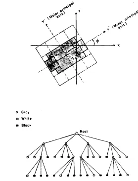
The

first

approach

[CHEE

and

AGGA-84]

is

motivated

by

the

concepts

of _{centroid and principal axes}

from

_mechanics.

These

_{are geometric}

properties of an object

that

are

invariant

to the

location

and

orientation of

the

object.

Prior to

generation of

the quadtree,

each

object

in

an

image is

normalized

to

a coordinate system with

the

object's

centroid as

the origin,

and with

the

principal axes

becoming

the

new

coordinate axes.

After the

centroid and principal angle

for

an object are

calculated,

the

object

is

rotated around

its

centroid

by

the

degree

of

the

principal angle.

(See

Figure

2.H.

)

A quadtree constructed

from

this

normalized object

is

no

longer

sensitive

to

translation,

or rotation.

It

is

also a

feature

of

this

algorithm

to

scale

the

image

to

a standard grid size

(preferably

a power of

two),

resulting in

a

representation

that

is insensitive

to

size.

This

feature is

being

noted,

although

it

was not

actually implemented in

this

application.

In order

to

restore an original object

from its

normalized

quadtree,

it is necessary for

extra

information

to

be

carried

along

as part of

the

data

structure.

Specifically,

a

linked list

of each

quadtree

comprising

the

image is

suggested. For each

quadtree,

information

is

stored

pertaining

to the

coordinates of

the

object

centroid, the

angle

of rotation of

the

object

(principal angle), and,

if

normalization

by

size

is

included,

fields representing

the

new standard

size,

and

the

amount

This

approach will not

necessarily

yield a minimal quadtree,

but

2.3.2.

Normalization

with

Respect to

Translation

Only

This

approach

[LI82,

et

al.]

results

in

a "minimal-cost" quadtree

for

an

image,

that

is

unique over

the

class of all

translations

of

the

image.

Minimal-cost

refers

to

a quadtree with

the

fewest

possible

leaves (non-terminal

nodes)

necessary

to

store

the

image.

Since the total

number of nodes

(terminal

and

non-terminal)

in

a

tree

is

proportional

to

the

number of

leaves in

the

tree,

the

algorithm

in

effect minimizes

the

total

number of quadtree nodes.

The

benefits

of such a representation are

obvious;

there

will

be fewer

nodes

to store,

and

fewer

nodes

involved

in

subsequent

tree traversal

operations.

This

technique

is

also of use

for

applications

involving

shape-matching.

A

simple,

intuitive

approach

to this

problem would

be

to translate

the

image in

all possible ways within

the array,

count

the

number of

leaves

required

for

the

quadtree at each

translation,

and

ultimately

choose

the tree

representation with

the

fewest

leaves.

This

is

expensive

(0(s**4),

where s

is

the

length

of

the

grid) and unnecessary, as will

be

explained

below.

The

algorithm assumes a

starting image

embedded

in the

northwest

quadrant of a

2**n

by

2**n

array.

A theorem

in

[LI82,

et

al.],

states

that

in

this case, the

optimal grid size will

be

either

2**(n-l),

or

2**n.

An

"enclosing

rectangle"

for

the

image is

defined

as

the

smallest

rectangle

that

encloses

the

image

and whose sides are parallel

to the

coordinate axes. The

image's enclosing

rectangle will

initially

abut

the

northwest corner of

the

grid. A variable LEAFCOJNTER

is initialized

-to

S**2,

where

S

is

the

original grid

length.

The

algorithm proceeds

by

recursively

reducing

the

image array

by

powers of

two

while

calculating

the

number of

leaves

needed

for the image

at

different

positions

in

the

array.

It

is

possible

to

narrow

the

number

of

translations

processed

to

within

2**(n-l)

-

1

pixels

in

the

eastern

direction,

and

2**(n-l)

-

1

pixels

to the

south. A representation with

the

fewest

possible

tree

nodes will always

be found

within

this

subset of

the

total

grid area.

(Proof

of

this

can

be found in

[LI82,

et al.].) For

any

image,

there

may be

more

than

one

translation

resulting in

a quadtree

representation with

the

smallest number of nodes.

It

is

therefore

necessary

to

methodically

choose one of

the

representations as

the

unique

one. If an ambiguous situation

occurs,

the

algorithmwill

tentatively

choose

the translation

whose northernmost BLACK pixel

is

a minimum Y value.

If more

than

one choice

for

a minimal

tree

is

still possible,

the

translation

with

the

smallest

X

value

is

chosen.

The

algorithm "translates"

the

image four

times:

by

0

pixels,

by

1

pixel

to the east,

by

1

pixel

to the south,

and

by

1

pixel

to the

southeast. After each

translation,

the

array is

compacted

to 1/4

of

its

former

size

by

replacing

every

2x2

pixel region with a

temporary

"supemode"

representing

the

contents of

the

four

nodes.

A

BLACK or WHITE

"supemode"

denotes four

pixels

being

all BLACK or all

WHITE;

a

GRAY

"supemode"

specifies a non-homogeneous region. In

the

case of all

four

pixels

being

all BLACK or all

WHITE,

LEAFCCUNTER

is

reduced

by

3,

meaning

that

one

leaf

is

sufficient

to

represent

this region,

rather

than

four.

The

process

is

repeated

recursively

on

the new,

compacted arrays until all

It

should

be

noted

that the

algorithm

does

not

actually

perform

the four

image translations.

A

"dummy"

row and column

indexed

by

zero and

initialized

to WHITE

is

added

to

the

array before

beginning,

in

order

to

simulate

translations

by

one pixel

by

changing

pixel coordinates only.

In

this algorithm,

it is

possible

to

detect

the

situation

where

the

smaller of

the two

grid sizes

(2**[n-l])

can accommodate

the

image (i.e.

when

the complete,

compacted

image lies

completely

within

the

northwest quadrant of

the

original grid size).

Space

requirements are on

the

order of

2

x

(2**n)

pixels, and

^

+ X

O _6rc> a White

Block

Root

Figure

2.H.

A

normalized

image

and

its

quadtree representation

[CHTE

and

AGGA-84]

Figure

2.1.

Example

of

lattice

points,

unit cell of a pattern [image:37.551.131.410.33.399.2] [image:37.551.190.332.469.571.2]

2.4.

Symmetry

Overview

[SCHA78]

The

second

half

of

this

paper

introduces

what are referred

to

as

the t^JCi-cUmensional

plane

symmetry

groups,

and relates

them to

a

hierarchical

image

representation.

Plane

symmetry

groups are well-known

in

the

fields

of mathematics and crystallography.

Perhaps

one of

the

most

fascinating

non-scientific applications of

these

groups can

be found

in

the

drawings

of

Dutch

artist

M.

C. Escher.

(Seven

Ecsher

drawings

are

found

at

the

back

of

this

paper.)

Plane

symmetry

groups are also

known

as

"wallpaper

groups",

as explained

by

Schattschneider

in [SCHA78]: "Patterns

which are

invariant

under

linear

ccmbinations of

two

linearly

independent

translations

repeat

at regular

intervals in

two

directions,

and

hence

their

groups are often

termed

"wallpaper

groups".

Seventeen

distinct

plane

symmetry

groups are

defined.

2.4.1.

Plane

Symmetry

Groups

The

following

six

definitions helpful

to the understanding

of

twcMJimensional plane

symmetry

groups

(classes)

are

taken

from [SCHA78]:

1.

A

"PERIODIC"

OR

"REPEATING" PATTERN

is

a

design

having

the

following

property:

There

exist

a)

a

finite

region and

b)

two

linearly

independent translations

such

that the

set of all

images

of

the

region when acted on

by

the

group

generated

by

these

translations produces

the

original

design.

-2.

The

TRANSLAITCN

GROUP

of a periodic pattern consists of

the

set of all

translations

that map the

pattern onto

itself.

3.

A UNIT

of

the

pattern

is

a smallest region of

the

plane

having

the

property

that the

set of

its

images

under

this

translation

group

covers

the

plane.

All

units

have the

same

area,

but

their outlines can

have infinite

_variation.

4.

Every

periodic pattern

has

naturally

associated

to

it

a

LATTICE

of

points;

choosing any

point

in

the pattern,

this

lattice is the

set of all

images

of

that

point when acted on

by

the

translation group

of

the

pattern.

5.

A UNIT CELL

is

a unit which

is

a parallelogramwhose vertices are

lattice

points.

The

vectors which

form

the

sides of a unit cell generate

the

translation group

of a pattern.

(See

Figure

2.1.)

In addition

to

translations,

a periodic pattern

may

also

be

mapped onto

itself

by

any

of

the

other plane

isometries:

rotations,

reflections,

or glide reflections.

6.

The

GENERATING

REGION

of a periodic pattern

is

the

smallest region of

the

plane whose

images

under

the

full

symmetry

group

of

the

pattern cover

the

plane.

Figure

2.M

shows

the

generating

regions

for

each plane

symmetry

group.

In

order

to

summarize

the

seventeen groups of plane

symmetry,

the

following

table

is

presented as

defined

by

those

in

the

field

of crystallography.

There

are

four basic

plane

transformations

involved

in

the

classification of such

tilings; they

are

translation,

rotation,

reflection,

and glide reflection.

Combinations

of

these

yield

the

seventeen

distinct symmetry

classes.

In

"full international

notation",

each

symmetry

class

is described

as a concatenation of

up

to

four

symbols.

Interpretation

of

full international

symbols

(left

to

right):

[SHUB

and

KDPT-74]:

1. letter p

or c

denotes

primitive or centered cell

2. integer

n

denotes highest

order of rotation

m

(mirror)

- _{reflection axis}

g

-no

reflection,

but

a glide-reflection axis

1

-no

symmetry

axis

4.

symbol

denotes

a

symmetry

axis at angle &

to x-axis,

with &

dependent

on n:

& =

180

for

_{n=l or}

2

45

for

n=4

60

for

n=3 or

6

symbols m,g,l are

interpreted

as

in 3.

NO

symbols

in

the third

and

fourth

position

indicate

that the

group

contains no reflections or glide-reflections.

Class

Int'l

Int'l

Class

Int'l Int'l

(short)

(full)

(short)

(full)

1

Pi

(pi)

2

p2

(p211)

3

pm

(plml)

4

pg

(plgl)

5

pmm

(p2mm)

6

prog

(p2mg)

7

pgg

(p2gg)

8

cm

(clml)

9

cmm

(c2mm)

10

p4

(p4)

11

p4m

(p4mm)

12

p4g

(p4gm)

13

p3

(p3)

14

p31m

(p31m)

15

p3ml

(p3ml)

16

p6

(p6)

17

p6m

(p6mm)

All

symbols,

with

the

exception of p31m and

p3ml,

can

be

referred

to

in

the

shortened

form,

with no

loss

of

identification

[SHUB

and

KOPT-74].

The

above

table

is

expressed

visually

in

Figure

2.L.

Figure

2.N

shows

the

effect of

applying the

seventeen

symmetry

groups on a single

s o .r

c

.2 u H e s

|

3

r

C .5 _. w M a -a o o .

_ u 2

o o c c g

'2

I

3

_

o

e

e

w

!8

2 2 2 2

0 mW S. m. M fi 4 e

2

o<

D

O

-

CO-a

_

e _

SI

m

t-.a

5

E

55

*. .

Figure

2.L.

Reprinted

from

[SCHA78]

[image:41.551.66.477.25.656.2]

-Figure

2.M.

Generating

regions

for

the

17

plane

symmetry

groups

[TANIS]

pi

IS

p211

II

1

pi ml

^

S

[image:42.551.66.480.107.587.2]

Figure

2.M.