International Journal of Innovative Technology and Exploring Engineering (IJITEE) ISSN: 2278-3075,Volume-8 Issue-12, October 2019
Abstract: Border Gateway Protocol (BGP) is utilized to send and receive data packets over the internet. Over the years, this protocol has suffered from some massive hits, caused by worms, such as Nimda, Slammer, Code Red etc., hardware failures, and/or prefix hijacking. This caused obstruction of services to many. However, Identification of anomalous messages traversing over BGP allows discovering of such attacks in time. In this paper, a Machine Learning approach has been applied to identify such BGP messages. Principal Component Analysis technique was applied for reducing dimensionality up to 2 components, followed by generation of Decision Tree, Random Forest, AdaBoost and GradientBoosting classifiers. On fine tuning the parameters, the random forest classifier generated an accuracy of 97.84%, the decision tree classifier followed closely with an accuracy of 97.38%. The GradientBoosting Classifier gave an accuracy of 95.41% and the AdaBoost Classifier gave an accuracy of 94.43%.
Keywords: Anomalies, Border Gateway Protocol (BGP), Decision Trees, Machine Learning (ML)
I. INTRODUCTION
Border Gateway Protocol (BGP) is an inter- autonomous system routing protocol used to transfer data packets over the internet. It determines packet routes by exchanging information about routing and reachability between Autonomous Systems (AS). An Autonomous System (AS) is a network or a collection of networks working under a shared operator having a precisely constructed routing policy. Every AS has its own internal topology and uses routing protocols of its own to find the best route for transferring data within devices that are connected over the same AS. BGP facilitates sharing data between different AS’s and is not concerned with the different routing protocols followed within the different AS’s.
Every individual AS can be recognized by a specific number which is available worldwide. There are only limited Autonomous System Numbers (ASNs). Furthermore, an AS can only share external routing information with its peers. BGP peers are designated routers of an AS that share information through the protocol. AS’s can only share information with its immediate peers, i.e., it cannot share information with an AS it is not connected to. Each AS must have at least one router that can execute BGP routing protocol and should be connected to at least one other AS which is also capable of executing BGP routing protocol. The connection
Revised Manuscript Received on October 05, 2019.
Anisha Bhatnagar, Amity School of Engineering and Technology, Amity University, Noida, India. Email: [email protected]
Namrata Majumdar, Amity School of Engineering and Technology, Amity University, Noida, India. Email: [email protected]
Shipra Shukla*, Assistant Professor, Amity School of Engineering and
Technology, Amity University, Noida, India.
Email:[email protected]
of two AS’s generates a path and a collection of paths generates a route. BGP utilizes path details to warrant inter domain routing without any loops. Existence of AS’s makes BGP a very flexible protocol as it is able to generate a route from even the most arbitrary topologies.
BGP, when used for routing internally in an AS, is known as Interior Border Gateway Protocol (IBGP). Similarly, when it is utilized to trade routing information externally amongst two AS’s, it is known as Exterior Border Gateway Protocol (EBGP).
The present rendition of BGP is form 4 (BGP4), which was distributed as RFC 4271 [1] out of 2006, in the wake of advancing through 20 drafts from reports dependent on RFC 1771[2] variant 4. RFC 4271 redressed mistakes, explained ambiguities and refreshed the detail with basic industry rehearses. The real upgrade was the support for Classless Inter-Domain Routing (CIDR) along with utilization of route aggregation in order to diminish the size of routing tables. 1994 onwards, BGP has been widely used over the internet for transmission of data packets.
Stopping of this facility will cause worldwide blockage of internet and denial of services to various users. This occurred in July of 2001 when Code Red, a worm, spread over the internet, and in September of the same year, Nimda virus attacked Microsoft’s web servers, also in 2003 when SQL Slammer hit the internet. Internet connectivity was denied to millions of people. These worms generated anomalies in the BGP system. Anomalies are discrepancies or outliers that do not follow the desired pattern. An anomaly, in BGP, is generated from an update message if even one of the given circumstances is encountered - An Autonomous System number being used is invalid, or one or more IP prefixes being used are reserved or invalid, or the originating AS does not own the IP prefix being used, or two or more Autonomous Systems have announced the same IP prefix or the suggested route has no substantial equal, or the suggested route does not agree with regular routing decisions [3].
These anomalies can be either Direct or Intended Disruptions, Direct and Unintended Disruptions, Indirect Attacks or Hardware Failures.
Direct and Intended Disruptions include all sorts of hijacking that may arise in various cases such as prefix and sub-prefix hijack. In this case, the assailant may declare a prefix or a sub prefix his own. This will cause a redirection of routes from the autonomous system to the hacker.
Direct and Unintended Disruptions are created by misconfigurations in BGP by route administrators. Imperfect arrangement of BGP devices can lead to declarations of utilized or unutilized prefixes.
BGP Anomaly Detection using Decision Tree
Based Machine Learning Classifiers
Advertising utilized prefixes can bring about hijacking as the prefixes are owned by different AS's, unused prefixes result in route leaks, this could cause an over-burden or blackhole to various victim AS's.
Indirect Attacks denote malicious activities intended towards Internet servers. Worms like Nimda, Code Red II and Slammer resulted in overloading the routing to the entire internet.
For Hardware Failure, AS's are connected to each other, either through a public peering by an outsider, for example, an Internet Exchange Point (IXP), or a private peering by a devoted link between peers. If one of these links collapse or if one of the core AS fails, it may result in nationwide or worldwide turmoil for lots of AS's [4].
It has therefore become the need of the hour to clearly differentiate between anomalous and non-anomalous data. Correct differentiation can improve convergence and increase security. Improving network convergence can increase network throughput and decrease the end-to-end delay [5]. It also allows us to maintain the Quality-of-Service. [6] details another way to maintain QoS.
Differentiation between anomalous and non-anomalous data can be done in a number of ways, the most popular of which are, Pattern Recognition, Time Series Analysis and Machine Learning. In this paper, a Decision Tree based Machine Learning approach has been proposed.
Machine Learning is that part of computer science that allows a machine to learn and predict trends by itself through analyzing historical data [7]. So far, it has been used in a variety of ways to achieve advancements in urban planning, healthcare, transportation, and industry [8]. Machine Learning is implemented by breaking the data into testing and training data sets, where the testing data set is generally just 1-10% of the actual data. Testing data is kept separate so as to evaluate the classifiers performance on an unseen data set.
The remaining sections are divided as follows - Section 2 details the previously done work in this field. Section 3 presents the process of dimensionality reduction followed as the data collected was large. The Machine Learning Classifiers used are explained in section 4, followed by the results in section 5, and the conclusion has been discussed in section 6.
II. LITERATUREREVIEW
Anomaly Detection in BGP has been done previously by Dai et al. Fisher Linear analysis and Markov Random Field technology feature selection algorithms were applied to elect attributes that could increase the distance between classes to the maximum value and decrease the distance in the class to the minimum value, and then implement grid search and cross-validation methods in order to fine tune the parameters of an SVM classifier to achieve F1-Score of 96.03% and an accuracy of 91.36% [9].
Ding et al applied minimum Redundancy Maximum Relevance (mRMR) feature selection algorithms to find best suited features utilized for classifying BGP anomalies and then applied Long Short-Term Memory (LSTM) and SVM algorithms for data classification. The SVM algorithm reached an F-score and accuracy of 69.97%, 70.79% and the LSTM algorithm reached an F-score and accuracy of 54.89% and 89.58% [10].
Nabil et al used the Fisher and minimum Redundancy Maximum Relevance (mRMR) feature selection algorithms to pick the best suited features. 3 variations of the mRMR algorithm: Mutual Information Difference (MID), Mutual Information Base (MIBASE), and Mutual Information Quotient (MIQ) were used, and the results of these algorithms were fed into Hidden Markov Models (HMMs) and Support Vector Machine (SVM) models to achieve an accuracy of 84.4% and 86.1% respectively [11].
Cosvic et al created Artificial Neural Networks with 2 hidden layers and applied cross validation to fix the number of neurons in the layers. Two features, AS_path and volume, were used to train the neural net. An accuracy of 99.3% and an F-measure of 94.5% was achieved [12].
Ćosović et al applied feature discretization and feature selection and generated Decision Tree, SVMs and Naive Bayes classifiers for anomaly detection. Threshold Selector metaclassifier was used to optimize F-score value. The best results were achieved with an SVM classifier with 88.8% F-score [13].
Li et al used the fuzzy rough sets approach for feature selection and reduction then trained decision tree and Effective Learning Machine (ELM) Algorithm to detect anomalies. By doing this, 92% accuracy with decision trees and 84.59% with ELM was achieved [14].
Judith D. Gardiner created three Hidden Markov Models to differentiate between natural, manmade and quiet network anomalies. Data from three worms, two natural events and four quiet periods had been used to train the HMMs, and reasonably good results on two worms, two power outages and one quiet period had been achieved. These models were able to differentiate between low load periods and events. Some differentiation between worms and natural events was also achieved [15].
III. DIMESIONALITYREDUCTION
To complete this project, data of BGP transmissions was collected. Individual data points represented the time difference between packet sending and receiving time for 109 hops. The data was calculated for 126101 packets. The original dimensionality of the dataset was (126101, 109). Principal Component Analysis (PCA) was applied for dimensionality reduction. PCA is generally used for pattern recognition in large datasets. PCA reduces dimensionality of a data set by finding new dimensions that can clearly separate similar and dissimilar data. They transform high dimensionality variables into smaller sets while retaining maximum information. This reduces complexity and computation time and makes the data easier to analyze and visualize.
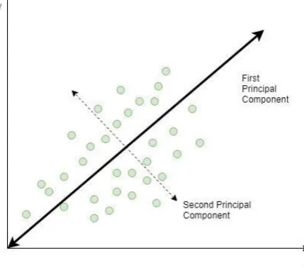
PCA generates the first principal component by finding a new dimensionality that would maximize variance as shown by Fig 1. The second principal component is generated similarly however, it is ensured that the second component is unrelated to the first. This is achieved by making the second component perpendicular to the first. PCA computes as many principal components as the original number of variables. However, it only picks those with
International Journal of Innovative Technology and Exploring Engineering (IJITEE) ISSN: 2278-3075,Volume-8 Issue-12, October 2019
Fig. 1. PCA: the thicker line shows the dimension with maximum variance
While using PCA, the value of n_components parameter is specified by the user. This value decides the number of principal components to keep. For our research, the n_components parameter was set at 2. Using PCA, the dimensionality was reduced to (126101, 2). After this, 10% of the data was kept for testing purposes and the rest was fed into the following classifiers to be trained.
IV. MACHINELEARNINGCLASSIFIERS The following classifiers were generated using the scikit-learn library available in python –
A. Decision Trees
[image:3.595.62.277.60.249.2]Decision Trees use tree like graphs or structures to represent decisions and their outcomes. It is an algorithm that only consists of conditional control statements. Each internal node signifies a test on a feature, every branch denotes an output, every ending node or leaf denotes a class name, as depicted by Fig 2. Decision Trees have less computational complexity and are able to handle both continuous and categorical data. They are also easy to interpret and generally provide high accuracy. They can be used to solve all kinds of machine learning problems like regression and classification. They can be defined on the basis of entropy and information gain, where entropy is the amount of impurity in a bunch of samples and information gain is the difference between the entropy of the parent and the child. Both these values control the split for the next node of a decision tree. A node where entropy is 0 is known as a leaf node, here all data points belong to the same class. Such a node represents a prediction. To generate this classifier min_samples_split parameter was tuned. It defines the smallest quantity of sample data points that will be needed to split an internal node. Default value is 2. A low value may often result in overfitting the classifier.
Fig. 2. A simple Decision Tree B. Random Forests
Random Forest is an ensemble machine learning technique that comprises of numerous decision trees working together. During prediction, each individual tree submits a class, the class that gets the most votes becomes the classifier’s prediction, as shown in Fig 3. Random forests generally give a higher accuracy than Decision Trees.
The reason behind this is that out of all the trees few may be wrong, many others will be right. Hence, by taking all the predictions together, the classifier is able to generate the right results. The individual trees in a random forest classifier are uncorrelated.
To generate this classifier n_estimators and max_depth parameters were tuned. n_estimators defines the count of trees working together in the forest. Default value is 10. max_depth parameter defines the maximum depth of a tree. In case no value is specified, the nodes continue to be split until all leaves are pure, i.e. they have zero impurity or all data points are of the same class, or until each leaf has data points lower than the count of min_samples_split.
C. AdaBoost
AdaBoost stands for Adaptive Boosting and can be utilized to strengthen any machine learning classifier. The default classifier it uses is a decision tree. It generates a strong classifier by joining a bunch of weak classifiers. Initially the weight for each classifier is fixed as 1/n where n represents the total count of classifiers being used. Weak classifiers are trained on the training data and added sequentially. Classes are predicted by way of computing the weighted average of the weak classifiers.
Fig. 3. Random Forest
Fig. 4. Working of an AdaBoost Classifier D. Gradient Boosting
This is an ensemble machine learning technique. It creates an ensemble of weak classifiers, generally decision trees. Gradient Boosting applies gradient descent on loss function. The aim is to minimize the loss function. To implement Gradient Boosting, first the data is fitted to a regular classifier and analyzed for errors. These errors indicate data points that are hard to fit. In the later classifiers that are sequentially added and weighted, these error points are given main focus. The resulting classifier is a combination of all classifiers with added weights. It is very flexible as it can work on a variety of different loss functions. It may be utilized in order to solve both regression and classification problems. Data pre-processing may not be required.
To generate this classifier, the value of n_estimators parameter was tuned. n_estimators defines the number of boosting predictors to execute. Other parameters include loss, criterion and min_samples_split. loss defines the loss function to be minimized. criterion defines the quality of split, i.e., it
defines the tradeoff between entropy and information gain. min_samples_split defines the minimal count of data points needed to split a node.
V. EXPERIMENTALRESULTS
A. Decision Trees
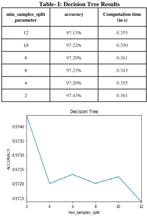
Six decision tree classifiers were generated by changing the value of the min_samples_split parameter. The value of accuracy and computation time for six values of min_samples_split: 12, 10, 8, 6, 4 and 2 was noted. Results for these have been shown in the following table, Table I.
Table- I: Decision Tree Results min_samples_split
parameter
accuracy Computation time
(in s)
12 97.13% 0.355
10 97.22% 0.350
8 97.20% 0.361
6 97.23% 0.343
4 97.20% 0.355
2 97.43% 0.361
Fig. 5. Graph showing change in accuracy with respect to change in min_samples_split
The highest accuracy achieved by a decision tree was 97.43% and was seen by using the value 2 for min_samples_split parameter. The graph given in Fig. 5, depicts the variation in accuracy with respect to the variation in the value of min_samples_split.
[image:4.595.297.537.199.554.2]International Journal of Innovative Technology and Exploring Engineering (IJITEE) ISSN: 2278-3075,Volume-8 Issue-12, October 2019
B. Random Forests
Four Random Forest classifiers were generated by changing the value of the max_depth and n_estimators parameters. The value of accuracy and computation time for 4 values of n_estimators and max_depth: 100, 50, 10, and 5 was noted. Results for these have been shown in the following table, Table II.
Table- II: Random Forests Results
n_estimators max_depth accuracy Computation
time (in s)
100 100 97.84% 15.692
50 50 97.78% 7.837
10 10 96.93% 1.397
5 5 94.21% 0.501
The highest accuracy achieved by a random forest was 97.84% and was seen by using the values 100 for n_estimators and max_depth, while the lowest computation time was noted as 0.501 seconds and was seen by using the value 5 for n_estimators and max_depth.
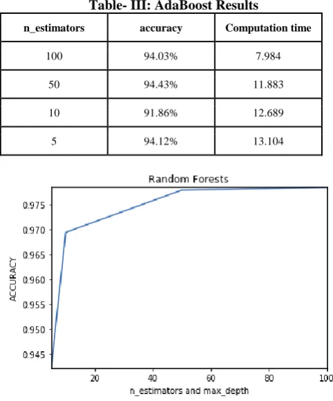
The graph given in Fig. 6, depicts the variation in the accuracy with respect to the variation in the value of the parameters. Fig. 6 for random forests shows an increase in the accuracy with an increase in the value of n_estimators and max_depth.
Value of both the parameters was taken the same for ease. An increase in the value of parameters also increased the computational time drastically. The highest computational time, as noted in table II, is 15.692 s and the lowest was noted to be 0.501 s. The highest accuracy was 97.84% and the lowest was 94.21%. Therefore, from the graph and the table, the most optimal classifier would be the one with the value of both parameters set as 100. This classifier generated an accuracy of 97.84% and computation time of 15.692 s. C. AdaBoost
Four AdaBoost classifiers were generated by changing the value of the n_estimators. The base_estimator was taken as default.
[image:5.595.310.551.53.343.2]The default base_estimator is a Decision Tree Classifier that has max_depth = 1. The value of accuracy and computation time for 4 values of n_estimators: 100, 50, 10, and 5 was noted. Results for these have been shown in the following table, Table III. The highest accuracy achieved by an AdaBoost was 94.43% and was seen by using the value 50 for n_estimators.
Table- III: AdaBoost Results
n_estimators accuracy Computation time
100 94.03% 7.984
50 94.43% 11.883
10 91.86% 12.689
5 94.12% 13.104
Fig. 6. Graph showing change in accuracy with respect to change in n_estimators and max_depth
The graph as given in Fig. 7 depicts the variation in the accuracy with respect to the variation in the value of the parameters.
Fig. 7 does not show a clear trend for change in accuracy with respect to the change in n_estimators parameter. However, from the table it can be seen that the computation time decreased with an increase in the number of n_estimators. Therefore, the most optimal classifier will be the one with the value of n_estimators set at 100. This classifier had computation time of 11.883 s and an accuracy of 94.43%.
D. GradientBoosting
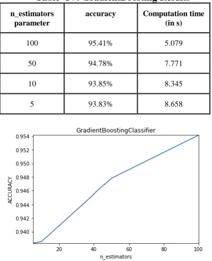
Four Gradient Boosting classifiers were generated by changing the value of the n_estimators. The value of accuracy and computation time for 4 values of n_estimators: 100, 50, 10 and 5 was noted. Results for these have been shown in the following table, Table IV.
The highest accuracy achieved by a GradientBoosting Classifier was 95.41% and was seen by using the values 100 for n_estimators. Results for these have been shown in the following table, Table IV.
From Fig. 8, it can be observed that the accuracy of a GradientBoosting Classifier increases with increase in value of n_estimators. At the same time, it can be noted from the table that the computational time decreases with an increase in the number of n_estimators.
Therefore, the most optimal classifier will be the one with the value of n_estimators set at 100. This classifier has an accuracy of 95.41% and
Fig. 7. Graph showing change in accuracy with respect to change in n_estimators
Table- IV: GradientBoosting Results n_estimators
parameter
accuracy Computation time
(in s)
100 95.41% 5.079
50 94.78% 7.771
10 93.85% 8.345
5 93.83% 8.658
Fig 8. Graph showing change in accuracy with respect to change in n_estimators
VI. CONCLUSION
Decision Tree based classification techniques are very effective in classification of anomalous BGP messages. A Random Forest classifier, on fine tuning, generates the best accuracy of 97.84% with a computation time of 15.692 seconds. A decision tree classifier, on fine tuning, generated the best accuracy of 97.38% with a computation time of 0.377 seconds. A GradientBoosting classifier, on fine tuning, generated the best accuracy of 95.41% with a computation time of 5.079 seconds. An AdaBoost classifier, on fine tuning, generated the best accuracy of 94.43% with a computation time of 11.883 seconds. Thus, Principal Component Analysis (PCA) proved to be very effective for dimensionality reduction, as it maximized variance for the newly created dimensions. This allowed the decision tree based classifiers to in turn maximize the entropy and information gain. Hence, it can be concluded that PCA followed by decision tree based classifiers such as Decision Trees, Random Forests, GradientBoosting and AdaBoost are useful for identification of anomalous BGP messages.
REFERENCES
1. https://tools.ietf.org/html/rfc4271
2. https://tools.ietf.org/html/rfc1771
3. M. Wübbeling, T. Elsner and M. Meier, "Inter-AS routing anomalies:
Improved detection and classification", In: Proc. 6th International Conference On Cyber Conflict (CyCon 2014), Tallinn, Estonia, pp. 223-238, 2014.
4. B. Al-Musawi, P. Branch and G. Armitage, "BGP Anomaly Detection
Techniques: A Survey", IEEE Communications Surveys & Tutorials, vol. 19, no. 1, pp. 377-396, 2017.
5. S. Shukla, and M. Kumar, “Improving Convergence in iBGP Route
Reflectors”, Advances in Electronics, Communication and Computing. Lecture Notes in Electrical Engineering, vol 443. Pp. 381-388, Springer, Singapore, 2018
6. S. Shukla, and M. Kumar, “An improved energy efficient quality of service routing for border gateway protocol”, Computers & Electrical Engineering, Volume 67, Pages 520-535, 2018
7. A. Bhatnagar, S. Shukla and N. Majumdar, "Machine Learning
Techniques to Reduce Error in the Internet of Things", In: Proc. of 9th International Conference on Cloud Computing, Data Science & Engineering (Confluence), Noida, India, pp. 403-408,2019.
8. N. Majumdar, S. Shukla and A. Bhatnagar, "Survey On Applications
Of Internet Of Things Using Machine Learning", In: Proc. of 9th International Conference on Cloud Computing, Data Science & Engineering (Confluence), Noida, India, 2019, pp. 562-566, 2019.
9. X. Dai, N. Wang, and W. Wang, “Application of machine learning in
BGP anomaly detection”, Journal of Physics: Conference Series, Vol. 1176, 2019
10. Q. Ding, Zhida Li, P. Batta and L. Trajković, "Detecting BGP anomalies using machine learning techniques," In: Proc. of IEEE International Conference on Systems, Man, and Cybernetics (SMC), Budapest, Hungary, pp. 003352-003355 2016.
11. N. M. Al-Rousan, and L. Trajkovic, “Machine learning models for
classification of BGP anomalies”, In Proc. of IEEE 13th International Conference on High Performance Switching and Routing, HPSR, Belgrade, Serbia, pp. 103-108, 2012.
12. M. Cosovic, O. Slobodan, and E. Junuz, “Deep Learning for Detection
of BGP Anomalies”, In: Proc. of International work-conference on Time Series (ITISE2017), Granada, Spain, pp. 95-113, 2017
13. M. Ćosović, S. Obradović and L. Trajković, "Performance evaluation
of BGP anomaly classifiers", In: Proc of Third International Conference on Digital Information, Networking, and Wireless Communications (DINWC), Moscow, Russia, pp. 115-120, 2015.
14. Y. Li, H.-J. Xing, Q. Hua, X.-Z. Wang, P. Batta, S. Haeri, and L. Trajkovic, “Classification of BGP anomalies using decision trees and fuzzy rough sets”, In: Proc. of IEEE International Conference on Systems, Man and Cybernetics, pp. 1312-1317, 2014.
J. D. Gardiner, "Multiple Markov Models for Detecting Internet
Anomalies from BGP Data," In: Proc of DoD High Performance Computing Modernization Program Users Group Conference, San Diego, CA, pp. 374-377, 2009.
AUTHORSPROFILE
Anisha Bhatnagar is currently pursuing her Bachelor’s degree in Computer science and Engineering from Amity University Uttar Pradesh. Her current research interests include Machine Learning, Deep Learning, Internet of Things and Internet routing.
Namrata Majumdar is currently pursuing B.Tech degree in Computer Science and Engineering from Amity University Uttar Pradesh. Her current research interests include Machine Learning, Iot and routing in the internet.