Visual Analysis of the Exact Solution of a Heat Equation

International Journal of Innovative Technology and Exploring Engineering (IJITEE) ISSN: 2278-3075, Volume-8 Issue-9, July 2019



Abstract: The solution of the two-dimensional heat equation is represented as images. The considered heat equation is

2 2

2 2 .

U U U

t  x y

 

  

 _  _

 _  _ , 0 x 1, 0 y 1 . The Boundary conditions are U(0, , )y t 0, (1, , )U y t 0, U x( ,0, )t 0, and

( ,1, ) 0

U x t  and the initial condition is









( , ,0) sin 4 cos 4

U x y  x  y . The images provide quick but approximate insights to the solution. Approximation by image visualization depends on many factors such as the display device, human eye factors, image resolution (sampling rate and bit depth of the image), and image resize methods. We have provided images for different time tand different resolutions We have studied the impact of different sampling rate and different image resize methods on the quality of the images. User study is performed for qualitative inspection and peak signal to noise ratio (PSNR) is used as a quantitative measure of the relative similarity in images with respect to different sampling rate and time t. Qualitative inspection and PSNR follow the same trend. Further, Qualitative inspection confirms that the quality of approximation of solution by image visualization improves with increase in sampling rate. Moreover, lanczos3 is the best interpolation method to resize the images.

Index Terms: Heat Equation, Boundary Condition, Initial Condition, Visualization, Pixel, PSNR

I. INTRODUCTION

Good visualization of the solution is an important issue, as visualization provides quick but approximate insights to the solution [1-5]. Quality of visualization of the solution depends on many factors such as the display device, human eye factors, sampling rate, interpolation technique, and bit depth of the image.

This paper presents the visual analysis of solution of two-dimensional heat equation by using the images. The considered heat equation is

2 2

2 2

U U U

t x y

 

 _{ } _ _

 

 _  _ (1)

subject to

(i) 0 x 1, 0 y 1, (ii)U(0, , )y t 0, (1, , )U y t 0,

(iii)U x( ,1, )t 0, U x y( , ,0)sin 4



 



where xand yare the space variables and t is the time variable.

Revised Manuscript Received on July 06, 2019.

Himanshu Agarwal Department of Mathematics Jaypee Institute of Information Technology, Noida, Uttar Pradesh, India

By using the separation of variable method [6] and superposition principle [6], the exact solution of the differential equation is

2

( , , ) exp(-16 ) sin(4 ) cos(4 )

U x y t   t  x  y . (2) This solution provides full information of the underlying differential equation. A mathematician can analyse the solution without any tool. However, tool is needed for a non-mathematician to analyse the solution.

The main contributions in the paper are as follows:

1. Impact of different sampling rate is discussed on the quality of the images. Three sampling rate [7] are used (grid of size 1000 1000 units, 100 100 units and 10 10 units for space variables xand y). 2. Impact of five different interpolation methods are

discussed on the quality of the images. Nearest, bilinear, bicubic, lanczos2 and lanczos3 [8] are used to resize the images.

Each image is displayed at the resolution of 1000 1000 pixels. PSNR [9] is used as quantitative quality measure of the images. Bit depth of five bits, (64 levels) [7] is used.

Key observations are as follows:

1. Visual inspection confirms that images of the grid of size 1000 1000 units, and 100 100 units are almost similar.

2. Visual inspection confirms that images of grid of size 1000 1000 units, and 10 10 units are different. 3. Lanczos3 interpolation method provides the highest

PSNR value. Therefore, Lanczos3 is the best interpolation method.

The rest of the paper is organized as follows. Proposed algorithm for image display is discussed section II. Experimental results are presented in section III. Concluding remarks are given in section IV.

II. ALGORITHM FOR IMAGE DISPLAY This section describes the algorithms for image display. The algorithms describe the display of the images of three different grid size: 1000 1000 , 100 100 , and 10 10 units. All the images are displayed at the resolution of 1000 1000 pixels.

A. Grid size of 1000 1000 units

1. x0.001: 0.001:1, y0.001: 0.001:1, t1:1:10. 2. Compute U x y t( , , )by using the equation (2). For the

fixed t, the number of grids is 1000 1000 units. 3.For the fixed t, display

the image of U x y t( , , )at the resolution of

Visual Analysis of the Exact Solution of a Heat

Equation

1000 1000 pixels. The used colormap of bit depth of five bits, (64 levels) is shown in Figure 1.

Figure 1: used colormap B. Grid size of 100 100 units

1. x0.01: 0.01:1, y0.01: 0.01:1, t1:1:10.

2. Compute U x y t( , , ) by using the equation (2). For the fixed t, the number of grids is 100 100 units 3. For fixed t, resize U x y t( , , )at 1000 1000 grid units.

Lanczos3 [8] interpolation is used to resize the ( , , )

U x y t .

4. Display the image of resized version of U x y t( , , )at the resolution of 1000 1000 pixels. The used colormap of bit depth of five bits, (64 levels) is shown in Figure 1.

C. Grid size of 10 10 units

1. x0.1: 0.1:1, y0.1: 0.1:1, t1:1:10.

2. Compute U x y t( , , ) by using the equation (2). For the fixed t, the number of grids is 10 10 units. 3. For fixed t , resize U x y t( , , )at 1000 1000 grids.

Nearest, bilinear, bicubic, lanczos2 and lanczos3 [8] interpolations are used to resize the U x y t( , , ) 4. Display the images of resized versions of U x y t( , , )at

the resolution of 1000 1000 pixels. The used colormap of bit depth of five bits, (64 levels) is shown in Figure 1.

III. EXPERIMENT AND RESULT

Experiments are done at 0.001, t1:1:10 by using the MATLAB2007b. Three different size of grids are used. The size of used grids are 1000 1000 , 100 100 and 10 10 units. PSNR is used for quantitative analysis of the images. Visual similarity between two images will be more if PSNR between two images is more or vice versa.

A. Grid size of 1000 1000 units

The images of the solution are shown in Figure 2. X axis is along left to right and Y axis is along top to bottom. In the images, blue and red circles are repeated. This represents that the solution is periodic with respect to the X and Y axes. The blue and red circles converge toward green circle with respect to time. This represents that solution decay with respect to time. These observations by using the images are similar to the results analysed by using the traditional mathematical

approach. The quantitative change in the images with respect to time is reported in the table 1. Image of Figure 2 (a) is taken as the reference image for PSNR calculations.

(a)

(b)

International Journal of Innovative Technology and Exploring Engineering (IJITEE) ISSN: 2278-3075, Volume-8 Issue-9, July 2019

(d)

(e)

(f)

(g)

(h)

(j)

Figure 2 Images of grid size of 1000 1000 units. Images are displayed at the resolution of 1000 1000 pixels. (a) t=1, (b) t=2, (c) t=3, (d) t=4, (e) t=5, (f) t=6, (g) t=7, (h) t=8,

(i) t=9, (j) t=10

Table -1 PSNR values. Reference Image is corresponding to t=1, which is shown in Figure 2 (a)

time (t) unit PSNR (dB)

2 22.7290

3 17.3672

4 14.4861

5 12.6103

6 11.2774

7 10.2815

8 9.5131

9 8.9068

10 8.4206

B. Grid size of 100 100 units

The image of the solution is shown in Figure 3.This image is corresponding to the t1. Image of Figure 2 (a) and Figure 3 represent the same solution, however at different grid size.The PSNR between the images is 27.9523 dB. Further, both images appear similar by visual inspection. This ensures that the both images represent the same solution.

Figure 3 Image of grid of size 100 100 units. The image is displayed at the resolution of 1000 1000 pixels. Lanczos3

[8] interpolation is used to resize the image. PSNR between this image and image of the figure 2 (a) is 27.9523

dB

C. Grid size of 10 10 units

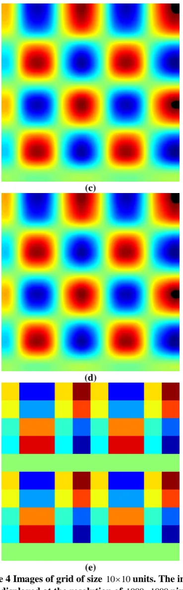
The images of the solution are shown in Figure 4. The images are corresponding to t1. Different interpolation methods, such as Nearest, bilinear, bicubic, lanczos2 and lanczos3 [8] are used. The PSNR values between the images of Figure 4 and Figure 2(a) are reported in the table 2. Important observations are as follows:

1. Images of Figure 4 appear different from the image of Figure 2 (a).

2. Method of interpolation changes the similarity of the images of Figure 4 with image of Figure 2(a). On the basis of PSNR values, methods of the interpolation are ranked as follows:

lanczos3> bilinear >lanczos2 >bicubic> nearest. Therefore, lanczos3 interpolation has the best performance and nearest interpolation method has the least performance.

(a)

International Journal of Innovative Technology and Exploring Engineering (IJITEE) ISSN: 2278-3075, Volume-8 Issue-9, July 2019

(c)

(d)

(e)

Figure 4 Images of grid of size 10 10 units. The images are displayed at the resolution of 1000 1000 pixels. Following interpolation techniques are used (a) lanczos3

(b) bilinear (c) bicubic (d) lanczos2 (e) nearest

Table -2 PSNR values of the images of Figure 4. Reference Image is shown in Figure 2 (a)

Interpolation method

PSNR (dB)

lanczos3 8.2967

bilinear 8.2196

bicubic 8.0599

lanczos2 8.1595

nearest 6.7573

IV. CONCLUSIONS

Solution of the heat equation is analysed by using the images. Images provide same insights to the solution as provided by the traditional mathematical approach. Sampling rate and interpolation methods affect the quality of the images. More sampling rate produces better image quality. Lanczos3 is the best interpolation method. Lanczos3 method provided a PSNR value of 27.95 dB for the image of grid size 100 100 units and PSNR value of 8.30 dB for the image of grid size 10 10 units.

Future scope of the work is as follows:

1. Analyse solution of more differential equation by using the images.

2. Can we solve an inverse problem? Analysis of images by using the differential equation. Efficient solution of the inverse problem can drastically improve the computation speed of image processing algorithms.

V. ACKNOWLEDGMENT

The author acknowledges research support of the Jaypee Institute of Information Technology of India.

REFERENCES

1. H. Hagen and G. Nielson Gregory and F. Post, “Report on the 2nd Dagstuhl Seminar on Scientific Visualization”, 1997.

2. C. Kelleher and T. Wagener, “Ten Guidelines for Effective Data Visualization in Scientific Publications”, Environmental Modelling & Software vol. 26 (6), pp. 822--827, 2011.

3. C. Johnson, “Top Scientific Visualization Research Problems”, IEEE Computer Graphics and Applications, vol. 24(4), pp. 13--17, 2004. 4. J. Hullman, and X. Qiao and M. Correll and A. Kale and M. Kay, “In

Pursuit of Error: A Survey of Uncertainty Visualization Evaluation”, IEEE Transactions on Visualization and Computer Graphics vol. 25 (1), pp. 903--913, 2018

5. C. Chen, “Top 10 Unsolved Information Visualization Problems”, IEEE Computer Graphics and Applications, vol. 25 (4), pp. 12--16, 2005 6. S. Salsa, “Partial Differential Equations in Action: from Modelling to

Theory”, vol. 99, 2016, Springer.

7. R. C. Gonzalez, and Woods, “Digital Image Processing”, Publishing house of electronics industry, 141 (7), 2002

8. P. Getreuer, “Linear Methods for Image Interpolation”, Image Processing On Line, vol. 1, pp. 238--259, 2011.

AUTHORS PROFILE