Abstract: In this research paper, an attempt has been made to design a Fractional order PID (FOPID) controller employed for centralized and decentralized frequency control in a restructured power system. The controller gains are optimized by Moth Flame Optimization algorithm (MFO), with Integral Time Absolute Error (ITAE) as objective function. The performance of the FOPID controller is compared with that of conventional PID controller under various contract scenarios. It is observed that FOPID as a frequency error damping controller, the steady state and dynamic performance of the proposed power system is enhanced.
Index Terms: Automatic Generation Control, Bilateral Contracts, Fractional Order Controller, Regulation.
I. INTRODUCTION
Power system control is one of the most critical and essential functions in a power market as both active and reactive power requirements are never constant and are increasing or decreasing continuously. The deviations in the frequency must be eliminated by balancing active power generation with the load through a proper control mechanism. In restructured power structure, the centralized frequency correction service is termed as Regulation or Automatic Generation Control (AGC) and the decentralized frequency regulatory service is known as Load Following (LF). Among the various control strategies, AGC [1] is the basic control structure in the power system operation. The various problems of load frequency control after deregulation have been reviewed in detail [2-6]. The major approaches used for frequency control which focus on designing proportional-integral-derivative (PID) controller [7], contemporary control approaches [8-12]. Intelligent control schemes such as neural networks [13-14] fuzzy logic-based control [15] and Soft computing-based approaches for controller parameter tuning are found in the literature. In most of the literature, PID controller has been used for eliminating the frequency error. Over the past few years, a increasing interest has been shown in fractional order controller, which has inspired many issues in the fields of
Revised Manuscript Received on August 03, 2019.
S. Jennathu Beevi, Department of EEE, B. S. AbdurRahman Crescent Institute of Science and Technology, Vandalur, Chennai, (Tamilnadu), India. E-mail: [email protected]
R. Jayashree, Department of EEE, B. S. AbdurRahman Crescent Institute of Science and Technology, Vandalur, Chennai, (Tamilnadu), India.
automation, robotics, energy systems, etc. to be solved efficiently. The authors in [16-17] have applied fractional-order proportional–integral–derivative controller (FOPID) for automatic generation control (AGC). The authors in [18] have analyzed “deregulated AGC Multi area system using FOPI and FOPID cascaded controller with geothermal, solar and thermal power plants". Rajesh [19] has applied load following controller for AGC in restructured power system. For frequency regulation in conventional power system as well as restructured power system, mostly the traditional PID controller has been used. Even though, the PID controller exhibits good dynamic performance characteristics, alternate controllers like FOPID are applied for frequency control in conventional vertically integrated utilities and restructured power structure as well. Also, PID controller has only three gains Kp, Ki and Kd as tuning parameters, whereas FOPID controller has five tuning parameters, Kp, Ki, Kd, λ and μ. The additional two degree of freedom makes the FOPID more adaptable and robust. According to the optimization theorem of No-Free-Lunch (NFL) [20], not all algorithms can solve all the issues of optimization. Fractional order systems are based on fractional order calculus [21-22] which, with few coefficients, can represent dynamic systems with high order dynamics and complicated nonlinear phenomena. The dynamics of the integer-order portray the particular and lower class of fractional-order systems.Thus, as established by many researchers, such as [23-24], fractional-order controllers surpassed their counterparts in the integer-order. The author in [25], proposed MFO, a nature inspired optimization algorithm. In recent years, MFO algorithm has been found effective for many of the power system optimization problems [27-30]. Even though there are many population-based algorithms available for optimization, MFO has been chosen in our present work because of its simplicity does not need any information about the system, (i.e.) the mathematical background of the proposed system. Being a population-based algorithm, local optima is avoided which makes it suitable for practical applications. MFO can also handle constrained and unconstrained problems.
Optimal Fractional Order PID Controller for
Centralized and Decentralized Frequency
Control in Restructured Power System
Optimal Fractional Order PID Controller for Centralized and Decentralized Frequency Control in Restructured Power System
MFO depends much on problem representation than the nature and structure of the problem. Therefore, it can be readily used for any type of optimization problem. It is observed in the literature that, MFO is highly efficient in achieving the global optimum, and is also efficient in balancing search space exploration and exploitation. Due to the adaptive convergence characteristic, MFO has very good convergence speed. Hence in our present work MFO is selected as an optimizer for minimizing the frequency error. In the literature, the performance index Integral Time Absolute Error(ITAE) is widely used for optimization. ITAE criteria gives integration of time multiplied by Absolute Error and weightage is given to those which exist over a longer time than those at the initial stage. The reduction in settling time is achieved by allocating larger multiplication factor to the error at final stages rather than the initial ones. The objectives of the present article are:(i)To Simulate the centralized and decentralized control strategy in a two-area restructured power system using PID and FOPID controller with bilateral contract structure under for different cases.(ii) To obtain the optimal controller gains using MFO algorithm by employing ITAE as objective function. And (iii) To prove the effectiveness of FOPID controller over PID via qualitative and quantitative analysis of results. To prove the effectiveness of the FOPID controller and MFO algorithm, the system given in [19] is taken for simulation.
II. SYSTEM UNDER STUDY
A. Components of the proposed system
[image:2.595.309.541.241.493.2]In the proposed system [19], there are two control areas in which each area has two GCs and two DCs respectively. Both the GCs are having non-reheat thermal units and the DCs which have the liberty of any GC to contract. Any DC in region1 may contract separately through bilateral transactions with any GC in another control region, say Area-2. The Disco Participation Matrix (DPM) shows the different Contract Participation Factors (fcp) agreements that occur between GCs and DCs.
Fig. 1 Structure of two- area interconnected power system in competitive market
The diagonal blocks of the DPM given by equation.4 corresponds to local demands i.e the demands of DCs in an area from the GCs in the same area. The demand of the DCs in one area from the GCs in another area is represented by the off-diagonal blocks.
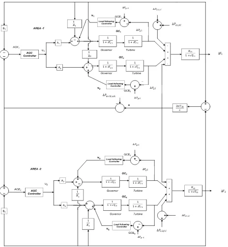
Fig.1 illustrates the competitive two area power system. The two-area interconnected system transfer function model is shown in Fig.2.The notations used in the block diagram are explained in Appendix I.As shown in Fig.2, in the two-area interconnected system, the governor, turbine and the power system are represented by their equivalent transfer function models. In each area there is an AGC controller to distribute the ACE errors to the areas.
1 1 + 𝑠𝑇𝑇2
𝐾𝑃1
1 + 𝑠𝑇𝑃1
1 1 + 𝑠𝑇𝐺2
∆𝑃𝐿1,𝑈𝐶
1 𝑅2
∆𝑃𝐿1,𝐿𝐶
1 1 + 𝑠𝑇𝐺4
1 1 + 𝑠𝑇𝑇4
𝐾𝑃2
1 + 𝑠𝑇𝑃2
- + + -
1 𝑅4
∆𝑃𝐿2,𝑈𝐶
2𝜋𝑇12
𝑠 ∆𝑃𝑔1
∆𝑃𝑔3
∆𝑃𝐿2,𝐿𝐶
∆𝑃𝑔𝑐3
∆𝑃𝑔2
∆𝐹2
∆𝑃𝑔𝑐4
- + + -
∆𝑃𝑡𝑖𝑒 12,𝑠𝑐ℎ
∆𝐹1
∆𝑃𝑔𝑐1
∆𝑃𝑔𝑐2
1 1 + 𝑠𝑇𝐺3
1 1 + 𝑠𝑇𝑇3
1 1 + 𝑠𝑇𝑇1
1 1 + 𝑠𝑇𝐺1 1
𝑅1
1 𝑅3
Fig. 2 Decentralized and Centralized frequency control scheme for two area restructured power system[19]
This functions as a primary control mechanism to bring to zero the deviations in frequency and tie line power.Each generating unit is supported by a load following controller locally which helps the generation units to supply the power contracted by the loads.The ACE signal is given as input to
the AGC controller.For the load following
controller,Generation Control Error (GCE) is given as input signal.Parameters of the framework used for simulation are given in Appendix. II.
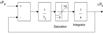
[image:2.595.61.277.567.724.2]Fig. 3 Generation Rate Constraint
Bilateral contract between a GC and a DC can be related by DC participation Matrix known as DPM. Asthe proposed system has NG =4 and ND =4, the DPM will be of the order of 4 x 4.
44 43 42 41
34 33 32 31
24 23 22 21
14 13 12 11
fcp fcp fcp fcp
fcp fcp fcp fcp
fcp fcp fcp fcp
fcp fcp fcp fcp
DPM (1)
The GCs and DCs are represented by the rows and column of the DPM matrix respectively. The fcp is the ratio of the power demanded from mth GC to the total demand of nthDC. In this matrix, the sum of all the entries in a column is unity.The contracted power of GCs with DCs is given by
NDC
n mn Ln
gcm cpf P
P
1
(2)
where ΔPgcm is the contracted power of mthgenerating unit,
ΔPLn total demand of nthDC and fcpmn contract participation
factor between nthDC and mthGC. The scheduled steady state power flow on the tie-line is given as,
∆Ptie12, sch= (Demand of DCs in area-2 from GCs in area-1) – (Demand of DCs in area-1 from GCs in area-2) (3)
The scheduled power flow on the tie-line at steady state is calculated as,
2
1 4
3
4
3 2
1 ,
12
m n m n
Ln mn Ln
mn sch
tie cpf P cpf P
P
(4)
The tie-line power error, ΔP tie12, err is the difference
between the actual power flow and the scheduled power flow. The actual tie-line power flow is equal to the scheduled power flow at steady state. Hence, tie-line power error,
ΔPtie12,err reduces to zero. The ACE signals are generated
using this error signal.
err tie i i
i B F P
ACE 12,
(5)
The contracted power of DCs are illustrated in Fig.4 In each area two types control actions take place. The first one is Frequency Regulation or AGC which is the centralized control. AGC controller is fed with ACE as input signal. The other one is Load Following (LF) action which is a decentralized control. As seen from the above figure, the
contracted load signal ΔPgcn originates from a nth DC is
compared with the generated output signal of mth GC, ΔPgm.
This is applicable while mth GC and nth DC are in contract. The difference between ΔPgcn and ΔPgm is known as
Generation Control Error (GCE). This is given as input command signal to the LF units. The LF controller reduces GCE by following the load. By minimizing this error, the generating units are made to supply the contracted power to the loads.
GCE for the load following units are given by Eqn. (6)
gm gcn
m P P
GCE
(6)
ΔPL1, LC is the sum of contracted power demanded by DC1
and DC2. Similarly, ΔPL2, LC is the sum of contracted power
demanded by DC3 and DC4. The noncontracted demands of
DCs areΔPUC1, ΔPUC2, ΔPUC3 and ΔPUC4. The distribution of
noncontracted power is resolved by the ACE Participation Factors (fcp) among various GCs in each area at steady state. It is important to note that the apfs, A1+A2 = 1.0 in Area -1
and A3+A4 = 1.0 in Area-2.
∆𝑃𝑔𝑐1
∆𝑃𝑔𝑐2
∆𝑃𝑔𝑐3
∆𝑃𝑔𝑐4
Fig. 4 Contracted power of DCs in competitive ancillary service market
B. Case Description
[image:3.595.309.542.349.623.2]Optimal Fractional Order PID Controller for Centralized and Decentralized Frequency Control in Restructured Power System
Table 1: Description of control scenarios
Case No
AGC Load following Contra
ct Violati on Area 1 Area 2 GC 1 GC 2 GC 3 GC 4 Case 1
No No No Yes No Yes No
Case 2
Yes Yes No Yes No Yes No
Case 3
Yes Yes No Yes No Yes Yes
Case 1: Only load following, No contract violation
It is assumed that no GC participates in AGC and there is no contract violation. In Area-1, GC1 is for speed regulation and GC2 is for load following. Also, in Area-2, GC3 is for speed regulation and GC4 is for load following. Since there is no AGC, no centralized controller is available. All the DCs are assumed to have a load of 0.005 puMW each. The contracts between the GCs and DCs in both the areas are described in DPM given in Eqn. (7).
40 . 0 25 . 0 90 . 0 75 . 0 0 0 0 0 60 . 0 75 . 0 10 . 0 25 . 0 0 0 0 0
DPM (7)
Also, it is assumed that there is no contract violation. It is assumed that all the four DCs possess a load demand of 0.005 puMW which is contracted to the available GCs as per the DPM given above. Hence ΔPL1=ΔPL2= ΔPL3=ΔPL4
=0.005puMW. Therefore, the contracted local load for Area-1 is 0.01pu MW and for Area-2 is 0.01pu MW. At steady state the generating unit generates power equal to the power contracted by the respective unit given by,
gcm s
gm P
P
, (8)
It is calculated for each GC using the DPM given above using equations (2) and (8) and given in Table.2. The steady state outputs of the Gencos in Area 1 & 2 are calculated using the DPM given in Eqn. (7). The tie-line power scheduled is calculated using Eqn. (4) is -0.0015 p.uMW.
Case 2: Both AGC and load following
Table 2 illustrates the distribution of contracted power from the Gencos to the respective Discos. The GC1 and GC3 are
under AGC. The DPM is same as in Case 1.The ACE participation factors for the GC1 and GC3 are 1. GC2 and GC4
are under LF. Therefore, ACE participation factors for GC 2 and GC 4 are zero. It is also assumed that there is no non contracted demand in any of the areas. The DCs have 0.005 puMW of contracted demand which is to be met by the GC2
and GC4 since these two participate in load following. The
[image:4.595.307.548.459.521.2]GCs outputs at steady state are same as Case 1.The steady state generated outputs of the four Gencos are same as in Case 1, and the values are given in Table 3. The tie-line power scheduled is calculated using Eqn. (5) is -0.0015 p.uMW, same as in Case 1 since there is no contract violation.
Table 2: Steady state output of Gencos – Case 1 and Case 2
Genco Steady State output in puMW
ΔPg1,ss (0+0+0+0) x0.005 = 0
ΔPg2,ss (0.25 +0.1+ 0.75 + 0.60) x 0.005 = 0.0085
ΔPg3,ss (0 + 0 + 0 + 0) x 0.005 = 0
ΔPg4,ss (0.75 + 0.9 + 0.25 + 0.4) x 0.005 = 0.0115
Case 3: Both AGC and load following with contract violation
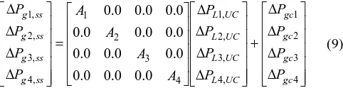
In this case, an uncontracted load demand of 0.005 puMW is introduced in Area-1.The contracted demand, DPM and APFs are same as in Case 2. This uncontracted demand along with the contracted demand of 0.005 puMW will introduce error in Area-1 ACE. This can be nullified by additional generation by the GCs in Area-1. As there are two GCs in Area-1, this uncontracted demand will be shared among the two GCs. The amount of sharing depends on the value of APFs. In the presence of uncontracted demand, the steady state power output of the GCs gets modified according to Eqn. (9). 4 3 2 1 , 4 , 3 , 2 , 1 4 3 2 1 , 4 , 3 , 2 , 1 0 . 0 0 . 0 0 . 0 0 . 0 0 . 0 0 . 0 0 . 0 0 . 0 0 . 0 0 . 0 0 . 0 0 . 0 gc gc gc gc UC L UC L UC L UC L ss g ss g ss g ss g P P P P P P P P A A A A P P P P (9)
The GC1 sharing of apf is 1 i.e, A1 = 1 and of GC2 i.e A2 =
0. Hence the additional generation will be favored by GC1 in
[image:4.595.301.553.591.834.2]Area-1.
Table 3: GENCOs output power as per Disco demands for Case 1 and Case 2
Area-1 Area-2
Total (puM
W)
DC1 DC2 DC3 DC4
Case
1 GC1 0 0 0 0 0
GC2
0.001
25 0.0005
0.003 75 0.00 3 0.008 5
GC4
0.003
75 0.0045
0.001 25
0.00 2
0.011 5 Case
2 GC1 0 0 0 0 0
GC2
0.001
25 0.0005
0.003 75
0.00 3
0.008 5
GC3 0 0 0 0 0
GC4
0.003
75 0.0045
0.001 25
0.00 2
[image:5.595.43.294.47.327.2]0.011 5
Table 4: Steady state output of Gencos – Case 3
Genco Components of
Contract violation
Steady State output in puMW
ΔPg1,ss
(A1 x ΔPL1, UC) +
ΔPgc1
(1 x 0.005) +0= 0.005
ΔPg2,ss
(A2 x ΔPL2, UC) +
ΔPgc2
(0 x 0.005) +0.0085= 0.0085
ΔPg3,ss
(A3 x ΔPL3,UC)+
ΔPgc3
(1 x 0) +0 = 0
ΔPg4,ss
(A4 x ΔPL4,UC+
ΔPgc4
(0 x 0) +0.0115 = 0.0115
The steady output of GCs in Area-1 and Area-2 during contract violation is calculated and given in Table 4. It is worthwhile to note that the power output of GC2 is 0 since A2
=0. Similarly in Area-2, A3=1 since there is no contract
violation ,the GC3 output remains same as in Case 2, Also A4
=0 which eventually result in the same power output of 0.0115 puMW.ΔPL1,UC and ΔPL2,UC are taken as 0.005 p.u
MW and the steady state output of the four Gencos are calculated using Eqn. (9), .as follows:
ΔPtie12,sch=-0.0015p.uMW. The noncontracted load
demand of 0.005 p.u MW in Area -1 is met by the generating unit under AGC i.e. GC1, while the generation of the other
Genco i.e. GC2 in area 1 at steady state is same as previous
case.
III. CONTROLLER AND OPTIMIZATION
A.FOPID controller
Fractional calculus is a generalization of the traditional integer-order calculus which encompasses fractional-order integro-differential operators. The transfer function of PIλDμ, the FOPID controller is given by
K s
s K K s
Gc( ) p i d (10)
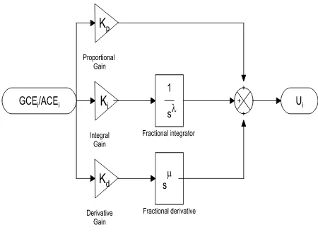
There are five parameters (Kp, Ki, Kd, and ) that have to be tuned, this improves the flexibility to meet pre-set design demands such as static errors, phase and gain margins, and robustness. The challenge of this work is to create a feasible FOPID controller that achieves the design demands by exhibiting solid efficiency. The main point is to seek acceptable differential operators’ approximations and s. The block diagram of FOPID controller is shown in Fig. 5
Fig. 5 FOPID controller
B.Objective function
ITAE is used as an objective function for FOPID controller gain tuning through optimization.
dt t P F
F ITAE
J 0t| 1|| 2|| tie|.. (11) where ΔF1 andΔF2are the system frequency deviation in
area-1 and area -2 respectively. ΔPtie is the incremental change in tie-line power and t is the time interval of simulation. The boundaries on controller gains are the constraints. The design problem can, therefore, be formulated as,
Minimize J,subjected to
PU P
PL K K
K (12a)
IU I
IL K K
K
(12b)
DU D
DL K K
K
(12c)
U
L
(12d)
U
L
(12e)
where J is the objective function denoted in (11) and the minimum and maximum bounds for the controller gains and the fractional operators are given in Eqns.12.a -12. e.
C.MFO Algorithm [25]
[image:5.595.313.538.48.212.2]Optimal Fractional Order PID Controller for Centralized and Decentralized Frequency Control in Restructured Power System
The initial population of moths is randomly generated and the evaluation criterion compares the best moths to that of the best flames, which corresponds to the best optimal values. Flames are often updated by the moths which make sure that the moths never lose best solutions and are retained as flags. The flame matrix, moth matrix, spiral motion of moth is all considered as parameters changing in each iteration. The optimization problem is assumed to be of d- dimension with n- decision variables in the search space with desired values. The search space consists a population of n-moths as search agents in which each moth has a d-dimensional vector value as the candidate solution to the issue. In d-dimensional space, the moths are flying and their positions are the potential solutions. The following n x d matrix describes the collection of moths and their positions.
nd n n d d M M M M M M M M M M 2 1 2 22 21 1 12 11 (13)
The vector OM stores the fitness values as:
n OM OM OM OM 2 1 (14)
The flames are represented by the following matrix
nd n n d d F F F F F F F F F F 2 1 2 22 21 1 12 11 (15)
The fitness values of flames are stored in a vector given as:
n OF OF OF OF 2 1 (16)
From mathematical point of view, MFO has three components:
) , ,
(I PT
MFO (17)
where I is the function which generates a random population of moths and corresponding fitness values, P is the update function and T is the termination function.
The upper and lower bound decision variables ub and lb are two vectors which are represented as follows:
] , , ,
[ub1ub2 ubd
ub (18)
] , , ,
[lb1lb2 lbd
lb
(19)
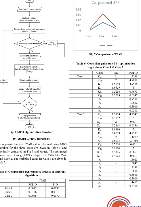
The iteration can be initiated once the function I produces the original solution and the function P runs in iterations until the termination is announced by the function T. The update feature, P is the primary component of the MFO moving moths around the search space and updating the flames position. The MFO algorithm flow chart is shown in Fig.6.
D.Implementation
For the proposed system, FOPID controller is applied for the three cases under consideration. MATLAB Simulink 2014, has been used for simulation. Moth Flame Optimization algorithm is used for optimizing the ITAE of the errors ACE and GCE of both the areas. For comparison, the PID controller is also applied for all the three cases. The parameters of the MFO algorithms are number of search agents, which is chosen as 30 and maximum number of iterations is chosen as 100. After several simulations, the
limits on the controller gains are selected
Fig. 6 MFO Optimization flowchart IV. SIMULATION RESULTS
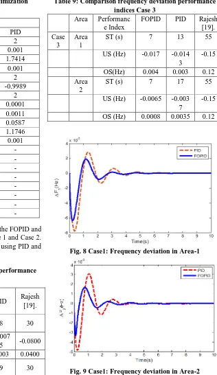
[image:7.595.50.279.50.517.2]The objective function, ITAE values obtained using MFO algorithm for the three cases are given in Table 5 and graphically compared in Fig.7 and values. The optimized gains achieved through MFO are depicted in Table 6 for Case 1 and Case 2. The optimized gains for Case 3 are given in Table 7.
Table 5: Comparative performance indexes of different algorithms
ITAE
FOPID PID
Case1 0.0012 0.0030
Case 2 0.0156 0.0318
Case 3 0.0046 0.0077
Fig.7 Comparison of ITAE
Table 6: Controller gains tuned by optimization algorithms- Case 1 & Case 2
Gains PID FOPID
Case 1 Kp1 2 1.9588
Kp2 2 4.9878
Ki1 1.9040 4.9968
Ki2 1.6529 5
Kd1 0.3250 0.7693
Kd2 0.2699 0.6142
λ1 - 0.9988
λ2 - 1.0002
μ1 - 0.5000
μ2 - 0.6515
Case 2 Kp1 1.9994 4.9945
Kp2 0.3092 5
Kp11 2 0.001
Kp22 0.2161 0.0136
Ki1 1.9996 5
Ki2 0.0099 4.9973
Ki11 2 -0.8817
Ki22 0.0011 -0.7960
Kd1 0.7010 0.001
Kd2 0.8000 5
Kd11 0.5325 0.0061
Kd22 0.4023 0.001
λ1 - 1.4025
λ2 - 1.0043
λ3 - 1.1390
λ4 - 1.5000
μ1 - 0.5000
μ2 - 0.5000
μ3 - 1.4467
[image:7.595.59.549.61.783.2]Optimal Fractional Order PID Controller for Centralized and Decentralized Frequency Control in Restructured Power System
Table 7: Controller gains tuned by optimization algorithms- Case 3
Case 3
Gains FOPID PID
Kp1 5 2
Kp2 0.001 0.001
Ki1 4.9934 1.7414
Ki2 0.3551 0.001
Kd1 5 2
Kd2 -0.7828 -0.9989
Kp11 5 2
Kp22 -0.2118 0.0001
Ki11 0.0950 0.0011
Ki22 0.001 0.0587
Kd11 1.5277 1.1746
Kd22 0.001 0.001
λ1 1.0088 -
λ2 1.0047 -
λ3 1.0003 -
λ4 0.6352 -
μ1 1.4937 -
μ2 1.0654 -
μ3 0.5058 -
μ4 1.4629 -
The quantitative performance comparison of the FOPID and PID controllers are shown in table 8 for Case 1 and Case 2. The performance indices obtained for Case 3 using PID and FOPID are compared and shown in Table 9.
Table 8: Comparison frequency deviation performance
indexes
Area
Performanc e Index
FOPID PID Rajesh
[19].
Case 1
Area
1 ST (s) 7.5 8 30
US (Hz) -0.006
4
-0.007
5 -0.0800
OS (Hz) 0.0018 0.003 0.0400
Area
2 ST (s) 7.8 9 30
US (Hz) -0.003
3
-0.004
8 -0.0800
OS (Hz) 0.0016 0.0031 0.0400
0 Case
2
Area
1 ST (s) 7 10 45
US (Hz) -0.005
8 -0.008 -0.08
OS (Hz) 0.0023 0.005 0.06
Area
2 ST (s) 10 15 45
US (Hz) -0.003 -0.005 -0.08
OS (Hz) 0.0028 0.006 0.06
Table 9: Comparison frequency deviation performance indices Case 3
Area Performanc
e Index
FOPID PID Rajesh
[19]. Case
3
Area 1
ST (s) 7 13 55
US (Hz) -0.017 -0.014
3
-0.15
OS(Hz) 0.004 0.003 0.12
Area 2
ST (s) 7 17 55
US (Hz) -0.0065 -0.003
7
-0.15
[image:8.595.230.546.67.613.2]OS (Hz) 0.0008 0.0035 0.12
Fig. 8 Case1: Frequency deviation in Area-1
[image:8.595.40.298.482.787.2] [image:8.595.41.297.483.790.2]0 1 2 3 4 5 6 7 8 9 10 -4
-2 0 2 4 6 8 10 12 14 16x 10
-4
Time(s)
P
tie
1
2
(p
u
M
W
)
PID FOPID
Fig.10 Case1: Tie-line power deviation between Area-1 and Area-2
0 1 2 3 4 5 6 7 8 9 10
-2 0 2 4 6 8 10 12 14x 10
-3
Time(s)
P gs
(p
u
M
W
)
GC1= 0 puMW GC2 = 0.0085 puMW GC3 = 0 puMW GC4 = 0.0115 puMW
Fig.11 Case1: Power outputs of GCS at steady state
Fig.12 Case2: Frequency deviation in Area-1
Fig.13: Case2: Frequency deviation in Area-2
Fig.14 Case 2: Tie-line power deviation between Area-1 and Area-2
Fig.15 Case2: Power outputs of GCS at steady state
The output responses obtained using FOPID and PID controllers for Case 1 are shown from Fig.8 to Fig.11. The output responses obtained using FOPID and PID controllers for Case 2are shown from Fig.12 to Fig.15
0 5 10 15
-20 -15 -10 -5 0
5x 10
-3
Time(s)
F
1
(H
z)
PID FOPID
Optimal Fractional Order PID Controller for Centralized and Decentralized Frequency Control in Restructured Power System
0 5 10 15
-8 -6 -4 -2 0 2 4x 10
-3
Time(s)
F
2
(H
z)
PID FOPID
Fig.17 Case 3: Frequency deviation in Area-2
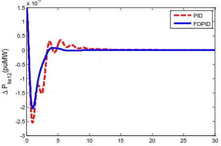
[image:10.595.67.272.63.219.2]Area-1 and Area-2 frequency deviations obtained using the optimized PID and FOPID gains for Case 3 are shown in Fig.16 and Fig.17. The tie-line power deviation and the Genco outputs are shown in Fig.18 and Fig.19 respectively. The Genco outputs for Case 3 are calculated and given in Table 10.
0 5 10 15 20 25 30
-3 -2.5 -2 -1.5 -1 -0.5 0 0.5 1 1.5x 10
-3
Time(s)
P
ti
e
1
2
(p
u
M
W
)
[image:10.595.294.555.72.268.2]PID FOPID
Fig. 18 Case 3 Tie-line power deviation between Area-1 and Area-2
Fig. 19 Case3: Power outputs of GCS at steady state
Table 10:GENCOs output power -Case 3
Area-1 Area-2
Total (puM
W) DC1 DC2 DC3
DC
4
Noncontra cted demand
GC
1
0 0 0 0 0.005 0.005
GC
2
0.00 125
0.000 5
0.003 75
0.0
03 -
0.008 5 GC
3
0 0 0 0 - 0
GC
4
0.00 375
0.004 5
0.001 25
0.0
02 -
0.011 5
V. CONCLUSION
In this work, an effort has been made to analyze the practicability of affording optimized frequency control as an ancillary service using FOPID controller optimized by MFO algorithm in a competitive power market. The performance of FOPID controller has been compared with that of the classical PID controller in the two area inter connected non-reheat thermal power system. Three different cases under bilateral contract scenario have been analyzed. The gains of the AGC and Load following FOPID controllers are optimized by the MFO algorithm using ITAE of ACE and GCE as objective function and it has been found that FOPID is effective in bringing the frequency deviation and tie line power deviations to zero. In all the three cases, the contracted amount of power demanded by the DCs has been supplied by the corresponding GCs. On comparison of the results with that of [19], the effectiveness of FOPID controller is established.
REFERENCES
1. P. Kundur, J. Paserba, V. Ajjarapu, G. Andersson, A. Bose, C. Canizares, and T. Van Cutsem, “Definition and classification of power system stability,” IEEE transactions on Power Systems, vol. 19, no. 2, 2004, pp. 1387-1401.
2. R. Christie, D. and A. Bose, “Load frequency control issues in power system operations after deregulation,” IEEE Transactions on Power systems, vol. 11, no. 3, 1996, pp. 1191-1200.
3. E. Hirst, and B. Kirby, “Separating and measuring the regulation and load-following ancillary services,” Utilities Policy, vol. 8, no. 2, 1999, 75-81.
4. V. Donde, M. A. Pai, and I. A. Hiskens, “Simulation and optimization in an AGC system after deregulation,” IEEE transactions on power systems, vol. 16, no. 3, 2001, pp. 481-489.
5. E. Nobile, A. Bose, and K. Tomsovic, “Feasibility of a bilateral market for load following,” IEEE Transactions on Power systems, vol. 16, no. 4, 2001, pp. 782-787.
[image:10.595.52.278.340.489.2] [image:10.595.51.285.357.700.2]7. P. Bhatt, R. Roy, and S. P. Ghoshal, “Optimized multi area AGC simulation in restructured power systems,” International journal of electrical power & energy systems, vol. 32, no. 4, 2010, pp. 311-322. 8. F. Liu, Y. H. Song, J. Ma, S. Mei, and Q. Lu, “Optimal load-frequency
control in restructured power systems,” IEE Proceedings-Generation, Transmission and Distribution, vol. 150, no. 1, 2003, pp. 87-95. 9. I. A. Chidambaram, and B. Paramasivam, “Optimized load-frequency
simulation in restructured power system with redox flow batteries and interline power flow controller,” International Journal of Electrical Power & Energy Systems, vol. 50, 2013, pp. 9-24.
10.P. Dahiya, V. Sharma, and R. Naresh, “Automatic generation control using disrupted oppositional based gravitational search algorithm optimised sliding mode controller under deregulated environment,” IET Generation, Transmission & Distribution, vol. 10, no. 16, 2016, pp. 3995-4005. 11.G. Sharma, K. R. Niazi, and R. C. Bansal, “Adaptive fuzzy critic based
control design for AGC of power system connected via AC/DC tie-lines,” IET Generation, Transmission & Distribution, vol. 11, no. 2, 2017, pp. 560-569.
12.S. H. Hosseini, and A. H. Etemadi, “Adaptive neuro-fuzzy inference system based automatic generation control,” Electric Power Systems Research, vol. 78, no. 7, 2008, pp.1230-1239.
https://doi.org/10.1016/j.epsr.2007.10.007
13.H. Shayeghi, H. A. Shayanfar, and O. P. Malik, “Robust decentralized neural networks based LFC in a deregulated power system,” Electric Power Systems Research, vol. 77, no. 3-4, 2007, pp. 241-251.
14.L.C Saikia, S. Mishra, N. Sinha, and J. Nanda, “Automatic generation control of a multi area hydrothermal system using reinforced learning neural network controller,” International Journal of Electrical Power & Energy Systems, vol. 33, no. 4, 2011, pp. 1101-1108.
15.H. Shayeghi, H. A. Shayanfar, and A. Jalili, “Multi-stage fuzzy PID power system automatic generation controller in deregulated environments,” Energy Conversion and management, vol. 47, no. 18-19, 2006, pp. 2829-2845.
16.T. S. Gorripotu, H. Samalla, C. J. M. Rao, A. T. Azar, and D. Pelusi, “TLBO Algorithm Optimized Fractional-Order PID Controller for AGC of Interconnected Power System,” In Soft Computing in Data Analytics,
2019, (pp. 847-855). Springer, Singapore.
17.Y. Arya, “AGC of restructured multi-area multi-source hydrothermal power systems incorporating energy storage units via optimal fractional-order fuzzy PID controller,” Neural Computing and Applications, vol. 31, no. 3, 2019, pp. 851-872.
18.Z. X. Tang, Y. S. Lim, S. Morris, J. L. Yi, P. F. Lyons, and P. C. Taylor, “A comprehensive work package for energy storage systems as a means of frequency regulation with increased penetration of photovoltaic systems,” International Journal of Electrical Power & Energy Systems, vol. 110, 2019, pp. 197-207.
19.R. J. Abraham, D. Das, and A. Patra, “Load following in a bilateral market with local controllers,” International Journal of Electrical Power & Energy Systems, vol. 33, no. 10, 2011, pp. 1648-1657.
20.D. H. Wolpert, and W. G. Macready, “No free lunch theorems for optimization,” IEEE transactions on evolutionary computation, vol. 1, no. 1, 1997, pp. 67-82.
21.K. B. Oldham, and J. Spanier, “The fractional calculus theory and applications of differentiation and integration to arbitrary order,”
Academic Press, New York, 1974, PP. 111.
22.K. S. Miller, and B. Ross, “An Introduction to the Fractional Calculus and Fractional Differential Equation,” Wiley, New York, 1993.
23.I. Podlubny, “Fractional-order systems and PI/sup/spl lambda//D/sup/spl mu//-controllers,” IEEE Transactions on automatic control, vol. 44, no. 1, 1999, pp. 208-214.
24.R. El-Khazali, W. Ahmad, and Y. Al-Assaf, “Sliding mode control of generalized fractional chaotic systems,” International Journal of Bifurcation and Chaos, vol. 16, no. 10, 2006, pp. 3113-3125.
25.S.Mirjalili, “Moth-flame optimization algorithm: A novel nature-inspired heuristic paradigm,” Knowledge-Based Systems, vol. 89, 2015, pp. 228-249.
26.S. Reddy, L. K. Panwar, B. K. Panigrahi, and R. Kumar, “Solution to unit commitment in power system operation planning using binary coded modified moth flame optimization algorithm (BMMFOA): a flame selection based computational technique,” Journal of Computational Science, vol. 25, 2018, pp. 298-317.
27.B. V. S. Acharyulu, B. Mohanty, and P. K. Hota, “Comparative performance analysis of PID controller with filter for automatic generation control with moth-flame optimization algorithm,” In Applications of Artificial Intelligence Techniques in Engineering, 2019, (pp. 509-518). Springer, Singapore. https://doi.org/10.1007/978-981-13-1819-1_48
28.A. K. Barisal, AND l. K. Lal, “Application of moth flame optimization algorithm for AGC of multi-area interconnected power systems,” International Journal of Energy Optimization and
Engineering (IJEOE), vol.7, no. 1, 2018, pp. 22-49.
29. M. A. Taher, S. Kamel, F. Jurado, and M. Ebeed, “An improved moth‐flame optimization algorithm for solving optimal power flow problem,” InternationalTransactions on Electrical Energy Systems, vol. 29, no. 3, 2019, pp. e2743.
Appendix I Nomenclature
GC Genco
DC Disco
∆PL Change in Load Demand
Kp Gain of the power system
Tp Time constant of the system (s)
Tt Time constant of the turbine (s)
Tg Time constant of the Governor (s)
T12 Time constant of the tie-line (s)
R Speed regulation (Hz/p.u.MW)
∆F Frequency deviation (Hz)
∆Ptie12 Deviation in Tie line power exchange
between Area -1 and Area-2
∆PL1,UC Un-contracted load demand
A1,A2 ACE participation factors of GCs 1 & 2 in
area-1
A3,A4 ACE participation factors of GCs 3 &4 in
area-2
B1, B2 Frequency bias factors
Kp1,Ki1,Kd1λ1,µ
1
Gains of Load following controller for GC2
Kp2,Ki2,Kd2λ2,µ
2
Gains of Load following controller for GC4
Kp11,Ki11,
Kd11λ3,µ3
Gains of AGC controller in area-1
Kp22,Ki22, Kd22
,λ4,µ4
Gains of AGC controller in area-2
Appendix IINominal Values Of System Parameters
Kpi= 120
Tgi=0.08 s
Tti=0.3 s
Tpi = 20 s
Ri=2.4 Hz/pu.MW
Bi= 0.425
Tij = 0.0866
AUTHORSPROFILE
Optimal Fractional Order PID Controller for Centralized and Decentralized Frequency Control in Restructured Power System