Simulation-Based Inference on Mixture Experiments

Rochester Institute of Technology

RIT Scholar Works

Theses

4-19-2019

Simulation-Based Inference on Mixture

Experiments

Tejasv Bedi

Follow this and additional works at:

https://scholarworks.rit.edu/theses

This Thesis is brought to you for free and open access by RIT Scholar Works. It has been accepted for inclusion in Theses by an authorized administrator of RIT Scholar Works. For more information, please [email protected].

Recommended Citation

M

T

Simulation-Based Inference on Mixture

Experiments

Author:

Tejasv BEDI

Supervisor:

Dr. Robert PARODY

A thesis submitted in partial fulfillment of the requirements for the degree of Masters of Science

in

Applied Statistics College of Science

Department of Mathematical Sciences

ROCHESTER INSTITUTE OF TECHNOLOGY

Abstract

School of Mathematical Sciences

Masters of Science

Simulation-Based Inference on Mixture Experiments

by Tejasv BEDI

Acknowledgements

Contents

Abstract v

Acknowledgements vii

1 Introduction 1

1.1 Mixture Experiments . . . 1

1.2 Simulation Experiments . . . 2

1.3 Study Layout . . . 2

2 Background 3 2.1 Introduction to Mixture Experiments and Models . . . 3

2.1.1 Simplex-Lattice Design . . . 3

2.1.2 Simplex-Lattice Model Equations. . . 4

2.2 Parameter Estimation for a{q, 2}Simplex-Lattice Design . . . 6

2.3 Moments of Parameter Estimates . . . 8

2.3.1 Expectation of Parameter Estimates . . . 9

2.3.2 Variance of Parameter Estimates . . . 10

2.3.3 Covariance of Parameter Estimates. . . 10

2.4 Estimate of Predicted ResponseYb(x) . . . 11

2.5 Pseudocomponents . . . 11

2.6 Cholesky’s Decomposition . . . 14

3 Literature Review 17 3.1 Simulation-Based Multiple Comparisons . . . 17

3.1.1 Efficiency Study of a One-Way Layout . . . 18

3.1.2 Efficiency Study of an Analysis of Covariance Layout . . . 19

3.2 Simulation-Based Methods for Response Surface Designs . . . 19

3.3 Confident Visualization Techniques in the analysis of Mixture Exper-iments . . . 21

4 Research Method 25 4.1 Theory behind the Simulation-Based Method . . . 25

4.2 Use of L-pseudocomponents. . . 28

5 Data Examples 31 5.1 Artificial Sweetener Experiment. . . 31

5.2 Tropical Beverage Experiment . . . 33

6 Discussion and Conclusions 35

List of Figures

2.1 Experimental regions of a{3,m}Simplex-Lattice Designs . . . 4

2.2 The simplex region based on the constraints x1 0.2, x2 0.2 and x3 0.4 . . . 12 2.3 Experimental regions for the upper bound examples, (A)

experimen-tal region for example 1; (B) experimenexperimen-tal region for example 2. . . 13

2.4 Experimental region for the example with both lower and upper bounds, restricted by 0.15 x1 0.3, 0x20.25 and 0.5 x30.85 . . . . 14 4.1 Pseudocomponents and Point coverage in the Simplex Region (l and

f are indices approximating the number of points and pseudocompo-nents respectively ) . . . 29

5.1 Artificial Sweetner Example; (a) Estimated Improvement contours rel-ative to the centroid; (b) simulation-based lower 95% simultaneous confidence bounds. The region inside the zero contour indicates im-provement over the control settings . . . 32

List of Tables

2.1 Upper Bound examples . . . 13

5.1 Data from the Artificial Sweetener Experiment . . . 31

5.2 Data from the Tropical Beverage Experiment . . . 33

6.1 Approximate sample-size savings, two-sided simulation-based method to the Sa and Edwards (1993) adaptation of the Scheffé method at

Chapter 1

Introduction

1.1 Mixture Experiments

Over the years, experimentation in fields such as analytical chemistry, industrial en-gineering and, applied mathematics and statistics has revolved around optimizing some operational factors or components to obtain desirable properties in the final product, under some given experimental conditions. Response Surface Experiments provide a foundation to extract meaningful relationships between several explana-tory variables and one or more response variables. Once such an experiment is de-signed, it allows a practitioner to discover the desirable settings of the explanatory variables that optimize a given set of response variables. To mathematically model this experiment, Box and Wilson suggested a second-degree polynomial model as an approximation to such experiments.

Mixture Experiments are a special case of response surface experiments that allows an experimenter to optimize the proportions of ingredients for a fixed quantity of those ingredients. The response variable in these experiments only depend on the proportions of the ingredients and not their total amount being used. These experi-ments are modeled as polynomials with the given restriction that all the component proportions must add up to one. Given the nature of the model and the restriction applied to it, suppose we are includingqexperimental components to formulate a product, then the experimental region withq = 3 components can be plotted as a triangle, forq=4 we will obtain a tetrahedron, and so on.

Let us consider an example of a Mixed fruit juice and the ingredients used to cre-ate one. Suppose we combine three fruits namely apple, lemon and orange to crecre-ate a Mixed Fruit drink. It would be of the greatest interest to the manufacturer to dis-cover the perfect blend that creates a flavor, well received by the consumers. The flavor of a drink is highly sensitive to the proportion of components it comprises of. Therefore, different manufacturers advertise similar fruit drinks that are quite differ-ent in taste because of a differdiffer-ent composition of ingredidiffer-ents. Mixture Experimdiffer-ents help manufactures in optimizing desired response variables based on the mixture of component blends of substances which is generally hard to capture . Getting back to the example, suppose, the manufacturer wants to market the Mixed Fruit drink as having a highly tangy flavor. By running a mixture experiment, he will be able to discover if any particular ingredient is the root cause of tanginess in the drink, or if any blend of certain ingredients is the reason for that flavor which the manu-facturer is looking for. There is a huge possibility that lemon or orange alone might not contribute much towards the desirable flavor, but it could be possible that a bi-nary blend of both the ingredients in equal proportions(50% : 50%)are extracting

2 Chapter 1. Introduction

ingredients that optimize the final product, mixture experiments become a neces-sity. The manufacturer would have missed on such an important result without the application of such experiments.

1.2 Simulation Experiments

In recent times, technology is improving at an exponential rate, trying to meet the requirements of the industry and the working sector. There has been a lot of fo-cus on increasing processing power and speed to enable multitasking and carrying out computationally heavy operations that were once only possible in theory. One such domain was that of Simulation Experiments. Traditionally, research in such a field was only restricted to theoretical aspects of statistics. Having to apply these techniques on data sets and extracting meaningful results involved a lot of time and cost. This was one of the biggest drawback of these methods. At present, all com-puters are being incorporated with an amazing processing power, that too at a mod-est price. This is because it has become an absolute necessity for running modern day applications, and carrying out multitasking and efficient programming. For in-stance, a social networking site could be using complex algorithms, neural networks and artificial intelligence in ways that one could never imagine. Hence, Simulation Methods that were previously not considered feasible, demonstrate a lot of research potential and modern day applications to statistical problems. Monte Carlo Simula-tion methods help in solving complex problems using random sampling, optimiza-tion, numerical procedures and probability distributions. Simulation is generally applied in situations when a closed form solution is unobtainable using the usual mathematical tools. We would be using this technique for our research method to encounter the same problem.

1.3 Study Layout

Chapter 2

Background

2.1 Introduction to Mixture Experiments and Models

The concept of mixture experiments came into existence when there was a need to mathematically formalize experiments that involved mixing various ingredients or components, to gain insight on the properties of each blend individually, as well as their various combinations with each other. To approach these designs from a mod-eling perspective, we associate them with polynomial models that were introduced by Scheffé in the early years (1958-1965). This approach has been believed to be the foundation of mixture experiments, as claimed by many renowned scientists and re-search scholars. The most essential property of these models that differentiate them from other polynomial models is the addition of a specific restriction on the input space. The restriction being that, all the proportions of component blends must add up to unity, i.e. x1+x2+. . .+xq = 1. Using this constraint, we are able to

mod-ify the polynomial model equations, and observe some interesting properties of the mixture model. We would now proceed with discussing a basic type of a mixture design.

2.1.1 Simplex-Lattice Design

A simplex-lattice design is used when a polynomial equation is used to represent a response surface over an entire simplex region. The points plotted on the region are equally spaced and have the restriction of all the components adding up to 1. A

{q,m}simplex-lattice design can be expressed as a design with qcomponents and

m+1 equally spaced points such that the component proportions are

xi =0,_m1,_m2, . . . , 1

where mcan be defined as the highest degree of blending included in the design space. For eg. for binary blending we have m = 2, for ternary blending we have

m = 3 and so on. To visualize a {q,m} simplex-lattice design, we illustrate two examples in Figure 2.1. In this figure, the design points for pure blends(x1,x2,x3) are given by(1, 0, 0), (0, 1, 0)and (0, 0, 1) such that 1 denotes the presence of that

particular component in the order of (x1,x2,x3) and 0 denotes the absence of the components in that particular blend. For pure blends, only one component is con-sidered at a time. Considering binary blends, two components are blended together in equal proportions at a time. Hence, the components(x1,x2,x3)will take values

4 Chapter 2. Background

(1/3, 1/3, 1/3). The centroid represents the ternary blending of the all the 3 compo-nents in equal proportions.

(A) {3,2} Simplex-Lattice Design (B) {3,3} Simplex-Lattice Design

FIGURE 2.1: Experimental regions of a {3,m} Simplex-Lattice De-signs

2.1.2 Simplex-Lattice Model Equations

The general equation of anmth_{degree polynomial regression model is given by}

Y(x) =b0+

q

Â

i=1

bixi+ q

Â

Â

ij

bijxixj+ q

Â

Â

Â

ijk

bijkxixjxk+. . . (2.1)

Y(x)is the response, given a vector of known values x; bs are the population

pa-rameters or the model coefficients that are fixed but unknown andxi,xj,xk, . . . are

explanatory variables that are known to us.

The key here is to derive the equation for a{q,m}simplex-lattice design by multi-plying some of the terms of equation (2.1) by the restriction (x1+x2+. . .+xq) =1.

The resulting equation would be addressed as the "canonical" form of the polyno-mial equation. To demonstrate the proof, we will consider linear and quadratic re-gression models and use the restrictions to derive model equations for_{q, 1_} and

{q, 2}simplex-lattice designs respectively.

Considering a linear regression model

Y(x) =b0+

q

Â

i=1

bixi (2.2)

The model restriction is given by

q

Â

i=1

Substituting (2.3) in (2.2) we have

Y(x) = b0

q

Â

i=1

xi

! +

q

Â

i=1

bixi (2.4)

=

q

Â

i=1

(b0+bi)xi

Y(x) =

q

Â

i=1

b⇤_ixi (2.5)

Whereb⇤_i = b0+bifor alli=1, 2, . . .q

Now we work on a quadratic regression equation to derive a{q, 2}simplex-lattice, in a similar fashion.

The second degree polynomial equation is given by

Y(x) =b0+

q

Â

i=1

bixi+ q

Â

i=1

biix2i + q

Â

Â

i<j

bijxixj (2.6)

Now, modifying equation (2.3) we have

xi+ q

Â

j6=i

xj =1

xi =1 q

Â

j6=i

xj (2.7)

x_i2= xi 1 q

Â

j6=i

xj

!

(2.8)

Substituting equations (2.3), (2.7) and (2.8) in (2.6), we get

Y(x) =b0

q

Â

i=1

xi

! +

q

Â

i=1

bixi+ q

Â

i=1

biixi 1 q

Â

j6=i

xj

! +

q

Â

Â

i<j

bijxixj

=

q

Â

i=1

(b0+bi+bii)xi q

Â

i=1

biixi q

Â

j6=i

xj

! +

q

Â

Â

i<j

bijxixj

Y(x) =

q

Â

i=1

b⇤_ixi+ q

Â

Â

i<j

b⇤_ijxixj (2.9)

Using a similar derivation technique we can also obtain the equation of{q, 3}cubic model given by

Y(x) =

q

Â

i=1

b⇤_ixi+ q

Â

Â

i<j

b⇤_ijxixj+ q

Â

Â

i<j

dijxixj(xi xj) + q

Â

Â

Â

i<j<k

b⇤_ijkxixjxk (2.10)

Y(x) =

q

Â

i=1

b⇤_ixi+ q

Â

Â

i<j

b⇤_ijxixj+ q

Â

Â

Â

i<j<k

6 Chapter 2. Background

where, (2.11) is a special case of a cubic model in which the termdijxixj(xi xj)is

not considered.

From this point onward, we will remove the asterisks (*) frombcoefficients, as they

were just used to differentiate the simplex model equations from general polynomial equations.

Now we explain the significance of the coefficients of the simplex-lattice model equa-tions. We first consider the simple case of{q, 1} and{q, 2}models. Suppose, we have pure components without the presence of blending. Then, in equations (2.5) or (2.9), if we consider a componenti, we will substitutexi = 1, this would result in

xj = 0 for all j6= i. Hence, we obtainY(x) = bi. Therefore,bi can be defined as the

expected change or response to the pure componenti. Moving on to a situation of linear blending. Suppose there exists a linear blending between componentsiand

j, then the model equation is represented byY(x) = bixi+bjxj (using (2.5)), where

xi and xj add up to 1 and xk = 0 for all k 6= i,j. There could be a situation that

by using equation (2.5), the model is under fitting the data, which could result in a loss of information. The reason of this situation might be the unaccounted presence of two-way interactions or binary blending. Then, by fitting equation (2.9) instead, we will obtainY(x) = bixi+bjxj+bijxixj. The termbijxixj could be computed by

taking the difference between equations (2.9) and (2.5). If the excess, represented by the term bijxixj is positive, orbij > 0, then the excess is considered as the

syner-gism of the binary mixture, wherebijis the second-order model coefficient of binary

synergism. On the contrary, if bij < 0, the deficit is called the antagonism of the

binary mixture. Similarly, if a cubic model is better suited for the situation, then in equation (2.10), the termdijxixj(xi xj)represents an excess or synergism. While,

dij is the cubic coefficient of the binary synergism between xi andxj. If dij 6= 0, the

termdijxixj(xi xj)could take negative as well as positive values resulting in

syn-ergistic and antagonistic blending between the two components. The termbijkxixjxk

represents ternary blending in the model, wherebijkis the third order coefficient of

ternary synergism.

In the next section, we will discuss about the parameter estimation of simplex-lattice design models.

2.2 Parameter Estimation for a

{

q

, 2

}

Simplex-Lattice Design

The parameters in the{q,m}polynomials are expressible as simple functions of the expected responses at the points of the_{q,m_}simplex-lattice designs. In this section, we will discuss the parameter estimation for a{q, 2}Simplex-Lattice Design that in-volves a quadratic model equation.

The model equation for a quadratic model can be written as

yu= q

Â

i

bixi+ q

Â

Â

i<j

bijxixj+#u (2.12)

Let the equation of predicted response be given as

b yu=

q

Â

i=1 ˆ

bixi+ q

Â

Â

i<j

ˆ

bijxixj (2.13)

Where ˆbi and ˆbijare the estimates ofbi andbijrespectively.

Let the residuals be denoted aseu, for allu=1, 2, . . . ,ri; whereri is the total number

of replications of theith_{blend. Then,}

eu =yu ybu

e2_u = (yu ybu)2 ri

Â

u=1

e2_u =

n

Â

u=1

(yu ybu)2

According to the OLS principle, we have,

b

bOLS=arg min

ˆ bi, ˆbij

( _r i

Â

u=1

e2_u )

=arg min

ˆ bi, ˆbij

( _r i

Â

u=1

(yu ybu)2

)

=arg min

ˆ bi, ˆbij

8 < :

ri

Â

u=1

yu q

Â

i=1 ˆ

bixi q

Â

Â

i<j

ˆ

bijxixj

!29₌

; (2.14)

Here,b_bOLSis the vector of OLS estimates for allbs.

The optimization of (2.14) becomes much simpler when we apply the restriction given by equation (2.3). Now, letE =Âri

u=1e2ufor simplicity. The optimization goes

as follows

Finding the partial derivative ofEw.r.t ˆbiusing (2.14), & equating it to 0

∂E ∂bˆi

= 2x_i

ri

Â

u=1

yu q

Â

i=1 ˆ

bixi q

Â

Â

i<j

ˆ

bijxixj

!

= 2x_i

ri

Â

u=1

yu bˆixi q

Â

i0₆=i,i0=1 ˆ

bi0x_i0

q

Â

Â

i<j

ˆ

bijxixj

8 Chapter 2. Background

Applying restriction (2.3) for a pure blend i.e. if xi = 1, then, xi0,x_j = 0, for all

(i0,j) =1, 2, . . . ,qsuch thati0 6= iandi< j

∂E ∂bˆi

= 2

ri

Â

u=1

yu bˆi =0

bi =bˆiOLS= Â ri

u=1yu

ri =y¯i (2.15)

Wherebi =y¯iis the OLS estimate ofbi, for alli=1, 2, . . . ,q.

Now, we would find the OLS estimates for binary blends when we have,(xi,xj) =

1/2 andxk =0.

Finding the partial derivative ofEw.r.t ˆbijusing (2.14), & equating it to 0

∂E ∂bˆij

= 2x_ix_j

rij

Â

u=1

yu q

Â

i=1 ˆ

bixi q

Â

Â

i<j

ˆ

bijxixj

!

= 1

2

rij

Â

u=1

yu ˆ bi 2 ˆ bj 2 ˆ bij 4 ! =0 = rij

Â

u=1

yu r₂ij(bˆi+bˆj) rij

ˆ

bij

4 =0

ˆ

bij =4 Â rij

u=1yu

rij

!

2(bˆi+bˆj)

=4 ¯yij 2(bˆi+bˆj) (2.16)

Using (2.15), we would substitute the OLS estimates ofbi andbj, in (2.16)

bij =bˆOLSij =4 ¯yij 2(y¯i+y¯j) (2.17)

Hence, bij = bˆOLS_ij = 4 ¯yij 2(y¯i +y¯j) is the OLS estimate of bij, for all (i,j) =

1, 2, . . . ,qsuch thati< j.

2.3 Moments of Parameter Estimates

The properties of the moments of the least squares estimates in (2.15) and (2.17) depend on the distributional properties of the random errorseu. We have assumed

that the errorseu, for allu, are uncorrelated and identically distributed with mean

zero and variances2i.e.eu ⇠ N(0,s2). Thus, the mean, variance and covariance of

2.3.1 Expectation of Parameter Estimates

The expectation ofbiis derived using (2.12), (2.15) and by applying the assumption

E(eu) =0

E(bi) =E(y¯i)

=E ✓

Âri

u=1yu

ri

◆

= Â

ri

u=1E(yu)

ri

= 1 ri

ri

Â

u=1

q

Â

i=1

bixi+ q

Â

Â

i<j

bijxixj

!

(2.18)

Applying restriction (2.3) for a pure blend to (2.18) i.e. ifxi = 1, then,xi0,x_j =0, for

all(i0_{,j) =1, 2, . . . ,qsuch thati}0 _{6=iandi< j}

E(bi) = _r1 i

ri

Â

u=1

bi

= 1 ri(ribi)

E(bi) =bi (2.19)

From (2.19), we follow that the OLS estimatorbiis an unbiased estimator ofbi.

Now, the expectation of b_ij is derived using (2.12), (2.17), (2.19) and by applying the assumptionE(eu) =0

E(bij) =E(4 ¯yij 2(y¯i+y¯j))

=4 Â

rij

u=1E(yu)

rij

!

2(bi+bj)

= 4 rij

rij

Â

u=1

q

Â

i=1

bixi+ q

Â

Â

i<j

bijxixj

!

2(bi+bj) (2.20)

Applying restriction (2.3) for a binary blend to (2.20) i.e. if(xi,xj) =1/2, thenxk =0.

E(bij) = _r4 ij

rij

Â

u=1

✓_(b

i+bj)

2 +

bij

4

◆

2(bi+bj)

= 4 rij(

rijbij

4 )

E(bij) = bij (2.21)

10 Chapter 2. Background

2.3.2 Variance of Parameter Estimates

The variance of bi is derived using (2.12), (2.15) and by applying the assumption

V(eu) =s2

V(bi) =V(y¯i)

=V ✓

Âri

u=1yu

ri ◆ = 1 r2 i ri

Â

u=1

V(yu)

= 1 r2

i ri

Â

u=1

V(eu)

= 1 r2

i

(ris2)

V(bi) = s

2

ri (2.22)

Using (2.17), (2.22) and following a similar procedure as above, we can also obtain

V(bij) =V(4 ¯yij 2 ¯yi 2 ¯yj)

= 16s

2

rij +

4s2 ri +

4s2

rj (2.23)

For the case of equal replications for each blend, we have,

V(bij) = 24s

2

r (2.24)

2.3.3 Covariance of Parameter Estimates

We can estimate the covariance between the parameter estimates for a pair of pure blends; a pair consisting of a pure blend and a binary blend; and a pair of binary blends. The results are obtained as follows

COV(bi,bj) =COV(bi,bjk) =COV(bij,bkl) =0. (2.25)

The covariance between coefficient estimates with different subscripts is 0 because there is no dependency between them.

For a pair consisting of a pure blend and a binary blend having one subscript in common, we have,

COV(bi,bij) =E[y¯i(4 ¯yij 2 ¯yi 2 ¯yj)] E(y¯i)E(4 ¯yij 2 ¯yi 2 ¯yj)

= 2E(y¯2_i) +2(E(y¯i))2

= 2V(y¯i)

= 2s

2

Similarly, For a pair consisting of binary blends having one subscript in common, we have,

COV(bij,bjk) = 4s

2

ri (2.27)

2.4 Estimate of Predicted Response

Y

b

(

x

)

In this section we discuss about deriving an expression for the variance of the pre-dicted response for given values ofx. As the estimates of model parameters are ran-dom variables, the predicted responseYb(x)is also random. To obtain a simplified

form of_Yb(x), we replace the parameters with their estimated values. We would

fur-ther notice that computing the variance is much easier after simplifying the model equation.

The estimate of response is given by

b Y(x) =

q

Â

i=1

bixi+ q

Â

Â

i<j

bijxixj

=

q

Â

i=1 ¯

yixi+ q

Â

Â

i<j

(4 ¯yij 2 ¯yi 2 ¯yj)xixj

=

q

Â

i=1 ¯

yi

"

xi 2xi q

Â

j6=i

xj

!# +

q

Â

Â

i<j

4 ¯yijxixj

=

q

Â

i=1

aiy¯i+ q

Â

Â

i<j

aijy¯ij (2.28)

Whereai =xi(2xi 1)andaij =4xixj for alli,j=1, 2, . . . ,q,i< j. The termsai and

aijare fixed as they only depend onx= (x1,x2, . . . ,xq)0. Since ¯yiand ¯yijare averages

ofri andrij observations (replicates) respectively. By making substitutions in (2.12),

variance ofYb(x)can be written as

V[Yb(x)] =s2 ( _q

Â

i=1

a2

i

ri + q

Â

Â

i<j

a2

ij

rij

)

(2.29)

WhereV(y¯i) = s2/ri andV(y¯ij) = s2/rij. If we have equal number of replications

for all the blends, equation (2.29) can be simplified even further.

V[Yb(x)] = s

2

r ( _q

Â

i=1

a2

i + q

Â

Â

i<j

a2

ij

)

(2.30)

2.5 Pseudocomponents

The concept of L-pseudocomponents arises from the idea of restricting the simplex region with a smaller simplex within that region itself. This concept can be applied by restricting at least one of the components with a lower bound greater than 0 i.e. 0  Li  xi for alli = 1, 2, . . . ,q. The range of the L-pseudocomponents could be

12 Chapter 2. Background

used to obtain L-pseudocomponents from the full simplex

region:-x0

i = (x₁i _LLi) = (xi_r Li)

L fori=1, ...,qand L<1 (2.31)

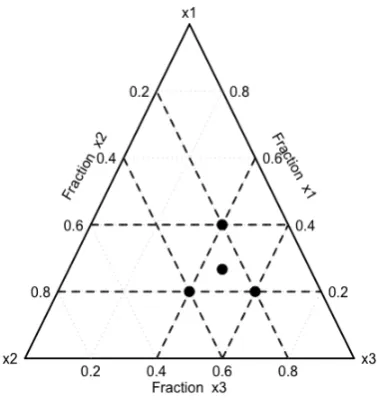
As it is easier to demonstrate and interpret a 2-dimensional simplex, we would con-sider a{3,m}Simplex-Lattice Design that is restricted by the lower boundsx1 0.4,

x2 0.2 andx3 0.2. Lawson and Willden (2016) provide us with a graphical pack-age to visualize mixture designs. Figure 1 is obtained using the packpack-age ’mixexp’ in R provided by the mentioned authors. The L-pseudocomponent is demonstrated by the smaller triangle within the original simplex. If we were to apply the transforma-tion on a higher dimensional simplex, we will obtain a smaller simplex contained inside the full simplex region, having the same dimensionality.

FIGURE2.2: The simplex region based on the constraintsx1 0.2,

x2 0.2 andx3 0.4

If the design region is bounded by one or more upper bounds, U-pseudocomponents are used. This concept can be applied by restricting at least one of the components with an upper bound less than 1 i.e. xi  Ui  1 for alli = 1, 2, . . . ,q. The range

of the U-pseudocomponents could be defined byrU = U 1, whereU = Âiq=1Ui.

Then the following transformation is used to obtain U-pseudocomponents from the full simplex

region:-x0

i = (U_Ui ₁xi) = (Ui_r xi)

U (2.32)

for alli=1, 2, . . . ,qandU >1.

We notice that the orientation of the resulting experimental region is the reverse of the original mixture space. At times, the new experimental region won’t be com-pletely contained by the original mixture space. Hence, the points inside the exper-imental region will not fall inside the original simplex as the model restriction (2.3) is not met. To check if such a situation occurs, we will see if

whereUmin is the smallest of all the upper bounds. If (2.33) is not met, we would

remove the points that fall outside the original simplex. If (2.33) is met, then we wouldn’t need to remove points as all of them will be contained inside the original simplex.

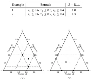
Table 1 provides two examples for the two different cases mentioned above. In Ex-ample 1, as restriction (2.33) is met, we will notice that the smaller triangle is inside the original simplex. While, in Example 2, the smaller triangle isn’t contained inside the original simplex, as the restriction is not met. Figure 2(a) illustrates the restricted simplex for Example 1, and Figure 2(b) illustrates the restricted simplex for Example 2.

TABLE2.1: Upper Bound examples

Example Bounds U Umin

1 x10.6,x2 0.3,x30.4 1.0 2 x10.6,x2 0.7,x30.4 1.3

(A) (B)

FIGURE2.3: Experimental regions for the upper bound examples, (A)

experimental region for example 1; (B) experimental region for exam-ple 2

If we compare the figures of U-pseudocomponents with that of L-pseudocomponents, we would notice that the smaller triangles are flipped in orientation, in the case of upper restrictions.

14 Chapter 2. Background

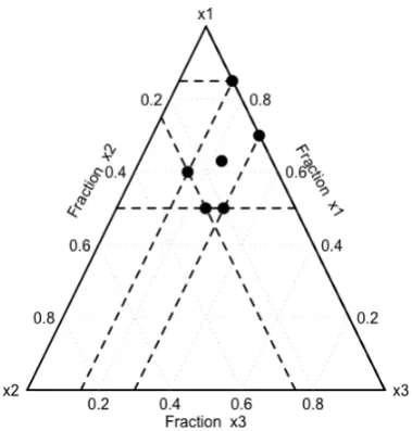
FIGURE 2.4: Experimental region for the example with both lower

and upper bounds, restricted by 0.15  x1 0.3, 0  x2  0.25 and

0.5x30.85

Now we demonstrate an example assuming that the components are restricted both ways by 0.15 _ x1  0.3, 0  x2  0.25 and 0.5  x3  0.85. The plot in Figure 2.3 was obtained by removing the points that do not fall into the intersection of the simplexes. We notice that the shape of the region in Figure 2.3 is not similar to the shape of the original simplex. We used examples with 3 components as it was easy to visualize them on a two-dimensional scale. Box and Draper (2007); Cornell (2002) provide a deeper explanation on pseudocomponents and the theory of mixture experiments.

2.6 Cholesky’s Decomposition

Cholesky’s Decomposition is a method of factorizing a matrix into a product of two triangular matrices. This techniques is widely used for simplifying matrix inversion and cutting down on the run time of computer programs that involve inverting ma-trices.

In order to implement this technique, the matrix under consideration must be Her-mitian and positive-definite i.e. a necessary and sufficient condition for a complex matrixA, to be positive definite is that the Hermitian part

AH ⌘ 1₂(A+AH)

The Cholesky decomposition of a Hermitian positive-definite matrixAcan be ob-tained by the formA = GG0_{, where Gis a lower triangular matrix with real and}

positive diagonal entries, andG0 _{is the conjugate transpose ofG. Every real-valued}

Following is the element-wise decomposition of the matrix equationA = GG0_,

us-ing Cholesky’s Decomposition

2

4AA0010 AA0111 AA0212

A20 A21 A22

3 5=

2

4GG0010 G011 00

G20 G21 G22

3 5

2

4G000 GG0111 GG0212 0 0 G22

3 5

where,

Gjj =

v u u

t_Ajj j

Â

k=0

(G2

jk)

Gij = _G1 jj Ajj

j 1

Â

k=0

GikGjk

!

Chapter 3

Literature Review

3.1 Simulation-Based Multiple Comparisons

This section discusses how the idea for constructing simulation-based critical points was introduced by Edwards and Berry (1987). They proclaimed that the renowned methods for creating simultaneous confidence intervals provided very conservative solutions in general. Hence, they laid down the foundation for simulation-based multiple-comparisons for One-Way Analysis of Variance and Analysis of Covari-ance models.

To explain this further, Edwards and Berry (1987) defined a vector of unknown model parameters b0 = (b1,b2, . . . ,bk) and their estimates ˆb0 = (bˆ1, ˆb2, . . . , ˆbk)

having a multivariate normal distribution with meanband covariance matrixs2V,

whereVis known. They defined the estimate of variance ˆs2 to be independent of

ˆ

b, such thatnsˆ2/s2 has a c2n distribution. Hence, they defined the natural pivotal quantity for a linear combinationqj =c0jbat(1 a)⇥100% confidence level. Where,

cj = (cj1,cj2, . . . ,cjk)is a vector of contrasts for allj=1, 2, . . . ,p.

W = max

1jp

8 < :

|c0

j(bˆ b)|

ˆ

sqc0_jVcj

9 =

; (3.1)

Then in theory, it must be possible to compute the upper-a percentile point, wa, satisfyingP(W > wa) = a. Hence, the exact intervals forqj for allj= 1, 2, . . . ,pare

given by

c0

jbˆ ±wa

q c0

jVcj (3.2)

Although, it was realized that the exact solution forwj can not be easily determined

numerically or analytically. Therefore, methods that could provide conservative ap-proximations forwjwere being used instead. Therefore, Edwards and Berry (1987)

suggested to substitute a random variableWa instead of the exact pivotal quantity

wa. To obtainWathe following Lemma was defined.

Lemma 1.LetW1,W2, ,Wm,Wbe independent random variables, each with the same

continuous probability distribution. For specifieda, letr= (m+1)(1 a), takea,m

such thatr is an integer. IfW(1)  W(2)  . . . , W(m) are the order statistics of W1,W2, . . . ,Wm, thenP(W >Wa) =a.

18 Chapter 3. Literature Review

is defined by the following two equations

uj = G

0_cj

q c0

jVcj

for allj=1, 2, . . . ,p (3.3)

W =max

j

( u0

jZ

Y )

(3.4)

whereZis ak dimensional vector of standard normal variates and Y is distributed aspc2/nandGis a triangular matrix obtained through Cholesky’s Decomposition

of the variance-covariance matrixV, such thatV=GG0_{. To obtainW}

a, it is required to store all themiterations of the random variableW, and arrange them in an as-cending order. Then by using Lemma 1, we haveWa =W(r), the upperapercentile

point i.e.P(W >Wa) =a.

Now the major concern that was put forward was ofWa being a random variable, had a certain amount of variability to its solution. In other words, if it was required to run the experiment again, we would obtain a different critical point. To address this concern, Edward and Berry (1987), provided another Lemma. LetGdenote the distributional function of the pivotal quantityW, andG = 1 G. Also, letG(W(r))

be the distribution of the conditional error probability. Then, Lemma 2 states the following

Lemma 2.DefineW(r)as in Lemma 1. The distribution of the conditional error

prob-abilityU = G(W(r))over repeated simulations is the beta distribution with shape

parametersm r+1 andr. That is,Uhas a density function given by ( _G(m+1)

G(m r+1)G(r)um r(1 u)r 1, 0<u<1

0, elsewhere

E(U) =a,V(U) =a(1 a)/(m+2)and for largem, this distribution is essentially normal.

Using Lemma 2, Edwards and Berry (1987) explained that witha = .05, and sim-ulation sizesm+1 = 3200, 80, 000, 320, 000, the conditional coverage probability

of simulation-based intervals will be .95_±.01, .95_±.002 and .95_±.001 in 99% of repeated generations respectively. Therefore, for a larger simulation sizem, the vari-ability in concern is almost negligible. To further demonstrate the benefits of the simulation based critical points, Edwards and Berry (1987) provided an efficiency study for a One-Way Analysis of Variance model and an Analysis of Covariance model.

3.1.1 Efficiency Study of a One-Way Layout

In the case of a One-Way Analysis problem, the fixed effects model is given by

Yij = µi+eij, for i = 1, 2, . . . ,k;j = 1, 2, . . . ,ni and the interval estimations of all

pairwise treatment differences areµi µ_i0 (1  i 6= i0  k). For such a case, the

the sample sizes are not the same, Tukey-Kramer method turns out to be conser-vative. Hence, it was discovered that the conditional probability coverage by the simulation-based method form+1=80, 000 andm+1=320, 000 was consistently

closer to 0.95 when compared to Tukey-Kramer method for cases having different sample sizes. This comparison demonstrates the reliability of the simulation based method.

3.1.2 Efficiency Study of an Analysis of Covariance Layout

Now, to prove the superiority of the simulation-based method over the traditional methods in terms of sample-size savings, Edwards and Berry (1987) conducted an ef-ficiency study for an Analysis of Covariance Model. They defined a parallel-slopes analysis of covariance setting with response Y given by Yij = µi+gcij+eij, for

i = 1, 2, . . . ,k;j = 1, 2, . . . ,ni and the interval estimations of all pairwise treatment

differences were denoted byµi µ0i (1  i 6= i0  k). The traditional methods of

multiple comparisons considered were Scheffé, Bonferroni andŠidák. To compare the performance of a simulation-based critical point with the other three methods, the concept of relative efficiency was introduced. Relative efficiency provides the approximate sample size savings at finite sample sizes by computing the ratio of the squared margins of error for the two methods under comparison, where the margin of error is the product of the critical point and the standard error. Therefore, the empirical sample size savings of method A relative to method B is 1 (wA/wB)2,

wherewAandwB are the respective critical points. Using this concept, it was

dis-covered that for cases with a smaller sample size, the simulation based critical point

(m+1 = 80, 000) was 30%, 35% and 16% more efficient than Scheffé, Bonferroni andŠidák methods respectively. But, for cases having a large enough sample size, the simulation based critical point(m+1=80, 000)was 27%, 6% and 6% more

effi-cient than Scheffé, Bonferroni andŠidák methods respectively. Therefore, Edwards and Berry (1987) claimed that the simulation-based method provided a substantial sample size savings when compared to other methods. They also mentioned that, even though the percentage savings over Bonferroni and Sidak seemed to decrease with increasingn, forn =Âk_i=1ni k 1, it had as an asymptote of a positive value;

hence, the total savings were to increase without bound asn!0.

The next section discusses the extension of this idea to general response surface de-signs.

3.2 Simulation-Based Methods for Response Surface Designs

Sa and Edwards (1993) provided the simultaneous confidence intervals for a gen-eral response surface ford(x)i.e. Expected Improvement in Mean Response w.r.t a

reference blend, where

d(x) =

k

Â

i

bixi+ k

Â

i

biix2i + k

Â

Â

i<j

bijxixj

for allx for allxsuch that x0_x=Âk

i=1x2i  R2I. Moreover, an exact solution for the

20 Chapter 3. Literature Review

adaptation was given by

d(x)₂ d(ˆ x)_±das{d(ˆ x)}for allxisuch thatx0x R2I (3.5)

such that the Scheffé critical point is da =

q

(p 1)Fa,(p 1),n, where n is the de-grees of freedom for error andpis the number of model parameters andF_a,(p 1),nis the upper 100a% critical point from the F-distribution. Sa and Edwards (1993)

pro-vided a slightly smaller simultaneous critical point by using a result from Casella and Strawderman (1980). For a 2nd_{-Order Rotatable Design, Parody and Edwards}

(2007a) provided a simulation-based critical point using the methodology formu-lated by Edwards and Berry (1987) in the case of multiple comparisons. Hence, in equation (3.5), the critical point obtained by the Scheffé adaptation(da)was replaced by the simulation based critical pointQa. This method was applied under the condi-tion that the variance-covariance matrixVwas a block diagonal matrix of the form

V= 2

4V0L V0Q 00 0 0 VCP

3

5 (3.6)

whereVL = aIk,VQ = bIk+cJk,VCP = 2bIk(k 1)/2 for constantsa,b,c; Ik,Jk being

k⇥kidentity matrix andk⇥kmatrix of ones respectively. If this structure was ob-tainable, just like in the case of a 2nd_{-order Rotatable Design, (3.5) could be replaced}

by

d(x)₂d(ˆ x)_±cas{d(ˆ x)} (3.7) whereca <

q

(p 1)Fa,(p 1),nis the Casella and Strawderman critical point.

Parody and Edwards (2007a) improved upon the work from Sa and Edwards (1993) by using a simulation-based critical point when the design was rotatable. They de-fined a natural pivotal quantity for constructing(1 a)100% simultaneous

confi-dence bounds ford(x)for allxwithin a specified distanceRI of the origin by

Q= max

0RRIxmax0x=R2 ⇢

|d(bx) d(x)_|

s{d(bx)} (3.8)

They were able to obtain a form for the numerator ofQ given by(bd(x) d(x))/s,

equal in distribution to

p

cZ00R2+pa

k

Â

i=1

Zixi+pb k

Â

i=1

Ziix2i +

p

2b

Â

i=1

Zijxixj (3.9)

where Zi,Zij,Zii and Z00 were defined as mutually independent standard normal random variables.

Parody and Edwards (2007a) claimed that the advantage of utilizing a 2nd_-order

rotatable design was that the standard error of the estimated(bx) was constant on spheres. Moreover, forVof the form (3.6),s{d(bx)_}/swas equal in distribution to

whereU⇠c2nindependent of theZ’s andR2 =x0x

By plugging in (3.9) and (3.10) in (3.8), the form ofQwas given by

Q= max

0RRI

1

U⇤_(R)xmax0_x=R2 (

p

cZ00R2+pa

k

Â

i=1

Zixi+

p

b

Â

i=1

Ziix2i +

p

2b

Â

i=1

Zijxixj

)

The maximization of the numerator over allxsuch thatx0_{x= R}2_{was solved by} Par-ody and Edwards (2007a), using the classic ridge analysis problem by Hoerl (1959). The critical pointQawas obtained from Lemma 1, as mentioned in the previous sec-tion and the(1 a)⇥100% simulation-based confident intervals for the estimated long term improvement were obtainable as

d(x)2d(ˆ x)±Qas{d(ˆ x)}for allxisuch thatx0xR2I (3.11)

It was also mentioned that to determine the simulation-based critical point for one-sided bounds, there wasn’t a need to take the absolute value of the numerator of

Q, making the computation relatively faster. Hence, for a one-sided bound, the simulation-based critical point was computed as

Q= max

0RRI

max x0_x=R2

⇢ bd(x) d(x)

s{d(bx)} (3.12)

Parody and Edwards (2007a) further reported their findings in an efficiency table. It was found out that the simulation-based method was 30% (approx.) more efficient than the Scheffé adaptation atk= 2. While, it was noticed that the sample size sav-ings further increased to 110% (approx.) atk=5.

The drawback of this technique was that it had some issues when dealing with re-gions of interest that were non-spherical in nature or if the model chosen was not a second-order model. Parody and Autin (2013) later developed a technique to op-timize the amount of improvement in the long-run mean response over a reference blend based on concentric simplexes through the use of pseudocomponents. This technique would be discussed in greater detail in the following section.

3.3 Confident Visualization Techniques in the analysis of

Mix-ture Experiments

As discussed in the previous section, Parody and Edwards (2007a) introduced a sim-ulation based critical point for a 2nd_{-order rotatable design. The major drawback of}

22 Chapter 3. Literature Review

> 3). The reference blend in this case, wasn’t needed to be prespecified. The visu-alization technique involved plotting the amount of improvement versus the range of the pseudocomponents applied. It also worked for any experimental region and model of choice.

The idea behind this technique was to optimise the amount of improvement in the long-run mean response based on concentric simplexes through the use of pseu-docomponents. These same ideas could be used to assess the impact of the refer-ence blend. Parody and Edwards (2007b) discussed confident visualization tech-niques for high dimensional response surfaces in great detail. They demonstrated a method for visualizing the improvement contours d(x) and simultaneous

confi-dence bounds whenk 2 using canonical and ridge analysis, with examples. This technique added much needed confidence to the identification and interpretation of ridge systems. The canonical bounds allowed for the identification of flexibility in the choice of predictor values, whereas the ridge trace bounds allowed for the identi-fication of the optimal choice of predictor values inside the experimental region. As this method wasn’t prohibitive in terms of the type of design, number of predictors, radius of inference, presence of blocks and covariates, or the form of the response surface, Parody and Autin (2013) extended this technique to the domain of mixture experiments.

By applying the ridge analysis bounds, as defined by Parody and Edwards (2007b), the confidence bands ford(x)along the optimal ridge path were given byd(bxˆs(R))±

da{s(d(bxˆs(R)))}, 0  R  RI, whereda =

q

(p 1)F_a,(p 1),nis the scheffé adapta-tion of the critical point. After definingxRas ap⇥1 vector of reference blend and b

as ap⇥1 vector of parameter values, they defined the amount of improvement over the reference blend as,

d(x xR) = (x xR)0b (3.13) then, by using equation (3.13), they obtained the standard error of the estimate of

d(x xR)as

snd(bx xR)

o =

q

ˆ

s2(x xR)0(X0X) 1(x xR) (3.14) Now, to extract the(1 a)⇥100% simultaneous confidence bands for the maximum improvement in response, the experimental region was attributed asTI, that could

be subset intol smaller regions of the same shape, denoted as Tl. This helped in

providing the following expression

max

x2Tl

d(x xR)2max

x2Tl b

d(x xR)±das

n b

d(x xR)

o

(3.15)

where da = ppFa,p,n with Fa,p,n being the upper 100a% critical point from the F-distribution withpandndegrees of freedom.

Plots of (3.15) for the maximisation across eachTl and their respective component

values against the constraint range were used to determine optimal settings. The constraint range were determined as

rD = q

Â

i=1

Parody and Autin (2014) enable us to extract a large number of points inside a sim-plex, using concentric pseudocomponents inside the simplex region. This idea aids us to optimize the simulation-based pivotal quantity, to obtain the desired critical point.

Chapter 4

Research Method

Monte Carlo Simulation methods to generate critical points and construction of si-multaneous confidence bands are evergreen topics of discussion in the field of statis-tics. Over the past few decades, works of Foutz (1981); Edwards and Berry (1987); Westfall and Young (1993); Hsu (1996);and Liu, Jamshidian, and Zhang (2004) have made immense contributions towards these topics. Most recently, Han, Liu, Bretz and Wan (2015) contributed towards computing critical points to construct exact symmetric bands for a percentile line using simulation procedures. Also, Zhoua, Zhu and Wang (2018) worked on adopting a simulation based method to construct confidence bands for a percentile hyper-plane having restricted covariates. In this section we proceed to the research method being employed to generate a critical point for a_{q, 2_}Simplex-Lattice Design.

4.1 Theory behind the Simulation-Based Method

Parody and Edwards (2007a) discussed the use of a natural pivotal quantity for con-structing (1 a)_⇥100% simultaneous confidence bounds for d(x)for a 2nd_-order

rotatable response surface. By utilizing the works of Edwards and Berry (1987), Parody and Edwards (2007a) and, Parody and Autin (2013) , we extend the idea of constructing 100% simultaneous confidence bounds for the predicted response in a

{q, 2}simplex-lattice design.

LetY(x)be the predicted response for given observations inxsuch thatxbelongs to a particular subset or L-Pseudocomponent(Tl)inside the full simplex region. Where

Tl 2 T such that, T is the set of all possible subsets considered in the full simplex

space. The pivotal quantityQis given

by:-Q=max

Tl2T maxx2Tl ⇢

|Yb(x) Y(x)_|

s{Yb(x)_} (4.1)

The exact(1 a)_⇥100% simultaneous confidence bounds forY(x)is given by

Y(x)₂Yb(x)_±qas{Yb(x)}for allxisuch thatx2Tl (4.2)

According to Edwards and Berry (1987), it is not possible to obtain a closed form solution toqa. Hence, a random variable Qa, generated by simulation techniques, will replaceqa. This would result in the confidence bounds having exact simulta-neous coverage probability (1 a). Also, if the random variable Q is simulated

independentlymtimes, and ifQ(1) Q(2) ...Q(m)are the order statistics of the

simulated values, thenQa =Q(a)will achieve this as long asaandmare chosen so

26 Chapter 4. Research Method

In order to proceed further, we first define the form ofY(x)given by

Y(x) =x0_b+x0_{Bx (4.3)}

wherex0 _{= [x1,x2, . . . ,xq],b}0 _{= [b1,b2, . . . ,bq]and}

B= 2 6 6 6 6 4

0 b12

2 · · · b21q 0 · · · b₂2q

... ...

(symm.) 0 3 7 7 7 7 5

To simplify (8), we will require further notation. Letz0 _{= [x1, . . . ,xq,x1x2, . . . ,xq 1xq]}

andg0 = [b1, . . . ,bq,b12, . . . ,b(q 1)q]. Now, we can express (8) as a linear

combina-tion given by

Y(x) =x0b+x0Bx=z0g (4.4)

In order to define the form of the numerator and the denominator of Q, we need to discuss the variance-covariance matrix(Vs2)of the parameter estimates ˆbi and ˆbij

for all(i,j) =1, 2, . . . ,q;i< j, where,

V= 

VL COVL,CP

COVL,CP VCP (4.5)

For a{q, 2}Simplex-Lattice Design,Var(bˆi) =s2/r,Cov(bˆi, ˆbij) = 2s2/r,Cov(bˆk, ˆbi) =

Cov(bˆk, ˆbij) = 0,Cov(bˆik, ˆbij) = 4s2/r andVar(bˆij) = 24s2/r,rbeing the number

of replications.

The partitioned matricesVL, COVL,CPandVCP are the variance-covariance

matri-ces of linear coefficients; combination of linear and cross-product coefficients; and cross-product coefficients respectively. These matrices have elements in the form of coefficients of s2 of the above mentioned quantities. Using (9), we discuss the

simulation of Q where the numerator can be defined as

b

Y(x) Y(x) =x0_(bˆ _{b) +x}0_{(Bˆ B)x=z}0_{(gˆ g) (4.6)}

Using (9) and (10), we can define ˆg as a least square estimator of the parameter

vectorg. Hence we can obtain the distribution of the estimator as ˆg ⇠ N(g,Vs2).

Following Edwards and Berry (1987), it is further noted that the signed s-scaled

numerator of Q, (Yb(x) Y(x))/s, is equal in distribution to z0GZ, where G is a

lower-triangular matrix obtained by the Cholesky’s Decomposition ofV given by

V = GG0 _{,Zis a standard normal vector such thatZ ⇠ N(0, 1). Hence, the scalar}

form of the numerator is given by

1

p

r ⇢ q

Â

i=1

aiZi+

Â

Â

i<j

aijZij (4.7)

whereai = xi(2xi 1), aij = 4xixj are fixed coefficients that are only dependent on

the elements ofxand are free of error. While,Zi,Zijare mutually independent

Moving on to the denominator of Q, we can easily ascertain that the least square estimate ˆghas a normal distribution with meang and varianceVs2. Moreover, ˆs2

is not dependent on ˆg. Using this property we also know thatnsˆ2/s2 ⇠c2n. Also by (9) we are able to define the denominator of Q as,

s{Yb(x)}=psˆ2z0Vz

= q

(U/n)z0_{Vz (4.8)}

Specifically, forVof the form (10),s{Yb(x)_}/sis equal in distribution to

U⇤ ₌

v u u t(U/n)

r  q

Â

i=1

a2

i +

Â

Â

i<j

a2

ij (4.9)

whereU⇠c2nindependent ofZ.

Hence by using the scalar form of the numerator and from (6) and (13) it follows that for a two-sided case, Q is equal in distribution to

Q=max

Tl2T

max x2Tl

|z0_GZ|

p

(U/n)z0_Vz (4.10)

=max

Tl2T

max x2Tl

1 U⇤ 1 p_r ( _q

Â

i=1

aiZi+

Â

Â

i<j

aijZij

)

(4.11)

=max

Tl2T

max x2Tl

8 > > > > < > > > > : (

Âq_i=1aiZi+Â Âq i<j aijZij

)

r_U

n

⇥

Âq_i=1a2

i +Â Âq i<j a

2 ij ⇤ 9 > > > > = > > > > ; (4.12)

According to Parody and Edwards (2007a), taking the absolute value of the numer-ator is not required in the case of one-sided bounds. Hence, the pivotal quantity (6) becomes

Q=max

Tl2T

max x2Tl

⇢ bY(x) Y(x)

s_{Yb(x)_} (4.13)

A function in R for constructing confidence intervals and one-sided bounds is given in the appendix.

28 Chapter 4. Research Method

The next section talks about the L-pseudocomponents technique being utilized for the simulation procedure.

4.2 Use of L-pseudocomponents

For this experiment, the use of L-pseudocomponents was essential to apply the sim-ulation method on a simplex-lattice design. To obtain the critical points based on the simulation procedure, it was required to optimize the pivotal quantity with respect to all possible points inside the simplex space. The idea of utilising con-centric triangles for ternary mixture systems was first discussed by Cornell and Khuri (1979). They used this idea for obtaining constant prediction variance for ternary mixture systems. Moreover, this idea was generalized by Hoerl (1987) to higher dimensions for the purpose of applying ridge analysis on hypersimplexes instead of hyperspheres. Goldfarb (2004a, 2004b), Piepel and Anderson (1992) , and Piepel et al. (1993a) provided variance dispersion graphs for mixture exper-iments, using concentric simplexes. Piepel et al. (1993b) also used concentric sim-plexes to analyse response surfaces having irregularly-shaped experimental regions. Guanghui Li and Chongqi Zhang (2017) discussed a method to apply the pseudo-component transformation on a set of uniform points under various settings of an optimal design. Guanghui Li and Chongqi Zhang (2018) adapted the random search algorithm to find optimal designs for mixture models having complex constraints. Borkowski and Piepel (2009) proposed number-theoretic methods to obtain space-filling uniform designs for high dimensional and multi-constrained mixture exper-iments. Lawson and Willden (2016) provided an R package to illustrate and visu-alize mixture designs having extreme vertices and edge and face centroids in mix-ture regions constrained by pseudo components. Parody and Autin (2013) favored the pseudocomponent approach to creating the points on the edge of the concentric simplexes, since the idea of pseudocomponents is well known in the mixture exper-iment realm.

Figure 4.1 demonstrates the effect of the number of points and L-pseudocomponents inside a simplex. In sub figures (A) and (B), keeping the number of pseudocompo-nents constant, the number of points on the triangle were increased. While, in sub figures (C) and (D) keeping the number of points constant, the number of pseudo-components were increased. It is observed that the larger the number of points and L-pseudocomponents, the greater was the density of the simplex, having a better coverage.

(A) (B)

(C) (D)

FIGURE4.1: Pseudocomponents and Point coverage in the Simplex

Chapter 5

Data Examples

5.1 Artificial Sweetener Experiment

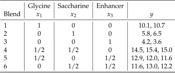
Cornell, J.A (2002) illustrated a three-component experiment consisting of three sweet-eners that were glycerine, saccharin and an enhancer. The objective of the study was to determine if the possible blends of the sweeteners could be used in a popular athletic-sports drink. The amount of sweetener was fixed at 4% of the total volume (250 mL.) of the sports drink.

In Table 1, the 3 sweeteners are given as the 3 componentsx1,x2 andx3, where the values associated with them are the design points considered on the simplex region. The responseyrepresents the "intensity of sweetness aftertaste" score for each blend. This was measured as a score on the scale of 1-30. The score of 1 being "no aftertaste" and 30 being " very extreme aftertaste". The values associated with the responsey

were computed by averaging out the scores of 20 respondents in a survey.

By fitting model (2) to the 15 data values at the six blends (1-6) of Table 1., the pa-rameter estimates are given by

ˆ

b0 = [10.40, 6.15, 3.90]

ˆ

B= 2

413.3850 13.385 10.0350 14.485 10.035 14.485 0

3 5

The MSE of the fitted model is 0.3206 with 9 df.

TABLE5.1: Data from the Artificial Sweetener Experiment

Glycine Saccharine Enhancer

Blend x1 x2 x3 y 1 1 0 0 10.1, 10.7 2 0 1 0 5.8, 6.5 3 0 0 1 4.2, 3.6 4 1/2 1/2 0 14.5, 15.4, 15.0 5 1/2 0 1/2 12.9, 12.0, 11.6 6 0 1/2 1/2 11.6, 13.0, 12.2

32 Chapter 5. Data Examples

size ofm+1 =80, 000 anda=0.05, the critical point for the simulation-based one-sided confidence bound was computed as Q0.05 = 3.244. Figure 3(a) presents the estimated improvement contours ˆd(x), whereas Figure 3(b) shows the 95%

simulta-neous upper confidence bound for the amount of improvement.

To visualize estimated maximum improvement and 95% Upper Confidence Bounds, we utilize a confident visualization technique provided by Parody and Autin (2013) which enables us to observe and interpret the contours of the entire surface inside the simplex region. In Figure 3(a), we can see that there is indeed a region that yields positive values for the estimated improvement. Any of the component values inside the contour with response value 0 will meet this requirement. The improvement re-gion is closer to the left vertex, proving a better response than the control settings (centroid). While, in Figure 3(b), we observe that the region that yields positive val-ues of improvement is larger than that of the estimated maximum improvement. In fact, there is also a region where the 95% Upper Confidence bounds for estimated improvement are greater than 0.5. Having a minimization problem, based on figure 3, we observe that the minimum response is obtained towards thex3vertex. Hence, the minimum estimated response is found out to be 3.9 corresponding to the design point(0, 0, 1).

FIGURE5.1: Artificial Sweetner Example; (a) Estimated Improvement

contours relative to the centroid; (b) simulation-based lower 95% si-multaneous confidence bounds. The region inside the zero contour

indicates improvement over the control settings

In this example, we observe that the squared simulation-based critical pointQ2 0.05 = 10.524 is approximately half in magnitude to the squared critical point obtained from the Scheffé method,d2

ratio. Hence we have(d2

0.05/Q0.05)2 1 = 0.92. This would mean that to make the scheffé method equally precise to the simulation-based method, it will be required to increase the sample size by 92%. 2

5.2 Tropical Beverage Experiment

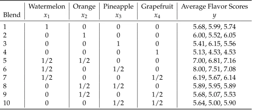
The second example is also an experiment discussed by Cornell, J.A (2002). In this experiment, a tropical beverage was formulated by blending the juices of water-melon(x1), orange(x2), pineapple(x3), and grapefruit(x4). The response measured in this study is the average flavor score (based on a scale of 1-9) considering 40 sam-ples of each blend having 3 replicates each. The goal of this study is to maximize the average flavor score of the tropical beverage. Each of the fruit flavors were con-sidered as pure blends as well as having binary combinations with the other three flavors.

TABLE5.2: Data from the Tropical Beverage Experiment

Watermelon Orange Pineapple Grapefruit Average Flavor Scores Blend x1 x2 x3 x4 y

1 1 0 0 0 5.68, 5.99, 5.74 2 0 1 0 0 6.00, 5.52, 6.05 3 0 0 1 0 5.41, 6.15, 5.56 4 0 0 0 1 5.13, 4.53, 4.53 5 1/2 1/2 0 0 7.00, 6.81, 7.16 6 1/2 0 1/2 0 8.00, 7.51, 7.08 7 1/2 0 0 1/2 6.19, 5.67, 6.14 8 0 1/2 1/2 0 5.89, 5.95, 5.89 9 0 1/2 0 1/2 5.68, 5.07, 5.53 10 0 0 1/2 1/2 5.64, 5.00, 5.90

By fitting model (2) to the 10 data values at the six blends (1-10) of Table 2., the parameter estimates are given by

ˆ

b0 = [5.80, 5.85, 5.71, 4.73]

ˆ

B= 2 6 6 4

0 2.32 3.55 1.46 2.32 0 0.26 0.27 3.55 0.26 0 0.59 1.46 0.27 0.59 0

3 7 7 5

The MSE of the fitted model is 0.1023 with 20 df.

We assume that the objective of the study is to see if any improvement in the score for the reference blend can be made over the average flavor scores. The ref-erence blend was set as the centroid for the Tropical Beverage example i.e. x0

R =

(0.25, 0.25, 0.25, 0.25). The estimated response for the reference blend is ˆy(xR) =

34 Chapter 5. Data Examples

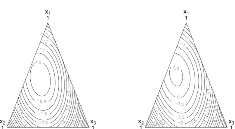
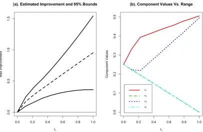
FIGURE 5.2: Tropical Beverage Example; (a) 95% simultaneous bounds for the amount of improvement over the control along the es-timated optimal component path using the simulation-based method

(4); (b) estimated optimal component path

Based on Figure 4(a), the estimated response for the Tropical Beverage experiment is maximized at rL = 1. This corresponds to the edge of the experimental

re-gion. At this range, the estimated amount of improvement over the reference blend is roughly 1.0. Based on Figure 7(b), the blend where the maximum is found is

(0.505, 0, 0.495, 0). The lower bound for improvement for the top flavor score at this

blend is 0.36. The fact that the entire lower bound region is made up of positive val-ues indicates that there is indeed some possible improvement in top contour score over the reference blend.

In this example, havingq = 4, we see more improvement in efficiency when we

compare the squared simulation-based critical pointQ2

0.05 = 10.95 with the Scheffé adaptation given by Sa and Edwards (1993),d2

Chapter 6

Discussion and Conclusions

Based on the examples provided in the previous section, the simulation-based method defined in section 3 yields substantially narrower bounds than the Sa and Edwards (1993) adaptation of the Scheffé method. In this section, an efficiency study is con-ducted to ascertain the amount of sample size savings by using the simulation-based method for confidence intervals. The study compared critical points forq = 3 5,

a= 0.05 andr = 2, 3, 4, 5, 7,•. Simplex lattice designs withm= 2 were utilized in

the efficiency study, for all the values ofqandrmentioned above. Table 3 provides the sample-size savings of the two-sided simulation-based method over the Sa and Edwards adaptation of the Scheffé method.

TABLE6.1: Approximate sample-size savings, two-sided

simulation-based method to the Sa and Edwards (1993) adaptation of the Scheffé method ata=0.05.

q

r 3 4 5

2 50.1% 78.8% 108.3% 3 45.9% 75.4% 97.4% 4 44.9% 72.9% 95.8% 5 44.8% 73.3% 93.9% 7 43.6% 71.0% 94.0%

• 43.6% 69.5% 92.3%

From Table 3, we observe an improvement of more than 100% over the Sa and Ed-wards adaptation of the Scheffé method by using this simulation-based method when we set the number of factor to be large enough. Even for a small number of factors , the sample size savings is still considerable, at approximately 50%. As we increase the number of pure blends (q), the sample size savings have greater im-provement over the Scheffé method. Forq = 5, the sample size savings are more

than double for using the simulation-based critical point.

36 Chapter 6. Discussion and Conclusions

Bibliography

[1] Casella, G. and Strawderman, W.E. (1980) ‘Confidence bands for linear regres-sion with restricted predictor variables’,Journal of the American Statistical Associa-tionVol. 75, No. 372, pp.862–868.

[2] Cornell, J.A. (2002)Experiments with Mixtures Designs, Models, and the Analysis of Mixture Data, 3rd ed., Wiley & Sons, New York.

[3] Cornell, J.A. and Khuri, A.I. (1979) ‘Obtaining constant prediction variance on concentric triangles for ternary mixture systems’, Technometrics , Vol. 21, No. 2, pp.147–157.

[4] Edwards, D. and Berry, J. J. (1987). The efficiency of simulation-based multiple comparisons.Bi