ROBUST SEMI-EXPLICIT MODEL PREDICTIVE CONTROL FOR HYBRID AUTOMATA Yan Pang∗,Hao Xia∗,Michael P. Spathopoulos∗
∗University of Strathclyde, Glasgow, G1 1QE, U.K. {yan.pang, hao.xia, michael.spathopoulos}@strath.ac.uk
Abstract: In this paper we propose an on-line design technique for the target control problem of hybrid automata. First, we compute off-line the shortest path, which has the minimum discrete cost, from an initial state to the given target set. Next, we derive a controller which successfully drives the system from the initial state to the target set while minimizing a cost function. The (robust) model predictive control (MPC) technique is used when the current state is not within a guard set, otherwise the (robust) mixed-integer predictive control (MIPC) technique is employed. An on-line, semi-explicit control algorithm is derived by combining the two techniques and applied on a high-speed and energy-saving control problem of the CPU processing.
1. INTRODUCTION
In this paper, a computationally efficient solu-tion is presented for the supervisory target con-trol of hybrid automata (Trontis and Spathopou-los, 2003). The controller design can be considered as a two stage optimization. At the first stage, for any given initial state, we solve a high priority optimization problem which minimizes the total discrete transition cost to the target set. This is cast as a reachability problem from a given initial set to a target set. With this reachability problem solved, the initial set can be partitioned into a number of disjoint subsets, and any state contained in a given subset will have the same discrete switching path (weighted shortest path) of the minimized discrete transition cost. At the second stage, for a given initial state, a hybrid controller can be derived based on the results from stage one. The design is formulated as a low priority optimization problem which min-imizes a continuous transition performance index subject to the constraint that the weighted short-est path will be followed. Due to the constraints imposed on the system state and control input, a constrained optimization needs to be solved. A hybrid controller is calculated on-line using model predictive control (MPC) techniques.
Considering the high computational complex-ity of the MPC on-line algorithm presented in (Bemporad et al., 1999), we formulate a semi-explicit(sub-optimal) method that reduces the computational burden. For this, we remove the on-line choices for the switching part, by selecting the shortest discrete path offline. It is then shown that
the shortest path can be used to derive a semi-explicit algorithm for hybrid automata. The de-sign proposed in this paper is computationally ef-ficient due to the fact that the global optimization problem has been decomposed into several consec-utive local optimization problems. However, the price to be paid for the computational saving is that the result is sub-optimal.
The rest of the paper is organized as follows. In the next section the basic definitions and concepts related to hybrid automata are given. The MPC and MIPC problems are stated and addressed in section 3, In section 4, a semi-explicit algorithm for the problem stated is derived. In section 5, we discuss the effect of bounded disturbances and how the nominal design can be applied in the presence of these disturbances. A CPU application of the algorithm is given in section 6.
2. MODELLING AND PROBLEM FORMULATION
2.1 Hybrid automaton
The discrete-time hybrid automaton used in this paper is defined as follows:
Definition 1. (Pang and Spathopoulos, 2005), A linear discrete-time hybrid automaton is a collection A = (Q, X, f, U, D,Σ, Inv, E, G, c) where Q={q1, ..., qN} is a set of discrete states;
X ⊆Rnis the continuous state space;f :Q×X×
U → 2X assigns every discrete state a Lipschitz continuous evolution function which is described by the linear difference equation (1):
The control inputu(t)∈Uand disturbanced(t)∈
D that both contain the origin as an interior point. Σ is the set of discrete inputs; let ǫ ∈ Σ denote the situation where no discrete command is issued; Inv : Q → 2X assigns each q ∈ Q an invariant set; E ⊆ Q×Σ×Q is a collection of discrete transitions; G : E → 2X assigns each
e = (q, σ, q′) ∈ E a guard; c : (Q×Q) → R+
assigns a positive cost to each transition.
All the sets involved above are considered as polytopes. The guard set Gq,q′(σ) is the subset
of the state space where the system can switch from location q to q′. The moment at which the transition takes place is a design variable. An external system (controller) orders an appropriate discrete input when a certain condition, subject to design, is satisfied.
Definition 2. A hybrid controller is a map: C :
Q×X →2Σ×U. The controller issues both discrete inputs Cd(q(t), x(t))∈2Σ and continuous inputs Cc(q(t), x(t))∈2U.
2.2 Problem Statement
Let Π ={π} denote the set of all discrete paths fromq0 toqF:
Π ={π|∃σ,∃N ∈N, j= 0, ..., N−1, qN =qF :
ej = (qj, σ, qj+1)∈E∧π= (q0, ..., qN)} Essentially, the discrete paths are derived by ab-stracting the continuous dynamics awayi.e. con-sidering reachability on the discrete graph. Let
l(π) be the number of discrete transitions in a pathπ∈Π. Therefore,π= (qπ
0, q1π, ..., qlπ(π)), with qπ
0 = q0, qlπ(π) = qF and the cost of path π is defined as:c(π) =Pl(π)
i=1c(qi−π 1, qπi). This function represents the transition cost alongπfrom an ini-tial state (q0, x0) to a final state (q(tf), x(tf))∈F. Given a hybrid automatonAand a target setF = (qF, XF), for a state (q0, x0), the control problem
defined here can be cast as follows: Design the sequence of control inputs such that all trajec-tories will reach the target set while minimizing associated cost functions. This is formulated in two steps:
(1) find the shortest discrete path with the min-imal discrete costc(π);
(2) compute optimal (continuous and discrete) control inputs for each discrete state (loca-tion) on-line. Here optimality is addressed locally and therefore the overall design is suboptimal.
For the first step, we utilize a generalization of Dijkstra’s shortest path algorithm on weighted graphs (Martinset al., 1998), and find the shortest path with the minimum costc(π) fromq0 toqF.
For the second step, if the current state is not in the desired guard set, then the standard MPC method is employed to drive the current state to the guard set where the system may be switched to the next discrete state along the path π. On the other hand, if the current state has already reached the guard set, then the MIPC method is used to drive the current state to the next guard set along the path π. This procedure is repeated until the target set is reached without violating any constraint.
3. MPC AND MIPC PROBLEMS
In this section, it is assumed that there is no additive disturbance in linear discrete-time model defined in equation 1.
3.1 The Model Predictive Control (MPC) Problem
For the shortest path π, the aim is to com-pute a suboptimal controller which successfully drives the system from (q0, x0) into (qF, XF). Let
π= (qπ
0, qπ1, ..., qπl(π)) be the path, and G
π qi,qi+1 =
{x|Cπ
ix ≤ hπi} be the transition guards from discrete stateqπ
i toqπi+1, withi= 0,1, ..., l(π)−1,
where Cπ
i ∈ Rnc×n, hiπ ∈ Rnc. Also, let XF = {x|CFx ≤ hF}, with CF ∈ Rnf×n, hF ∈ Rnf. Given a state x(t) ∈ Inv(qπ
i), we define the fol-lowing optimal control problem:
Problem 1
First define the following cost function:
Ji(UtN−1, x(t)) =:ω1·kx(t+N|t)−Tikp+ N−1
X
k=0 ω2
·kx(t+k|t)−Tikp+ N−1
X
k=0
ω3· ku(t+k|t)−uekp
The factorsω1, ω2, ω3∈Rare appropriate weights
for the contributions of these three terms. Also,
UtN−1 =: [uT(t+ 0|t), uT(t+ 1|t), ..., uT(t+N− 1|t)]T. At each time t, x(t+k|t) and u(t+k|t) denote the predicted state and input at timet+k. kx(t+k|t)−Tikp describes the distance between the current state and (the nearest boundary) of the guard (target) set:
Ti=
½
Gπqi,qi+1 if i∈ {0,1, ..., l(π)−1}
XF if i=l(π) (2)
with a normk · kp,p=∞,2,1.ku(t+k|t)−uekp contains the deviation ofu(t+k|t) from a reference inputue.N is the prediction horizon.
The finite-time optimal control problem is defined as:
min UN−1
t
Ji(UtN−1, x(t))
s.t.
x(t+k+ 1|t) =
Aqπ
ix(t+k|t) +Bqiπu(t+k|t) +cqπi u(t+k|t)∈U
The main idea of predictive control is to use the model of the plant to predict the future evolution of the system. Based on this prediction, at each time steptthe controller selects a sequence of future command inputs through an on-line optimization procedure, which aims at minimizing the distance from the current state to the target set, and enforces fulfillment of the constraints. Only the first sample of the optimal sequence is actually applied to the plant at time t. At time
t+ 1, a new sequence is evaluated to replace the previous one. This on-line “re-planning” provides the desired feedback control feature.
3.2 The Mixed Integer Predictive Control (MIPC) Problem
Once the statex(t) is driven to a guard setGπ qi,qi+1
using MPC, it is up to the discrete controller to decide whether to let it idle in state qi or switch to the next state qi+1. To design the local
opti-mal discrete controller, the logical decisions and the transition structure of Aare expressed using relations of binary variables, and the solution is then determined by Mixed Integer Programming (MIP).
The dynamics at t are determined by the cur-rent discrete state and input. Let |Q| denote the number of discrete states ofA. We introduce |Q| binary variables defined as
λi(t) =
½
1 if q(t) =qi
0 otherwise i∈ {1, ...,|Q|}
It is clear that: |Q|
X
i=1
λi(t) = 1 (3)
Under the assumption that the guard setGπ qi,qi+1
has no intersection with another guard setGπ qi,qj, j 6= i + 1 along the path, we have for state
x(t)∈Gπ
qi,qi+1 that:
λi(t) +λi+1(t) = 1 (4)
where λi(t) and λi+1(t) are the binary variables
associated with the discrete states qπ
i and qπi+1
respectively.
The following optimal control problem is solved for the statex(t)∈Gπ
qi,qi+1which can be observed
by the system. Problem 2
Define the cost function
Ji′(U N′−1
t , x(t)) =:ω1·kx(t+N′|t)−Ti+1kp+ω2·
N′−1 X
k=0
kx(t+k|t)−Ti+1kp+ω3·
N′−1 X
k=0
ku(t+k|t)−uekp
where N′ is the prediction horizon and consider the finite-time optimal control problem
min UN′ −1
t
Ji′(U N′−1
t , x(t)) (5)
s.t
x(t+k+ 1|t) =λi(t+k|t)[Aqπ
ix(t+k|t)+ Bqπ
iu(t+k|t) +cq π
i] +λi+1(t+k|t)[Aq π i+1 x(t+k|t) +Bqπ
i+1u(t+k|t) +cq
π i+1] u(t+k|t)∈U
x(t+k|t)∈Gπqi,qi+1
λi(t+k|t), λi+1(t+k|t)∈ {0,1} λi(t+k|t) +λi+1(t+k|t) = 1 λi(t+k|t)−λi(t+k−1|t)≤0
(6) It should be noted that the set Ti+1 is different
for the setTi in problem 1 as:
Ti+1= ½
Gπqi+1,qi+2 if i∈ {0,1, ..., l(π)−2} XF if i=l(π)−1
The constraintλi(t+k|t)−λi(t+k−1|t)≤0 for all k = 1, . . . , N′ in the last line of equation (6) guarantees that there is only one jump fromqπi to
qπ
i+1. For any l = 0, ..., N′, if λi(t+l|t) = 0, the
system is switched to the next discrete location
qπ
i+1 since it is impossible to have another l′ > l
such thatλi(t+l′|t) = 1.
2. The computational tools of MPC are linear pro-gramming (LP) or quadratic programing (QP), while the tools for MIPC are mixed integer linear programming (MILP) or mixed integer quadratic programming (MIQP), see (Pang et al., 2005) for more details.
4. A SEMI-EXPLICIT ALGORITHM
Given a discrete path π = (q0, q1, ..., ql(π) = qF) and an initial state (q0, x0), the following online
predictive control algorithm derives a controlled trajectory from (q0, x0) to the target set :
Algorithm 1. (A semi-explicit algorithm). 1.t= 0, i= 0, x(0) =x0;
2.whilei≤l(π)−1do; 3. if x(t)∈Gπ
qiqi+1;
4. solve problem 2; 5. if λ∗
i(t) = 1∧x(t+ 1)∈Gπqiqi+1;
6. C∗(q(t), x(t)) = (ǫ, u∗
t(0)),t:=t+ 1; go to 3
7. else
8. C∗(q(t), x(t)) = (σi,i+1, u∗t(0));
t:=t+ 1;i:=i+ 1; go to 2
9. end
10. else
11. solve problem 1;C∗(q(t), x(t)) =(ǫ, u∗t(0));
t:=t+ 1; go to 3 12.end while
13.whilex(t)6∈XF do;
14. solve problem 1;C∗(q(t), x(t)) = (ǫ, u∗ t(0));
t:=t+ 1 15.end while
while loop terminates when x(t) ∈ XF. In the firstwhile, the algorithm first checks whether the continuous statex(t) is in the guard set or not. If yes, it solves the MIPC problem 2. The solution of problem 2. provides both the continuous and discrete inputs. When a discrete switching occurs, the index i is increased by one and the system evolves in the new discrete state. On the other hand, if the continuous state is outside the guard set, the algorithm solves the MPC problem 1 and calculates the continuous input which optimally drives the system to the guard (target) set.
5. ROBUST MPC AND MIPC
In the previous sections, it is assumed that there is no additive disturbance in the continuous dynam-ics. Since MPC and MIPC are both receding hori-zonstate feedback laws, the inherent robustness of deterministic MPC and MIPC applied to nominal system is usually enough if the disturbance is sufficiently small (Scokaert and Rawlings, 1995). On the other hand, it is well known that the action of a bounded disturbance can destabilize a predictive controller which is stabilized for the nominal case. A straightforward solution is to treat the disturbance explicitly and carry out a min-max optimization as proposed in (Scokaert and Mayne, 1998). However, there are two ma-jor drawbacks associated with this “worst-case” formulation. The first is that the resulting opti-mization procedure is computationally expensive and the second is that the optimizing performance for the “worst-case” disturbance represents an unrealistic scenario and may yield poor perfor-mance whenever the disturbance realization gets close to zero. For the above reasons, a more sen-sible approach is to minimize the nominal per-formance index while imposing constraint fulfill-ment for all admissible disturbances. This idea has been pursued in (Chisci et al., 2001; Langson et al., 2004; Mayne et al., 2005). In this paper, we will adapt a similar strategy, so that all results introduced before can be used.
Feedback model predictive control in which the decision variable is a policy c, was advocated in (Lee and Yu.Z., 2005; Scokaert and Mayne, 1998). Thepolicyis a sequence{µ0(·), µ1(·), . . . , µN−1(·)}
of control laws. Determination of a control policy is usually prohibitively difficult, as first introduced in (Lee and Kouvaritakis, 2000). Thus, a sub-optimal control policy in whichµi(x) =vi+Kx will be employed here. This state feedback law transforms the decision variable from a policy to a sequence of control actions {v0, v1, . . . , vN−1}.
The inherent feedback via the time-invariant K
reduces the spread of trajectories due to distur-bance and it is often very effective.
Before introducing the main result of this section, a few set notations need to be introduced. Given two setsA, B, thenA⊕B,{a+b|a∈A, b∈B} (set addition) and A⊖B ,{a|a⊕B⊆A} (set subtraction).
For the discrete time system defined in (1), its corresponding nominal model is defined by
x(t+ 1) =Ax(t) +Bu(t) (7)
For the nominal model (7) and an initial condition ¯
x0, let ¯u,{¯u0, . . . ,¯uN−1}be the optimal control
sequence for the cost function. By applying ¯u to (7), the optimal nominal state trajectory can be obtained as ¯x = {¯x0,x¯1, . . . ,x¯N). For the perturbed plant (1), the feedback policy c is defined as:
µi(x,x¯i,u¯i),u¯i+K(x−x¯i) = (¯ui−Kx¯i) +Kx,
i= 0,1, . . . , N−1 (8) Suppose the sequences {xi} and {ui} are the so-lutions of the perturbed system (1) with feedback policyc,i.e.{xi} and{ui}satisfy:
xi+1=Axi+Bui+di
ui= ¯ui+K(x(i)−x¯(i))
with initial conditionx0= ¯x0. A simple inductive
argument yields
xi∈x¯i+ i−1 X
j=0
AjKD i= 1, . . . , N (9)
ui∈u¯i+K i−1 X
j=0
AjKD i= 1, . . . , N −1 (10)
withAK=A+BK andPdenoting set addition. Clearly, the feasibility of the feedback policy c
depends on whetherxi andui satisfy the original state and control constraint respectively. Based on equations (9) and (10), with initial state x0∈X,
in order to guarantee the feasibility ofc, (¯x,u¯) has to satisfy tighter constraints:
¯
xi∈Inv∗(q)⊖ i−1 X
j=0
AjKD, i= 1, . . . , N(11)
¯
u0∈U, u¯i∈U⊖K i−1 X
j=0
AjKD, i= 1, . . . , N−1(12)
From the above two equations, it is clear that the state feedback gain K should be chosen such thatPi−1
j=0A
j KD, K
Pi−1
j=0A
j
KD, i= 1, . . . , N− 1 are minimized. A computational technique for the minimum over approximation of these sets has been presented in (Rakovicet al., 2005).
CPU Cooling Fan
Buffer
w
v
p r
Fig. 1. The CPU model
6. CPU PROCESSING CONTROL
In this section, the above results are applied on the CPU processing control problem (Azuma and Imura, 2003). In order to realize the high-speed and energy-saving computing more effectively, we model the system as a hybrid automaton and apply the semi-explicit algorithm 1 to this system. The state of system when a sufficiently long time has passed after booting the system is defined as equilibrium state of this model, and define the output of the temperature sensor equipped on the motherboard as the CPU temperature. Then from some experimental results, the dynamical behaviors of this model around equilibrium state are given as follows: (a) the time variation of the amount of CPU tasks in the buffer proportionally decreases as clock frequency increases, and (b) the time variation of CPU temperature proportionally increases as the clock frequency increases and the angular velocity of cooling fan decreases.
Thus the state equations of this model around the equilibrium state are expressed as follows:
˙
π=−K1c
˙
ρ=−K2ρ+K3c−K4ω
˙
ω=−K5ω+K6v
(13)
whereπ∈R, ρ∈R, andω∈Rare the deviations
of the amount of CPU tasks in the buffer, the CPU temperature and angular velocity of a cooling fan from the equilibrium state, respectively, andc∈R
and v ∈ Rare deviations of clock frequency and
the voltage input of a cooling fan from equilibrium input, respectively. The first and second equations express the dynamics (a) and (b), while the third equation is the dynamics of the DC motor of fan.
Let c and v can be switched according to the values of π and ρ at the switching times. The policy is that
• the voltagevof cooling fan is the only control input in the usual mode (q1);
• the clock frequency c is the only control if the amount of CPU tasks is large but CPU temperature is not so high that is called busy mode (q3);
• bothcand vare used as control inputs only in an emergency mode (q2).
Let x= [π, ρ, ω]T and u= [c, v]T be the contin-uous state and control input. The parameters in
Table 1. Continuous dynamics.
State Dynamics( ˙x=) Input Invariant
q1
·0 0 0
0 −0.05 −0.5 0 0 −3
¸
x+
·0 0
0 0 0 0.5
¸
u c= 0 v∈[−10,10]
−10≤π≤3
−10≤ρ≤10
−10≤ω≤10
q2
·0 0 0
0 −0.05 −0.5
0 0 −3
¸
x+
·−1 0
0.1 0
0 0.5 ¸
uc∈[−5,5] v∈[−10,10]
π≤10
ρ≤10
π+ρ≥10
−10≤ω≤10
q3
·0 0 0
0 −0.05 −0.5
0 0 −3
¸
x+ ·−1 0
0.1 0
0 0
¸
u c∈[−5,5] v= 0
0≤π≤10
−10≤ρ≤7
−10≤ω≤10
1
q q2 q3 q1
12
[image:5.595.306.536.77.380.2]G G23 G31
Fig. 2. The discrete pathπ.
0 5 10 15 20 25
−10 −8 −6 −4 −2 0 2 4 6 8 10
x
1
x
2
[image:5.595.327.509.445.546.2]x3
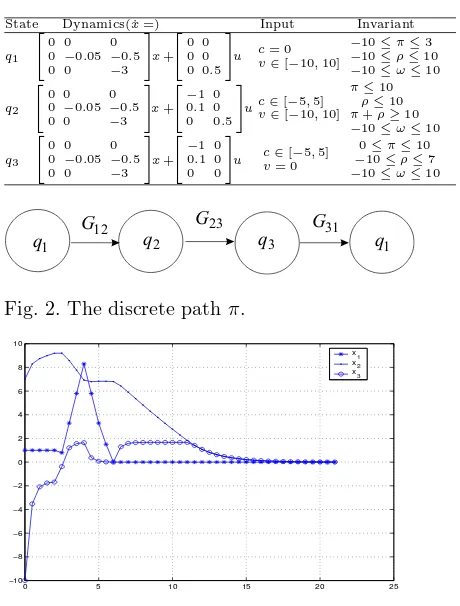
Fig. 3. Trajectories ofx1(t), x2(t) andx3(t).
each location are shown in Table 1. The discrete path considered in this example is described in figure 2. where the guard sets are:
G12(σ12) = ½
x ¯ ¯ ¯ ¯
·−1 −1 0
1 0 0 0 1 0
¸ x≤
·−10
3 10
¸ ¾
G23(σ23) = ½
x ¯ ¯ ¯ ¯
·−1 −1 0
1 0 0 0 1 0
¸ x≤
·−10
10 7
¸ ¾
G31(σ31) = (
x ¯ ¯ ¯ ¯ ¯
" 1 0 0
−1 0 0
0 1 0 0 −1 0
#
x≤
"3
0 7 10
# )
The initial and target states are (q1,[1,7,−10]T)
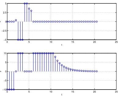
and (q1,[0,0,0]T) and the equilibrium input is ue = [0,0]T. Applying the algorithm 1 on the discretized automaton with Ts = 0.5s, we have the simulation results shown in figure 3. The trajectory projected on π−ρ space is shown in figure 4. The optimal input of the controller is depicted in figures 5 and 6.The execution time on a Pentium 1GHz with 256MB RAM is 3.435 s.
7. CONCLUSIONS
−10 −8 −6 −4 −2 0 2 4 6 8 10 −10
−8 −6 −4 −2 0 2 4 6 8 10
π
ρ
G
31
G12
G23
Inv(q
1)
Inv(q2)
Inv(q
3)
x
f
x
[image:6.595.74.262.69.314.2]0
Fig. 4. The trajectory onπ−ρspace.
0 5 10 15 20 25
0 1 2 3 4
t
q
σ12 σ23 σ
[image:6.595.75.268.354.511.2]31
Fig. 5. Discrete states along the optimal trajectory and optimal discrete inputs.
0 5 10 15 20 25
−10 −5 0 5 10
t
v
0 5 10 15 20 25
−5 −2.5 0 2.5 5
t
c
Fig. 6. Optimal continuous inputs.
ndeterminism. Algorithm 1 reduces the on-line computation by deriving off on-line the shortest discrete path. In addition, the on-line controller avoids non-determinism by supplying a sequence of optimal control inputs, instead of sets of control inputs as in (Pang and Spathopoulos, 2005). MPC and MIPC of hybrid systems has been extended to systems in the face of persistent disturbances. This is achieved by imposing tighter state and control constraints to the nominal system. Then, the feedback predictive controller, based on the nominal state and control trajectories, provides a suboptimal solution to the target control prob-lem.
8. REFERENCES
Azuma, S. and J. Imura (2003). Optimal control of sampled-data piecewise affine systems and its application to cpu processing control. In:
Proceedings of the 42nd IEEE Conference on Decision and Control. Maui,Hawaii USA. Bemporad, A., D. Mignone and M. Morari
(1999). Control of systems integrating log-ical, dynamics, and constraints. Automatica
35(3), 407–427.
Chisci, L., J.A. Rossiter and G. Zappa (2001). Sys-tems with persistent disturbances: predictive control with restricted constraints. Automat-ica37, 1019–1028.
Langson, W., I. Chryssochoos, S.V. Rakovic and D.Q. Mayne (2004). Robust model predictive control using tubes.Automatica40, 125–133. Lee, J.H. and Yu.Z. (2005). Worst-case formu-lations of model predictive control for sys-tems with bounded parameter. Automatica
41, 125–133.
Lee, Y.I. and B. Kouvaritakis (2000). Robust re-ceding horizon control for systems with un-certain dynamics and input saturation. Auto-matica36, 1497–1504.
Martins, E., M. Pascoal and J. Dos Santos (1998). The k shortest paths problem. Technical re-port. Department of Mathematics, Coimbra University. Portugal.
Mayne, D.Q., M.M. Seron and S.V. Rakovic (2005). Robust model predictive control of constrained linear system with bounded dis-turbances.Automatica 41, 125–133.
Pang, Y. and M.P. Spathopoulos (2005). Time-optimal control for discrete-time hybrid au-tomata. International Journal of Control
78(11), 847–863.
Pang, Y., M. P. Spathopoulos and J. Raisch (2005). On suboptimal control design for hybrid automata using predictive control techniques. In: Proceedings of the 16th IFAC World Congress on Automatic Control. Prague.
Rakovic, S.V., E.C. Kerrigan, K.I. Kouramas and D.Q. Mayne (2005). Invariant approxima-tions of the minimal robust positively invari-ant set. IEEE Trans. on Automatic Control
50(3), 406–410.
Scokaert, P.O.M. and D.Q. Mayne (1998). Min-max feedback model predictive control for constrained linear systems. IEEE Trans. on Automatic Control43, 1136–1142.
Scokaert, P.O.M. and J.B. Rawlings (1995). Sta-bility of model predictive control under per-turbantions. In:Proceedings of IFAC sympo-sium on nonlinear control systetms design. Lake Taboe, CA.