A hybrid ant algorithm for scheduling independent jobs in heterogeneous
computing environments
Graham Ritchie and John Levine
Centre for Intelligent Systems and their Applications Department of Computer and Information Sciences School of Informatics, University of Edinburgh University of Strathclyde
Appleton Tower, Crichton Street, Edinburgh, EH8 9LE Livingstone Tower, 26 Richmond Street, Glasgow, G1 1XH
[email protected] [email protected]
Abstract
The efficient scheduling of independent computational jobs in a heterogeneous computing (HC) environment is an im-portant problem in domains such as grid computing. Finding optimal schedules for such an environment is (in general) an NP-hard problem, and so heuristic approaches must be used. In this paper we describe an ant colony optimisation (ACO) algorithm that, when combined with local and tabu search, can find shorter schedules on benchmark problems than other techniques found in the literature.
Introduction & Motivation
The efficient scheduling of independent computational jobs in a heterogeneous computing (HC) environment such as a computational grid is clearly important if good use is to be made of such a valuable resource. However, finding optimal schedules in such a system has been shown, in general, to be NP-hard (it is a generalised reformulation of SS8 from (Garey and Johnson, 1979)).
Static scheduling algorithms can be used in such a system for several different requirements (Braun et al., 2001). The first, and most common, is for planning an efficient sched-ule for some set of jobs that are to be run at some time in the future, and to work out if sufficient time or computa-tional resources are available to complete the run a priori. Static scheduling may also be useful for analysis of hetero-geneous computing systems, to work out the effect that los-ing (or gainlos-ing) a particular piece of hardware, or some sub-network of a grid for example, will have. Static scheduling techniques can also be used to evaluate the performance of a dynamic scheduling system after it has run, to check how effectively the system is using the resources available.
The ant colony optimisation (ACO) meta-heuristic was first described by Dorigo (Dorigo, 1992) as a technique to solve the travelling salesman problem, and was inspired by the ability of real ant colonies to efficiently organ-ise the foraging behaviour of the colony using external chemical pheromone trails as a means of communication. ACO algorithms have since been widely employed on many other combinatorial optimisation problems (see (Dorigo and St¨utzle, 2002) for a review), including several domains re-lated to the problem in hand, such as bin packing (Levine
Copyright c 2004, American Association for Artificial Intelli-gence (www.aaai.org). All rights reserved.
and Ducatelle, 2003) and job shop scheduling (van der Zwaan and Marques, 1999), but ACO has not previously been applied to finding good job schedules in an HC en-vironment.
Simulation Model
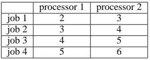
Real-world HC systems, such as a computational grid, are complex combinations of hardware, software and network components and so it is often hard to make fair comparisons of the different techniques that are being used on various dif-ferent systems. To address this problem (Braun et al., 2001) describes a benchmark simulation model for comparison of static scheduling algorithms for HC environments. They define the notion of a metatask as a collection of indepen-dent jobs with no inter-job dependencies, and the goal of a scheduling algorithm is to minimise the total execution time of the metatask. As the scheduling is performed statically all necessary information about the jobs in the metatask and processors in the system is assumed to be available a priori. Essentially, the expected running time of each individual job on each processor must be known, and this information can be stored in an ‘expected time to compute’ (ETC) matrix. Of course, in a real scheduler, there may be some difference be-tween the expected time to compute and the real time taken to complete a job, but for this paper we assume that the value in the ETC matrix is the running time of the job and we leave it to further work to test the scheduler in a more realistic en-vironment. A row in an ETC matrix contains the ETC for a single job on each of the available processors, and so any ETC matrix will haven×mentries, wherenis the number of jobs andmis the number of processors. A simple exam-ple ETC matrix with details for 4 jobs and 2 processors is given in table 1.
In any real heterogeneous computing system the running time of a particular job is not the only factor that must be taken into consideration when allocating jobs, the time that it takes to move the executables and data associated with each job should also be considered. To resolve this the entries in the ETC matrix are assumed to include such overheads. Also, if a job is not executable on a particular processor (for whatever reason) then the entry in the ETC matrix is set to infinity.
processor 1 processor 2
job 1 2 3
job 2 3 4
job 3 4 5
[image:2.612.97.248.52.113.2]job 4 5 6
Table 1: An example ETC matrix. The figures indicate the time that processormis expected to take to execute jobn. This is a consistent ETC matrix, as processor 1 is consis-tently faster than processor 2.
2001) define different types of ETC matrix according to three metrics: task heterogeneity, machine heterogeneity and consistency. The task heterogeneity is defined as the amount of variance possible among the execution times of the jobs, two possible values were defined: high and low. Machine heterogeneity, on the other hand, represents the possible variation of the running time of a particular job across all the processors, and again has two values: high and low. In order to try to capture some other possible features of real schedul-ing problems, three different ETC consistencies were used: consistent, inconsistent and semi-consistent. An ETC matrix is said to be consistent if whenever a processorpjexecutes a jobjifaster than another processorpk, thenpjwill execute all other jobs faster thanpk. A consistent ETC matrix can therefore be seen as modelling a heterogeneous system in which the processors differ only in their processing speed. In an inconsistent ETC a processorpj may execute some jobs faster thenpk and some slower. An inconsistent ETC matrix could therefore simulate a network in which there are different types of machine available, e.g. a UNIX machine may perform jobs that involve a lot of symbolic computa-tion faster than a Windows machine, but will perform jobs that involve a lot of floating point arithmetic slower. A semi-consistent ETC matrix is an insemi-consistent matrix which has a consistent sub-matrix of a predefined size, and so could sim-ulate, for example, a computational grid which incorporates a sub-network of similar UNIX machines (but with differ-ent processor speeds), but also includes an array of differdiffer-ent computational devices.
These different considerations combine to leave us with 12 distinct types of possible ETC matrix (e.g. high task, low machine heterogeneity in an inconsistent matrix, etc.) which simulate a range of different possible heterogeneous systems. The matrices used in the comparison study of (Braun et al., 2001) were randomly generated with various constraints to attempt to simulate each of the matrix types described above as realistically as possible. The methods used to generate the matrices are briefly described here. Ini-tially am×1 ‘baseline’ vectorB is generated by repeat-edly selectingmuniform random floating point values from between 1 andφb, the upper bound on values inB. Then the ETC matrix is constructed by taking each value B(i) inB and multiplying it by a uniform random numberxi,k r which has an upper bound of φr. xi,kr is known as a row multiplier. Each row in the ETC matrix is then given by
ET C(ji, pk) = B(i)×xi,kr for 0 ≤ k ≤ n. The
vec-torB is not used in the actual matrix. This process is re-peated for each row until them×n matrix is full. Each of the different task and machine heterogeneities described above is modelled by using different baseline values: high task heterogeneity was represented by settingφb=3000 and low task heterogeneity usedφb=100. High machine hetero-geneity was represented by settingφr=1000, and low ma-chine heterogeneity was modelled using φr=10. To model a consistent matrix each row in the matrix was sorted inde-pendently, with processor p1 always being the fastest, and
pmbeing the slowest. Inconsistent matrices were not sorted at all and are left in the random state in which they are gen-erated. Semi-consistent matrices are generated by extract-ing the row elements {0,2,4, . . .} of each row i, sorting them and then replacing them in order, while the elements {1,3,5, . . .} are left in their original order, this means that the even columns are consistent while the odd columns are (generally) inconsistent.
For their study 100 matrices were generated of each of the 12 possible types, modelling 16 processors and 512 jobs for all matrices. Exactly the same matrices used in their study were used in the experiments described below.
Current techniques
(Braun et al., 2001) provides a comparison of 11 static heuristics for scheduling in HC environments, and the reader is referred there for details of the various schemes that are used. A range of simple greedy construction heuristic ap-proaches are compared and some of these are briefly de-scribed below.
Opportunistic Load Balancing (OLB) assigns each job in arbitrary order to the processor with the shortest schedule, irrespective of the ETC on that processor. OLB is intended to try to balance the processors, but because it does not take execution times into account it finds rather poor solutions.
Minimum Execution Time (MET) assigns each job in ar-bitrary order to the processor on which it is expected to be executed fastest, regardless of the current load on that pro-cessor. MET tries to find good job-processor pairings, but because it does not consider the current load on a processor it will often cause load imbalance between the processors.
Minimum Completion Time (MCT) assigns each job in arbitrary order to the processor with the minimum expected completion time for the job. The completion time of a job
j on a processorpis simply the ETC of j onpadded to
p’s current schedule length. This is a much more success-ful heuristic as both execution times and processor loads are considered.
Min-min uses the same intuition as MCT, but because it con-siders the minimum completion time for all jobs at each it-eration it can schedule the job that will increase the overall makespan the least, which helps to balance the processors better than MCT.
Max-min is very similar to Min-min. Again the minimum completion time for each job is established, but the job with the maximum minimum completion time is assigned to the corresponding processor. Max-min is based on the intuition that it is good to schedule larger jobs earlier on so they won’t ‘stick out’ at the end causing a load imbalance. However experimentation shows that Max-min cannot beat Min-min on any of the test problems used here.
The best solution technique found in (Braun et al., 2001)’s comparison was a genetic algorithm (GA). The GA de-scribed works on chromosomes which represent a complete solution to the problem. Each chromosome is simply a ar-ray ofnelements, in which positionirepresents jobi, and each entry in the array is a value between 1 andmwhich represents the processor to which the corresponding job is allocated. The main steps of the algorithm are described be-low.
1. Generate an initial population of 200 chromosomes. Two policies were used; either use 200 randomly generated chromosomes, or use 199 randomly generated ones, plus the Min-min solution (known as seeding the population).
2. Evaluate the ‘fitness’ of each individual. The fitness is defined simply as the makespan of the solution encoded by a chromosome, a lower fitness is therefore preferable.
3. Create the next generation using:
• Selection of the fitter individuals. A rank-based roulette wheel scheme was used that duplicated individuals with a probability according to their fitness. An elitist strategy was also employed which guarantees that the fittest individual is always duplicated in the next gener-ation.
• Crossover between random pairs of individuals. Single point crossover was used and each chromosome was considered for crossover with a probability of 60%. • Random mutation of individuals. A chromosome is
randomly selected, then a random task in the chromo-some is randomly assigned to a new processor. Every chromosome is considered for mutation with a proba-bility of 40%.
4. While the stopping criteria are not met, repeat from step 2. The GA stops when either 1000 iterations have been com-pleted, there has been no change in the elite chromosome for 150 iterations, or all chromosomes have converged to the same solution.
This GA finds the best or equal best solutions to all the ETC matrix types tested in (Braun et al., 2001), although it does takes significantly longer that Min-min which was the second best technique for most problems (around 60 seconds compared to under a second for Min-Min).
Applying ACO to the problem
As noted before, ACO has been shown to be an effective strategy for several problems closely related to scheduling jobs in an HC environment, and so it seems that it may be an effective strategy in this domain. In this section we describe an ACO approach to the problem, largely following the ACO algorithm design described in (Dorigo and St¨utzle, 2002).
Defining the pheromone trail
In any ACO algorithm we must first determine what infor-mation we will encode in the pheromone trail, which will allow the ants to share useful information about good solu-tions. The fact that jobs will run at different speeds on differ-ent processors suggests that it would be useful to store infor-mation about good processors for each job. The pheromone valueτ(i, j)was therefore selected to represent the favoura-bility of scheduling a particular jobionto a particular pro-cessor j. The pheromone matrix will thus have a single (real-valued) entry for each job-processor pair in the prob-lem, allowing the ants to share information about good pro-cessors for particular jobs.
The heuristic
The ants build their solution using both information encoded in the pheromone trail and also problem-specific information in the form of a heuristic. As discussed earlier, (Braun et al., 2001) show that the Min-min heuristic is a relatively simple but effective algorithm for this problem (it was only consis-tently beaten by the GA approach). Min-min suggests that the heuristic value of particular jobjshould be proportional to the MCT ofj, that is the timejcan be expected to finish on its ‘best’ processorpjbest.pjbestis established for each job
j according to equation 1. In this equationt(pi)is the cur-rent total running time of a processorpi, andET C(j, p)is the ETC matrix entry representing the ETC ofjonp.
min1≤i≤m(t(pi) +ET C(j, pi)) (1)
The completion time (ct()) of job j on pjbest (i.e. j’s MCT) is then used for the heuristic function, a lower value is preferable and so the inverse is used. The resultingη(j) function used by the ants is defined in equation 2.
η(j) = 1
ct(j, pjbest) (2)
The fitness function
The goal of the fitness function is essentially to help the al-gorithm discern between high and low quality solutions built by the ants. Clearly the makespan of a solution is a sensible metric, and as in this problem the chances of two different solutions having equal makespans is very low, it was decided that the ‘raw’ makespan could be used. As a lower makespan is preferred the inverse is used, as shown in equation 3.
f(s) = 1
ms(s) (3)
Updating the pheromone trail
To allow the ants to share information about good solutions a policy for updating the pheromone trail must be established. Dorigo’s original Ant System followed the biological anal-ogy closely and allowed all the ants to leave pheromone, but St¨utzle & Hoos have shown with their Max-Min Ant System (MMAS, described in detail in (St¨utzle and Hoos, 2000)) that allowing only the best ant,sbest, to leave pheromone after each iteration makes the search much more aggressive and significantly improves the performance of ACO algo-rithms. This was therefore the policy chosen. Also follow-ing St¨utzle & Hoos’ example, the best antsbestcan be de-fined as either the iteration best antsib, or the global best antsgb (the best ant solution found so far), a parameterγis used to define how oftensibis used instead ofsgbwhen up-dating the pheromone trail. Increasing the value ofγallows the search to be less aggressive, and encourages the ants to explore more of the solution space. As mentioned above the pheromone matrix will have an entry for each job-processor pair in the problem, and each such pair insbest’s solution is reinforced in proportion to the relative fitness value ofsbest compared to the global best solutionsgb. Ifγ is 0 and so onlysgbis used for updates this proportion will always be 1. In order to allow the ants to ‘forget’ poor information, each pheromone value is also decayed at this stage, this is im-plemented with a parameterρwhich takes a value between 0 and 1, ifρis set to 1 then no decay will take place, ifρ
is 0 then each pheromone value will be ‘wiped’ at each it-eration and the pheromone trail is effectively switched off. Equation 4 defines the policy.
τ(i, j) =
ρ.τ(i, j) +f(sbest)
f(sgb) if jobiis allocated to processorjinsbest
ρ.τ(i, j) otherwise
(4)
Building a solution
With all our ACO policies in place we can now describe how the ants actually build a solution, using both the informa-tion stored in the pheromone trail and the heuristic funcinforma-tion. The ant solution building technique is an attempt to follow the concept of the best heuristic method, Min-min. Each
ant starts with an empty schedule and the processor pji best which will complete each unscheduled jobj1. . . jnearliest is established (following the process described in section above). A jobj is then probabilistically chosen to sched-ule next based on the pheromone value betweenj and its best processorpjbest, andj’s heuristic value (as determined by the process in section above). The probability of select-ing jobj to schedule next is given by equation 5. In this equation αis parameter which defines the relative weight-ing given to the pheromone information, andβ defines the relative weighting given to the heuristic information. Ifαis set to 0 only heuristic information is used and the ants effec-tively perform a probabilistic Min-min search. Ifβ is set to 0 then only pheromone information is used.
prob(j) = [τ(j, p j best)]
α.[η(j)]β
Pn
i=1[τ(i, p
i
best)]α.[η(i)]β
(5)
The chosen jobjcis then allocated topjbestc . This process is repeated until all jobs have been scheduled and a com-plete solution has been built. Each ant in the colony (the size of which is defined by a parameter,numAnts) builds a solution in this manner in each iteration. Once all the ants have built a solution the pheromone trail update procedure is performed as described above.
It was observed in test runs that the ants often take some time to start building good solutions because it takes a few iterations before the pheromone trail is populated with good job-processor pairings. To attempt to resolve this a pheromone seeding strategy was used which initially sets the global best solutionsgbto be the Min-min solution after lo-cal and tabu searches (described below), and a pheromone update is performed once before the ants start building so-lutions. This seems to work well as the ants start producing solutions better than or near the global best almost immedi-ately.
Adding local search
involved the most. This process is repeated until no further improvement is possible.
This local search is applied to each of the solutions built by the ants before the pheromone update stage to take the ant solution to its local optimum in the search space.
Adding tabu search
Tabu search (TS) (Glover and Laguna, 1997) is essentially a more sophisticated local search strategy which tries to avoid entrapment in local minima by using a tabu list of previ-ously visited regions of the search space and disallowing moves which would result in a solution that is contained in the list, i.e. one that has been seen before. As a ‘smarter’ local search strategy, tabu search also seems like it might be a useful addition to an ACO algorithm. (Ritchie, 2003) de-scribes a fairly standard tabu search procedure for this prob-lem (based on the approach described in (Thesen, 1998)) which uses the same notion of a solution neighbourhood as used for the local search described above. The reader is referred to (Ritchie, 2003) for implementation details (al-though it should be noted that the tabu list size was set to 10 for all experiments discussed here).
When used in conjunction with the ACO algorithm the tabu search is simply used fornT rials(a parameter) itera-tions to try and improve the solution of the iteration best ant (which will already have had local search applied to it). The tabu search is not applied to every ant solution (as for the local search) due to the longer running time. As can be seen in the results below it cannot always improve on the locally optimised ant solution, but it can sometimes ‘break through’ local optima, and adds significantly to the performance of the algorithm as a whole.
Setting parameter values
This algorithm has many parameters, which seem to inter-act in a fairly complex way, both with each other and with the specific problem class under investigation. Due to the time taken for a decent length run of the whole ACO algo-rithm, and also to the stochasticity of the approach, finding the optimal values for these parameters is a complex and time-consuming task, for the purposes of brevity only a brief rationale for each value used is given below.
• αdetermines the extent to which pheromone information is used as the ants build their solution. Pheromone is crit-ical for the success of this algorithm, and having experi-mented with values between 1-50, it seems this algorithm works best with a relatively high value of 10 for all prob-lems.
• βdetermines the extent to which heuristic information is used by the ants. Again, values between 1-50 were tested, and a value of 10 worked well for most problem types, and to allow fair comparison this was the value used for all results presented here. Further tests on longer runs show that lower values produce better long term results for the inconsistent matrices. As a longer run progresses, the ants’ solutions become significantly better than that produced by the Min-min heuristic, and it was observed that in long runs the ants could not reproduce solutions as
close to the global best as well as they could earlier on in the run. It was therefore hypothesised that the highβ
value which is necessary to get good solutions to begin with might actually be limiting the ants later in the run. Aβ decay mechanism was therefore implemented to al-low this value to gradually decrease as the run progresses. Tests showed, however, that as theβvalue decays the ants start producing worse solutions, and so this feature was not used.
• γis used to indicate how many times the iteration best ant is used in place of the global best ant in pheromone up-dates. Initially it seemed that a value of 0 (i.e. only the global best is ever used) worked best, and for comparison this was the value used in the results shown below. How-ever, again, longer test runs show that higher values could work well for some problem instances. Specifically, the very best result found for the problem u-c-hihi.0 used aγ
value of 1.
• numAnts defines the number of ants to use in the colony. A value of 10 seems to be a good compromise between amount of search per iteration and speed of execution.
• τmindefines the minimum pheromone value that can be returned between any job and any processor. A value of 0.01 worked well, balancing exploration and avoiding bad job-processor pairings.
• τ0is the value to which the pheromone matrix values are
initialised, it was set toτminfor all test runs.
• ρis the pheromone evaporation parameter, a value of 0.75 (as used in other ACO algorithms) gives good results. • nTrials is the number of trials performed in the tabu search
phase. As the results below show, a value of around 1000 allows the tabu search to help improve solutions enough, while a longer run would slow execution time without providing significantly better results.
The values used work well enough, as the results below show, but there is undoubtedly room for improvement. The
β decay mechanism did not prove to be helpful, but it may be that changing the values of other parameters,γin partic-ular, over the course of a run would improve results. There is a lot of scope for future work to experiment with changing these values for various considerations, such as which work best for particular problem types, or perhaps different val-ues might work well depending on the length of run desired: a highβ value may provide good solutions quickly, but a lower value may provide better results after a longer period of time.
Experimental results
in each class of ETC matrix. The actual makespans found are provided in table 2, along with the results from (Braun et al., 2001) for Min-min and the GA, and results for local and tabu searches described here applied to the Min-min so-lution. Tests were carried out on 1.6 GHz machines running Linux, and all programs were written in Java.
For these tests the ACO algorithm was allowed to run for 1000 iterations which took an average of 12792 seconds (just over 3.5 hours). The ACO algorithm is allowed to run for so long because this allows it reasonable time to build up a useful pheromone trail. The ants need a decent length run to find solutions which significantly improve on the other solutions. To allow fair comparison the tabu searches were run for 1,000,000 iterations which took 12967 seconds for the Min-min+Tabu search. The Min-min search took an av-erage of 0.19 seconds, the Min-min+LS algorithm ran for an average of 0.37 seconds, and the GA took an average of 65.16 seconds. It would perhaps have been fairer to al-low the GA to run for an equivalent amount of time to the ACO algorithm but the program was not available for test-ing. However, (Braun et al., 2001) note that the GA was usually stopped because the elite chromosome (best solu-tion) had not changed for 150 iterations, so it may be that GA would not have found better solutions with much more time anyway.
In the results the different problem instances are identified according to the following scheme:w-x-yyzz.n, where: • wdenotes the probability distribution used; only uniform
distributions were used so this isufor all files. • xdenotes the type of consistency, one of:
– c: consistent matrix – i: inconsistent matrix – s: semi-consistent
• yydenotes the task heterogeneity, one of: – hi: high heterogeneity
– lo: low heterogeneity
• zzdenotes machine heterogeneity, one of – hi: high heterogeneity
– lo: low heterogeneity
• nis the test case number, numbered from 0 to 99.
From these results it is clear that the ACO approach can consistently find shorter makespans than any of the other approaches for all classes of ETC matrix tested, and these preliminary results suggest that it would beat all the other approaches for the full problem suite (although more ex-tensive tests should be carried out to confirm this, and also to check how consistently the ACO approach works). The ACO approach does, however, take significantly longer than any other approach, at around 3.5 hours it takes approxi-mately 200 times longer than the GA. For some applications, such as an online grid scheduler, this amount of time may not be acceptable, and so we would suggest simply using Min-min with a local search (as described in (Ritchie and Levine, 2003)). However, for applications where the makespan is of
critical importance, and when there is plenty of time avail-able to search for good schedules, such as perhaps advance scheduling of jobs to performed on a satellite, the approach described here could be used. We think that the suite of techniques used here (LS, TS and ACO) provide a toolkit of possible approaches to be used on scheduling problems with different constraints.
As this is a hybrid algorithm it is interesting to com-pare the results of the algorithm used with and without cer-tain components, such as the local and tabu searches and pheromone seeding. A decent comparison would, unfortu-nately, take too long to describe, but the interested reader is referred to (Ritchie, 2003) for such a discussion, along with an analysis of an example run of the algorithm.
Conclusions and Future Work
Statically scheduling independent jobs in heterogeneous computing environments is useful for several different con-siderations in domains such as grid computing. The hybrid ACO algorithm described here can consistently find better schedules for several benchmark problems than other tech-niques found in the literature, and it seems a promising ap-proach to scheduling in HC environments. There is, how-ever, much room for further investigation. More work could be carried out with the algorithm described here, for exam-ple investigating different parameter settings, ant solution building techniques, or different local search strategies, and also testing it in a more realistic environment. In broader terms we feel that investigating the use of ACO strategies in different forms of HC scheduling, such as scheduling jobs with precedence constraints or in dynamic environments might also be fruitful. The techniques used may have to di-verge somewhat from those described here, but we hope that the results presented here suggest that there is considerable scope for future research in this area.
Acknowledgments
We would like to thank Tracy Braun and Howard Siegel for sharing their test data and detailed results with us.
References
Braun, T. D., Siegel, H. J., Beck, N., B¨ol¨oni, L. L., Mah-eswaran, M., Reuther, A. I., Robertson, J. P., Theys, M. D., Yao, B., Hensgen, D., and Freund, R. F. (2001). A compar-ison of eleven static heuristics for mapping a class of in-dependent tasks onto heterogeneous distributed computing systems. Journal of Parallel and Distributed Computing, 61(6):810–837.
Dorigo, M. (1992). Optimization, Learning and Natural Algorithms. PhD thesis, DEI, Polytecnico di Milano, Mi-lan, Italy. (in Italian).
problem Min-min GA Min-min+LS Min-min+Tabu ACO u-c-hihi.0 8460675.00 8050844.50 7711037.16 7568871.83 7497200.85
u-c-hilo.0 164022.44 156249.20 154873.05 154644.48 154234.63
u-c-lohi.0 275837.34 258756.77 251434.50 245981.55 244097.28
u-c-lolo.0 5546.26 5272.25 5231.13 5202.51 5178.44
u-i-hihi.0 3513919.25 3104762.50 3021155.10 3021155.10 2947754.12
u-i-hilo.0 80755.68 75816.13 74400.68 74400.68 73776.24
u-i-lohi.0 120517.71 107500.72 104309.12 104309.12 102445.82
u-i-lolo.0 2779.09 2614.39 2580.62 2580.62 2553.54
u-s-hihi.0 5160343.00 4566206.00 4256736.40 4248200.21 4162547.92
u-s-hilo.0 104540.73 98519.40 97711.72 97711.72 96762.00
u-s-lohi.0 140284.48 130616.53 126117.51 126115.39 123922.03
[image:7.612.134.472.52.190.2]u-s-lolo.0 3867.49 3583.44 3505.69 3505.69 3455.22
Table 2: Results for the first problem in each ETC matrix class, comparing the ACO approach with the other approaches. The ACO algorithm was allowed to run for 1000 iterations and took an average of 12792 seconds (just over 3.5 hours). The Min-min+Tabu search ran for an average of 12967 seconds. The best result is indicated in bold.
Garey, M. R. and Johnson, D. (1979). Computers and In-tractability: A Guide to the theory of NP-Completeness. Freeman and Company, San Francisco.
Glover, F. and Laguna, M. (1997). Tabu Search. Kluwer Academic publishers, Boston.
Levine, J. and Ducatelle, F. (2003). Ant colony optimi-sation and local search for bin packing and cutting stock problems. Journal of the Operational Research Society. (forthcoming).
Ritchie, G. (2003). Static multi-processor scheduling with ant colony optimisation and local search. Mas-ter’s thesis, University of Edinburgh. available at: http://www.inf.ed.ac.uk/publications/thesis/msc.html. Ritchie, G. and Levine, J. (2003). A fast, effective lo-cal search for scheduling independent jobs in heteroge-neous computing environments. In Porteous, J., editor, Proceedings of the 22nd Workshop of the UK Planning and Scheduling Special Interest Group (PLANSIG 2003), pages 178–183.
St¨utzle, T. and Hoos, H. (2000). Max-min ant system. Fu-ture Generation Computer Systems, 16(8):889–914. Thesen, A. (1998). Design and evaluation of tabu search al-gorithms for multiprocessor scheduling. Journal of Heuris-tics, 4:141–160.