Article:
Giagkiozis, I., Purshouse, R.C. and Fleming, P.J. (2013) An overview of population-based
algorithms for multi-objective optimisation. International Journal of Systems Science, 46
(9). 1572 - 1599. ISSN 0020-7721
https://doi.org/10.1080/00207721.2013.823526
[email protected] https://eprints.whiterose.ac.uk/
Reuse
Unless indicated otherwise, fulltext items are protected by copyright with all rights reserved. The copyright exception in section 29 of the Copyright, Designs and Patents Act 1988 allows the making of a single copy solely for the purpose of non-commercial research or private study within the limits of fair dealing. The publisher or other rights-holder may allow further reproduction and re-use of this version - refer to the White Rose Research Online record for this item. Where records identify the publisher as the copyright holder, users can verify any specific terms of use on the publisher’s website.
Takedown
If you consider content in White Rose Research Online to be in breach of UK law, please notify us by
RESEARCH ARTICLE
An Overview of Population-Based
Algorithms for Multi-Objective
Optimization
Ioannis Giagkiozisa∗ and Robin C. Purshousea and Peter J. Fleminga
aDepartment of Automatic Control and Systems Engineering, University of Sheffield, Sheffield, UK, S1 3JD
(14 August 2012)
In this work we present an overview of the most prominent population-based algorithms and the methodologies used to extend them to multiple objective problems. Although not exact in the mathematical sense, it has long been recognized that population-based multi-objective optimization techniques for real-world applications are immensely valuable and versatile. These techniques are usually employed when exact optimization methods are not easily applicable or simply when, due to sheer complexity, such techniques could potentially be very costly. Another advantage is that since a population of decision vectors is considered in each generation these algorithms are implicitly parallelizable and can generate an approximation of the entire Pareto front (PF) at each iteration. A critique of their capabilities is also provided.
Keywords:Genetic Algorithms; Ant Colony Optimization; Particle Swarm Optimization; Differential Evolution; Artificial Immune Systems; Estimation of Distribution Algorithms
1. Introduction
Population based optimization techniques (PBOTs) have received much attention in the past 30 years. This can be attributed to their inherent ability to escape local optima, their extensibility to multiple objective problems (MOPs) and their ability to incorporate the handling of linear and non-linear inequality and equality constraints in a straightforward manner. They are applicable to a wide set of problems and impose very few constraints on the problem structure. For example
continuity and differentiability are not required. PBOTs also perform well on NP-hard1problems
where exhaustive search is impractical or simply impossible. Since there is a population of decision vectors, the Pareto front (PF) can be approximated (theoretically) to arbitrary precision. Namely, assuming that the Pareto front is continuous and that the selected algorithm is able
to converge to the optimal points, by increasing the number of solutions the resolution of the
Pareto front approximation can be moderated at will.
An additional difficulty with MOPs, apart from the apparent increase in complexity, is that the notion of a solution is very different from the single objective case. What does it mean then
to say an algorithm solves an MOP? When dealing with single objective problems comparison
of different objective function values is simple. If the task is to minimize an objective function
then solutions can directly be compared since scalars are totally ordered. A solution then is a
decision vector that achieves this goal.
∗Corresponding author. Email: [email protected]
1Non-deterministic Polynomial time (NP)
ISSN: 0020-7721 print/ISSN 1464-5319 online c
20xx Taylor & Francis
Assuming that the problem under consideration is being solved for practical purposes, that is; it is a real-world problem and a design choice is to be made. Even if multiple competing objectives are under consideration only one solution can usually be employed. This requires that a human expert or decision maker (DM) to resolve the situation by selecting a small subset
of the solutions presented by the algorithm. So in this scenario, or more formally a posteriori
preference articulation, the algorithm is endowed with the task of finding a set of alternative solutions. Subsequently the DM will evaluate these solutions according to his/her preferences and make a selection. To facilitate this process the algorithm guides a population of decision vectors toward a tradeoff surface, be it convex, concave, or even discontinuous. This tradeoff surface should enable the DM to choose a solution that they believe would serve their purposes well. So it becomes apparent that in MOPs a DM plays an integral role in the solution procedure. There are various paradigms of interaction involving the DM and the solution process but in the
present worka posteriori preference articulation is the main focus; for other types see (Miettinen
1999). This choice is based on the fact that this particular method of interaction with the DM allows a greater degree of separation between the algorithm and the decision making process. Also this is invariably the reason as to why this paradigm is usually employed by researchers when developing new optimization techniques: it enables the testing process to be conducted independently of the problem or application and most importantly it need not involve the DM at this stage. It should also be noted that we do not mention specific applications in this work. The only exception to this rule is when an application explicitly results in creation of an algorithm highly regarded in the community. The reason for this decision is that this approach enables us to present a more concise conceptual view of PBOTs. A view that we hope would be helpful to the practitioner in search of an approach to solve a particular problem.
Other recent works that review population-based optimization methods are due to Liu et al. (2011) and Zhou et al. (2011). Although the work of Liu et al. (2011) is not a survey, the authors present an interesting approach in unifying concepts employed in PBOTs, and as such contains useful reference material about previous attempts. Zhou et al. (2011) present a more thematic overview of MOEAs and also provide an extensive list of applications of EAs in real-world problems. Although the work of Zhou et al. (2011) can serve as an excellent reference for researchers, there is an implicit assumption that the reader is familiar with certain concepts, and, as a result, it appears to be targeted towards experts in the field. Additionally we have found no previous work that elaborates on individual features present in each algorithm family and provides a critique. We also include a section on available software that implements the algorithm families reviewed in this work.
The purpose of this work is to provide a general overview of the most prominent population-based multi-objective optimization methodologies, serving as a map or a starting point in the search for a suitable technique, thus serving as a complement to existing works (Zlochin et al. 2004, Dorigo and Blum 2005, Jin and Branke 2005, Reyes-Sierra and Coello 2006, Tapia and Coello 2007, AlRashidi and El-Hawary 2009, Das and Suganthan 2010, Liu et al. 2011, Zhou et al. 2011). As in cartography, maps are meant to contain important landmarks but in order to enhance legibility a vast amount of detail has been abstracted or omitted. In that spirit, hybrid algorithms, for example memetic algorithms (Moscato 1989), are not considered here, without any implications for the contribution they make. Additionally although Genetic Programming (GP) instigated by Koza (1996) is based on the same principles as Genetic Algorithms (Holland 1975) it is also not considered here, since in the view of the authors, the main focus of GP is not multi-objective optimization. Additionally, the internal representation of a solution in GP is usually a simple graph which is radically different from the representation of the methods we consider here, namely real, discrete or binary linear encoding.
dis-tilled. Subsequently, in Section 4 seven algorithm families are presented in their main form, namely as they apply to single-objective problems and in the last subsection we elaborate on the ways that domain knowledge can be utilized to decide which of these methods would be more appropriate. As the methods used to extend the aforementioned algorithmic families to multi-objective problems are often very similar, we discuss these in Section 5 in a more gen-eral context and discuss how they have been applied in Section 6. In Section 7 we comment on available software for implementing the methods discussed in this work and also provide a listing of the supported algorithm families. The paper concludes with Section 8 and Section 9. In Section 8, these methodologies are assessed against a set of criteria which describe a range of problem features. Section 9 promising research directions are discussed along with a summary and conclusion of this work.
2. Chronology
The origins of the inspiration to use a population of trial solutions in an optimization algorithm can be traced back to (Holland 1962) as a mixture of automata theory and theoretical genetics. Since then several algorithms have been developed that utilize a population of decision vectors
and by means of applying variation and exploration operators this population evolves to adapt
to the environment. The environment, is represented by an evaluation (or objective) function,
dictates which individuals in the population would be fit to enter the next generation. Holland (1975) formalized the idea presenting a more concrete framework for optimization which he named Genetic Algorithms (GA). The scheme quickly gained acceptance and Schaffer (1985) proposed an algorithm, the vector evaluated genetic algorithm (VEGA), based on Holland’s GA to tackle multiple objectives simultaneously. The following year Farmer et al. (1986) published a paper describing how knowledge about the human immune system can be used to create adaptive systems. This Artificial Immune System (AIS) shares many commonalities with the classifier system described by Holland (1975). Two years later, Goldberg (1989) introduced a conceptual algorithm of how Pareto dominance relations could be utilized to implement a multi-objective GA. This idea is heavily used to this day when extending single multi-objective algorithms to address MOPs.
Independently and in parallel with Holland, Rechenberg (1965) introduced Evolution Strate-gies (ES) in the mid sixties. The early versions of ES had only two individuals in their population due to the limited computational resources available at the time. However, in subsequent years multi-membered versions of ES were introduced by Rechenberg and further developed and for-malized by Schwefel (1975).
Another important approach was introduced by Dorigo et al. (1991) which they called the Ant System (AS). The AS, inspired by the ability of ants to find the shortest route from a food source to their nest, was used to solve combinatorial problems and almost a decade later Dorigo and Di Caro (1999) presented a generalization of the AS which they named Ant Colony Optimization (ACO). In the mid 90s Storn and Price (1995) brought forward a novel heuristic, Differential Evolution (DE). Its main characteristic was its conceptual simplicity and its wide applicability to a variety of problems with continuous decision variables. Later that same year, Eberhart and Kennedy (1995) introduced Particle Swarm Optimization (PSO), a new family of optimis-ers inspired by the flocking behaviour of pack animals. Almost a full circle is complete by the
latest addition to PBOTs, namely Estimation of Distribution algorithms (EDAs) (M¨uhlenbein
3. General Structure
A single objective optimization problem is defined as,
min
x f(x)
subject to
gi(x)≤0 i= 1, . . . , m hi(x) = 0 i= 1, . . . , d
x∈domf domf ⊂Rn
(1)
where m and d are the number of inequality and equality constraints respectively, n is the
size of the decision vector x and domf is the domain of definition of the objective function.
The type of the functions f, g and h as well as the domain of f, are the key factors that
determine the type of the problem defined by (1). For example when the objective function is convex and is defined over a convex domain, and, the inequality constraints are convex functions while the equality constraints are affine, then (1) is a convex optimization problem (Boyd and Vandenberghe 2004). An optimization problem defined by (1) is considered to be solved when a
decision vector ˜x∈domf is found that,
f(˜x)≤f(x), for allx∈domf,
and
(
gi(˜x)≤0 i= 1, . . . , m hi(˜x) = 0 i= 1, . . . , d.
(2)
Such a decision vector, ˜x, is said to be aglobal minimum. A local minimum is defined as,
f(˜x)≤f(x), for all x∈ {x:kx−xck2≤r, r∈R,xc ∈domf},
and
(
gi(˜x)≤0 i= 1, . . . , m hi(˜x) = 0 i= 1, . . . , d,
(3)
and is usually what can be found for nonconvex problems, since it is usually impracticable to search the entire feasible set so as to ensure that the global minimum is found.
A useful device is the definition of the feasible set in decision space, namely,
S={x:x∈domf, gi(˜x)≤0, i= 1, . . . , m, hi(˜x) = 0, i= 1, . . . , d}, (4)
which is also called, the feasible region. With the help of (4), (1) can be rewritten in a more
compact form,
min
x f(x)
subject tox∈S.
(5)
Population-based meta-heuristics operate on a set of decision vectors, termed as population,
which in this work we denote as X={x1,x2, . . . ,xN} wherexi = (xi,1, xi,2, . . . , xi,n), N is the
number of decision vectors in the population (or size of the population) and n is the number
of decision variables in each decision vector. It should also be mentioned that decision vectors
are in some contexts referred to as individuals, this is mostly to emphasize the nature-derived
Main Algorithm
MOPs
Handling Elitism Stopping
Criteria
[image:6.595.252.368.128.245.2]Constraint Handling
Figure 1.: PBOT components.
PBOTs, despite the diversity in their problem solving approach, share more similarities than differences. In general they are comprised of five parts, (see Fig. (1)): the main algorithm, an extension to tackle multi-objective problems (MOPs) (discussed in Section 5), an extension to deal with constrained optimization problems, a part to maintain promising solutions and a part to halt the algorithm execution based usually on some notion of convergence. The main algorithm deals primarily with single objective optimization, and is comprised of three parts. Those three parts effectively drive the search combining information within the population (recombination), randomly perturbing some individuals to enhance search space exploration (mutation), these
two are lumped into a single operator termed variation in Alg. 1 to maintain generality. and
an operator to select promising individuals to be part of the new generation (selection). By recombination we mean the superset of operators, usually crossover, that utilize two or more decision vectors to form one or more new decision vectors. All three parts of the main algorithm have some deterministic and stochastic features. If these three operations are chosen correctly
the populationX(G+1) will have a better chance beingsuperior to the previous generation X(G).
Superiority in this context is determined in different ways depending on the type of objective function, for example if it is a scalar objective function then for a minimization problem a
superior solution is one that evaluates to a smaller number compared to its predecessor1 . In
the case of a multi-objective problem this issue is more ambiguous, see Section 5. It should be noted however, that there is an implicit assumption here. Namely, that there is some information
in the parent population which can be exploited to construct better solutions in the offspring
population. Should this assumption fail so will the algorithm in identifying optimal, or near optimal, solutions.
Algorithm 1 PBOT Conceptual Algorithm
1: Initialize Population
2: Evaluate Objective Function
3: repeat
4: Evaluate population quality
5: Apply Variation Operator
6: Evaluate Objective Function
7: until Termination Condition is Met
The general algorithm in PBOTs can be seen in Alg. 1, the population is usually initialized
within the feasible region, if possible, and uniformly distributed in the absence of prior informa-tion. Most population-based metaheuristics are based on empirical knowledge and techniques
that would steer the search toward desirable regions of S or directly replicate mechanisms found
in nature.
1 1 0 0 1 1 1 0 Crossover Point
0 1 1 0 1 0 0 1
1 1 1 0 1 0 0 1 0 1 0 0 1 1 1 0
0 1 1 0 1 0 0 1
Mutation Point
0 1 1 0 0 0 0 1
[image:7.595.196.436.125.231.2]Mutation Point
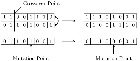
Figure 2.: Single point crossover and bit-flip mutation operator in Genetic Algorithms.
4. Algorithm Families
The main algorithm, at least as was initially introduced, of the seven algorithm families is presented in this section. The motivation for this short introduction is to provide context for our discussion in Section 4.8, Section 5 and Section 8.
4.1. Genetic Algorithms
GAs are a family of stochastic meta-heuristic search algorithms with links to cybernetics (Hol-land 1962, Goldberg and Hol(Hol-land 1988) and philosophically connected to Darwin’s theory of
evolution (Darwin 1858). Social dynamics are simulated based on the premise that the survival
of the fittest paradigm does produce qualitatively better individuals with the passage of several generations. Individuals are in effect decision vectors whose fitness is evaluated using the
objec-tive function. The representation of decision vectors in the basic GA is a binary string termed
chromosome comprised ofgenes (decision variables). Each chromosome is mapped to a
pheno-type. A phenotype is a representation that the objective function can directly utilize to evaluate
the fitness of an individual. The main operators used in GAs are crossover and mutation. These
Algorithm 2 Simple Genetic Algorithm
1: Initialize Population
2: repeat
3: Evaluate Objective Function
4: Apply Crossover and Mutation
5: Select solutions for next population
6: until Termination Condition is Met
two operators are combined in a fashion to balance exploitation and exploration of the search space. Crossover and mutation, see Fig. (2), are applied to the chromosomes thus facilitating the creation of an abstraction layer with respect to the phenotype. This layer of abstraction insulates the internal implementation of GAs from the problem structure, specifically the rep-resentation type of the decision variables. The main operators in GAs have been extended to deal directly with continuous decision variables (Deb and Agrawal 1994, Ono and Kobayashi 1997, Voigt et al. 1995) which is useful when full machine precision is required and all decision variables are continuous.
4.2. Evolution Strategies
inspirational background to GAs, there are two distinct differences. First ES do not employ a crossover operator, and second, ES utilize real decision variables as opposed to GAs that
originally employed binary encoded strings. However, these differences have blurred over time
due to developments on both sides. Effectively both methodologies pursued adaptation and were inspired by the cybernetic movement of that era.
There is a general consensus that both mutation and recombination operators perform an important role and eventually both were employed to various degrees in these two approaches. The main argument concerns their effect on the evolving population. Holland, with his famous building block hypothesis (BBH) (Holland 1975), promoted the idea that the recombination
operator had a positive influence on the evolving population due to short schemas with good
fitness recombining to form even better individuals. Beyer argued that this was not the case; his
suggestion was that the crossover operator had the effect of genetic repair (Beyer 1997). Beyers’
hypothesis was that the features that survive the crossover operator were the ones common to
both parents and not the small schemas with desirable elements.
As previously mentioned the first version of ES was (1 + 1)-ES. This notation refers to the
fact that there are two members in the population, namely the parent and one offspring and
the selection for the surviving individual is performed among the two. The + sign essentially
refers to the selection mechanism. Some later versions of ES use the comma notation, denoting
that theparent takes no part in the selection process and new individuals are selected only from
the offspring pool. The main search operator in (1 + 1)-ES is the mutation operator defined as
follows,
x(G+1)=x(G)+N(0, σ) (6)
were N(0, σ) is a vector of random numbers of size n drawn from the normal distribution with
zero mean and σ standard deviation. Here x(G) represents the parent solution and x(G+1) the
offspring. Iff(x(G+1))≤f(x(G)) the offspring is retained and the parent is discarded. Otherwise the same parent is used in the next generation.
ES were extended to a true population-based optimization methodology by Schwefel (1981).
Schwefel introduced (µ+λ)-ES as well as (µ, λ)-ES. Here µis the number of parents producing
λ offspring. The resulting population, after the selection process, is reduced to the number of
parents µ. Schwefel combined these two variants to enable a parallel implementation of ES as
well as to experiment with adaptation in the control parameters such as σ (B¨ack et al. 1991).
For further details on the (µ+λ)-ES the reader is referred to (Schwefel 1981, B¨ack et al. 1991,
Beyer and Schwefel 2002).
4.3. Artificial Immune Systems
The immune system (IS) is a fine tuned concert of a vast array of cells acting in synchronism in order to protect the body from pathogens. Pathogens are substances or microorganisms that can
affect the balance of the body (homeostasis), impairing its normal functioning and even cause
death. The immune system responds,immune response, to such threats creating specialized cells
capable of neutralizing pathogens and restoring balance. In order for this procedure to progress smoothly the immune system must attack the source of the disturbance while minimizing the
effect this action has on healthy cells in the body -specificity. Once a particular threat has been
dealt with, the second time the body is exposed to the same pathogen the immune response will be swifter and stronger to such a degree that the organism might not even realize that it had
been afflicted by a pathogen, so the immune system also exhibits memory.
Pathogens have certain features that the immune system can identify. These features are
called antigens, and their presence in the organism is detected by antibodies. Antibodies are
Variable Part Epitope Antigen
[image:9.595.227.403.125.250.2]Antigen
Figure 3.: Antibody schematic diagram.
see Fig. (3), identifies an antigen by binding on it, thus serving as a beacon signalling other cells in the immune system to devour the intruder. Although antibodies are highly specialized, their diversity is enormous thus enabling the immune system to attack a vast variety of antigens. When a particular antigen is identified the antibody that successfully identified it will proliferate
by cloning via a process termedthe clonal selection principle (Mohler et al. 1980, Dasgupta and
Forrest 1999). Once the pathogens have been eliminated, superfluous antigens are dissolved
mainly via the process of apoptosis (Krammer 2000). However some cells responsible for the
proliferation of this particular type of antibodies survive as memory cells (Parijs and Abbas 1998), and if the host is infected again by the same pathogen these memory cells will be activated
to produce antibodies much faster compared with the first encounter, primary response, with
this particular antigen.
Although this introduction to the immune system will serve the purpose of illustrating the parallelism of the biological system with Artificial Immune Systems (AIS), it does not even scratch the surface of the delicate intricacies present in the immune system. The interested reader is referred to (Parham and Janeway 2005).
AIS have been employed in various applications, such as intrusion detections systems, virus detection, anomaly detection fault diagnosis, and pattern recognition (Dasgupta and Attoh-Okine 1997). AIS have been used in place of fitness sharing techniques in GAs to maintain diversity and distribute the population evenly along the PF (Coello and Cort´es 2005). Another
interesting use is in time dependent optimization problems where AIS successfully adapt to
a changing problem (Gasper and Collard 1999). Despite these applications, direct use of AIS to optimization problems prior to 1999 is scarce. This could potentially be attributed to the complexity involved in implementing an AIS.
Figure 4.: Similarity measure used to simulate the clonal selection principle (Coello and Cort´es
2002). Here, x,yrepresent an antigen and antibody respectively. The similarity measure, f(·,·),
[image:9.595.240.381.617.732.2]Although there is no single uniform framework that describes AIS for optimization, a represen-tative algorithm based on the principles of immune systems is due to Coello and Cort´es (2002). Here we describe the main features of this method, while for further details the reader is referred to Coello and Cort´es (2002, 2005). Coello and Cort´es (2002) draw upon the the clonal selection principle by labelling elite individuals as antigens; these are solutions that are non-dominated
and feasible. Inferior individuals where labeled as antibodies, namely solutions that are either
infeasible, dominated or both. Subsequently a modified Hamming distance metric was employed for fitness assignment,
f(x,y) =dH(x,y) +m, (7)
where m is an additional biasing factor that depends on the number of similar groups found
between, x and y. An illustration of the calculations involved in evaluating (7) as well as a
definition of m is given in Fig. (4). Subsequently the mutation strength for the generation of
new individuals is determined by a reverse proportional relationship with (7) (Coello and Cort´es 2002). The aforementioned algorithm cannot be classified as a modified genetic algorithm as new individuals are formed only by means of mutation. In this respect the method presented by Coello and Cort´es (2002) is similar to ES.
4.4. Ant Colony Optimization
Ants come from the same family as wasps and bees Choe and Perlman (1997), namely
Hy-menoptera Fromicidae. As individuals, ants’ capabilities are limited. Apart from their extraor-dinary strength their sight is very limited and their hearing and sense of smell depend on their antennas. Despite these facts, ants as a collective exhibit very interesting behaviour patterns (Deneubourg et al. 1990). In their search for food, ants explore their nest surroundings in a random-walk pattern. However, when an ant discovers food, it returns to the nest releasing pheromones (Deneubourg et al. 1990) of varying intensity depending on the quality and quan-tity of the discovered food source. Other ants close to the pheromone trail are more likely to follow that path and, if there is still food to be found at the end of the trail, they release pheromones as well, thus reinforcing the pheromone scent which in turn increases the proba-bility that more ants will follow that path. Alternatively when an ant reaches the destination indicated by the pheromone trail and does not discover anything interesting, no pheromone is released and progressively the path becomes less and less attractive as pheromones evaporate.
Dorigo et al. (1991) introduced an algorithm, Ant System (AS), inspired by the emergent
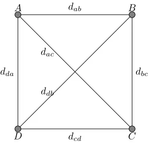
behaviour of ants. The AS was tailored to solve combinatorial problems and the travelling salesman problem (TSP) was used as a test bed, see Fig. (5). Almost a decade later Dorigo and Di Caro (1999) formalized the AS and other similar methods in a unified framework, ant colony
optimization (ACO). ACO is comprised of N individuals called ants. These are distributed
amongµcities and each ant progressively creates a candidate solution for the problem. The ants
decide which city they will next visit based on the pheromone trail (τ) associated with each edge leading to a particular city and the separating distance of the cities. Assuming that an ant
starts off from cityA in Fig. (5), it has three options, namely to go toB,C orD. Each of these
edges has a pheromone trail associated with it. The probabilistic transition rules are controlled
by two parameters, namelyτ andη. The parameterτ can be initialized using prior information,
if available, or with the same value for all edges. Initiallyη represented thevisibility of the ants
which depended on the distance of a city from the next and was defined as, ηAB = dAB1 for the
edge connecting city AwithB. The smallerηAB is, thus the larger the distancedAB is, the less
likely is that an ant in city A to choose the city B for its next step in the tour, see (9). As
A B
C D
dab
dbc
dcd
dda
dac
[image:11.595.236.384.130.272.2]ddb
Figure 5.: Travelling salesman problem with four cities. Although the edges connecting the cities
seem equidistant they need not be. The distance of two cities is represented by d.
updated as,
τi,j= (1−ρ)τij + N
X
s=1
∆τi,js (8)
where ρ is defined as the evaporation rate of the pheromones, and ∆τi,js is the amount of
pheromone added by ant s on the edge connecting the ith and jth node. Therefore, the larger
the deposit of pheromones across an edge i, j the larger τi,j is, hence the probability that more
ants will select this path is increased. The probabilistic transition rule, based on τ and η, that
govern the behaviour of ants is summarised by the following relation,
pi,j =
τα i,jη
β i,j µ P m=1
τα i,mη
β i,m
if j is a valid destination
0 if j is not a valid destination,
(9)
where a valid destination for an ant is a node that the particular ant is allowed to visit at that
particular stage. The probability that an ant on node iwill visit a node j is given by pi,j, and
µ is the number of nodes in the problem. For the TSP problem a node is a valid destination
if a particular ant has not visited that node. Also α and β are real and positive numbers used
to favour either τ or η; ifα=β the information gained from τ is considered equally important
with η.
The general ACO algorithm has the following stages,
Step 1 Initialize pheromone values τ for all the edges. Usually all the edges receive the same pheromone value at the start of the algorithm unless prior information is available indi-cating that favouring certain edges would increase convergence speed.
Step 2 Construct a solution for each ant,xs.
Step 3 Update the pheromone values for each edge.
Step 4 Go to Step 2 until stopping criteria are met.
The rules for constructing a solution xs for each ant are problem-dependent.
+ Minimum
+ dv2
dv1 x(rG2) x
(G) r3
F(x(rG2)−x
(G)
r3 )
x(rG1)
[image:12.595.209.422.117.323.2]v(iG+1)
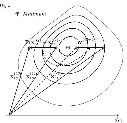
Figure 6.: Illustration of the mutation operator in DE, in this case F = 1 and x(iG+1) =v(iG+1)
since for this instance f(x(iG+1))< f(x(iG)), and,dv1 anddv2 stand for decision variable one and
two respectively.
4.5. Differential Evolution
DE was introduced by Storn and Price (1995) as a global search method over real decision vectors, although later extended versions for integer (Lampinen and Zelinka 1999) and binary representations (Pampara et al. 2006) were introduced. The major strengths of DE are its con-ceptual simplicity, ease of use and implementation; also the number of tuning parameters is very small and the same parameter values with no or very little change are found to be applicable to a wide range of problems.
For a population of size N and decision vectors of dimensionn, the current generation is
x(iG) fori={1,2, . . . , N}. (10)
The basic DE algorithm has three stages in its iteration phase: mutation, crossover and selection. During the mutation stage all decision vectors in the population are perturbed resulting in a
temporary new population V(G+1) of the same size with X(G). The mutation operator in DE is
described as,
∀x(iG),i={1,2, . . . , N},
v(iG+1) =x(rG1)+F
x(rG2)−x
(G)
r3
,
(11)
and if f(vi(G+1)) < f(xi(G)) the newly formed parameter vector v(iG+1) is assigned to x(iG+1), otherwise x(iG) is retained in the next generation. The parameters r1, r2, r3 ∈ {1,2, . . . , N} are
sampled at random without replacement from the set{1, . . . , N} − {i}for each individual in the
population. The parameter F ∈[0,2] is a scaling factor controlling the variation (x(rG2)−x
(G)
+ Minimum
+ dv2
dv1 pi
x(iG) pg
M
[image:13.595.208.424.118.321.2]v(iG) x(iG+1)
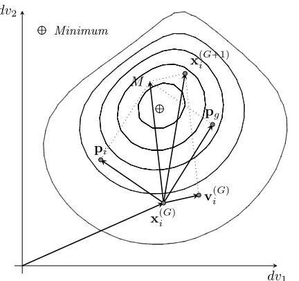
Figure 7.: Particle update illustration in particle swarm optimization. Where,M =c1U(0,1)(pi−
x(iG)) +c2U(0,1)(pg−xi(G)) andc1U(0,1), c2U(0,1) = 1 for clarity. As before,dv1 anddv2 stand
for decision variables 1 and 2 respectively.
The crossover operator in DE is defined as
u(iG+1)=u(i,G1+1), u(i,G2+1), . . . , u(i,nG+1),
where
u(i,jG+1)=
(
v(i,jG+1) U(0,1)≤Cr or j =ridx(i), x(i,jG) U(0,1)> Cr and j6=ridx(i),
j = 1,2, . . . , n ,
(12)
and Cr is the crossover rate parameter, bounded in the range [0,1], ridx(i) is a random index
in the range {1, . . . , n},1 and U(0,1) is a random number sampled from a uniform distribution
in the domain [0,1]. Once the new decision vectorsu(iG+1) have been generated, the selection is
based on the greedy criterion, which can be stated as
x(iG+1)=
(
ui(G+1) if f(ui(G+1))< f(x(iG))
x(iG) otherwise. (13)
So the DE algorithm progresses exactly asAlg. 2but using the crossover, mutation and selection
operators defined above, in place of the variation operator. Some general guidelines on tuning DE can be found in (Storn 1996).
4.6. Particle Swarm Optimization
Particle swarm optimization, introduced in (Eberhart and Kennedy 1995, Kennedy and Eberhart 1995) was inspired by the flocking behaviour of birds and swarm theory. In PSO, as observed in nature, each agent has a rather limited repertoire of behaviours while the collective exhibits
complex expressions. In the initial PSO algorithm the particles (decision vectors) use a simple update rule to update the velocity and, consecutively, the position of each particle. An archive is maintained that contains the best achieved objective function values for each particle
P={p1,p2, . . . ,pN}, (14)
so f(pi)≤f(x(iG)) and if f(pi)> f(x(iG+1)), thenpi=x(iG+1) and so on. Additionally a global
best position is maintained pg for which the following condition must hold f(pg)≤f(x(iG+1)),
for all i ∈ {1,2, . . . , N}. If this is not true pg is updated using the following rule pg = {xi :
min
i f(xi)}. The velocity update rule is:
vi(G+1)=vi(G)+c1U(0,1)
pi−x(iG)
+c2U(0,1)
pg−x(iG)
,
(15)
where c1 and c2 are positive constants and U(0,1) is a random number in the range [0,1]. A
suggested value for c1 and c2, for problems when no prior information is available, is that both
are set to 2 (Kennedy and Eberhart 1995). This would effectively result in a multiplier with a
mean value of one, thus balancing in the mean the bias toward the point pg and pi for each
particle (Shi and Eberhart 1998). A modification to (15) was presented by Shi and Eberhart
(1998) introducing a multiplying factor w to v(iG), the inertia weight, resulting in the following
velocity update relation,
vi(G+1)=w·vi(G)+c1U(0,1)
pi−x( G)
i
+c2U(0,1)
pg−x(iG)
,
(16)
where w can be constant, a function of the current generationG or even a function of a metric
measuring the convergence of the algorithm. (For example the normalized hypervolume indicator
could be utilized.) A value of 1 for w results in the regular velocity update rule, while a value
below 1 progressively decreases the average velocity of the particles biasing the search to regions local to the particles. Alternatively, a value above 1 leads to a progressive increase in the velocity of particles resulting in a more explorative behaviour. Subsequently the position of the new particles is calculated in the following way,
xi(G+1) =xi(G)+vi(G+1) . (17)
PSO does not have an explicit selection operator, although the archive p could qualify as such.
Several variants of the described PSO algorithm have been devised, the interested reader is referred to (del Valle et al. 2008, Tripathi et al. 2007). Other interesting methods that cannot be classified as particle swarm optimizers but inherit some features are the group search algorithm (He et al. 2009) and several variants of the bee colony optimization (Akay and Karaboga 2012, Karaboga et al. 2012,?).
4.7. Estimation of Distribution Algorithms
crossovers (Ono and Kobayashi 1997) and fuzzy recombination (Voigt et al. 1995), to name but a few. These crossover operators, although they did not recombine more than two or three individuals from the population, did use a probability distribution that was based on the parent solutions to generate the offspring. Estimation of distribution algorithms can, in a way, be seen as an expansion to the idea behind these crossover operators. The generalization is straightforward. Instead of using a crossover and mutation operator in the GA, a probability distribution over the most prominent of solutions can be estimated and then utilized to produce new individuals
in the population (M¨uhlenbein and Paass 1996). Arguably, another source of inspiration in the
creation of EDAs has come from the statistics community, for example, the cross entropy method (Rubinstein 1999, 2005) was initially used for rare event estimation and probability collectives (Bieniawski et al. 2004) has a game theoretic foundation (Bieniawski 2005, Wolpert et al. 2006).
A typical EDA, see Alg. 3, proceeds very similarly to a GA. The difference is that on every
generation a subset of the population, usually the better half of the population, is selected and
based on that subset a probabilistic model is created. Then this model is sampled and the resulting new individuals are merged with the old population while maintaining the population size constant.
Algorithm 3 Estimation of Distribution Algorithm
1: Initialize population X(0)
2: Evaluate objective function
3: repeat
4: Select promising solutionsXp from X(G)
5: Create a probabilistic model P based onXp
6: Generate new solutionsXn by sampling P
7: Evaluate the objective function for Xn
8: Combine Xn and X(G) to createX(G+1)
9: until Termination condition is met
While EDAs have successfully been applied to a diverse problem set, involving real and discrete decision variables, outperforming rival algorithms (Hauschild and Pelikan 2011), it is not so trivial to generate the required probabilistic model. Also, the model type strongly depends on the decision variable type, whether or not the decision variables are coupled, to what extent and in what way. Assuming that all decision variables are independent, while in fact there are multiple interdependencies would grossly mislead the algorithm (Pelikan et al. 2002). Additionally these challenges increase in difficulty when dealing with MOPs (Laumanns and Ocenasek 2002, Sastry et al. 2005). Despite these difficulties, further research in EDAs seems promising due to their inherent adaptive nature that enables them to scale well compared with other algorithms for some problems (Shah and Reed 2011). Another strong point is that prior knowledge can effectively be exploited by biasing directly the initial population (Sastry 2001) or by biasing the model creation procedure (Muhlenbein and Mahnig 2002). However as seen in Fig. (14) the research activity in EDAs is still in relatively low levels, a fact that can be ascribed to the difficulty of creating a probabilistic model capable of capturing dependencies in a way that doesn’t substitute one difficult problem, namely the original optimization problem, with another, that of building a probabilistic model.
4.8. So Why Not a Single Approach?
As is seen in Fig. (14), the number of publications appearing per year is constantly increasing for all the above algorithm families, albeit not at the same pace. However given their similarities
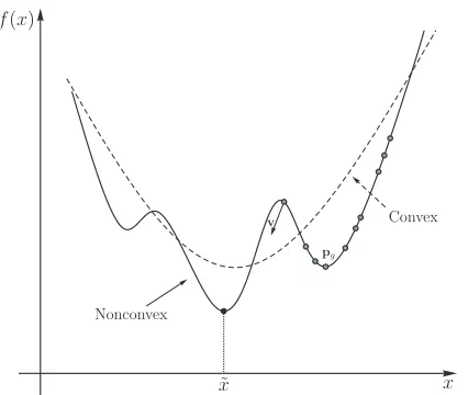
Figure 8.: Illustration of a convex (dashed line) and nonconvex (continuous line) multi-modal
function. The points on the nonconvex function represent a swarm of solutions in a PSO
algo-rithm.
away. This seems not to be the case for the above seven algorithm families, which is one of the reasons we elected to present them in this work.
Thissurvival must mean that there is a niche that every family fulfills better than the others,
while no algorithm family is dominated1 by any other in terms of performance. This result is
not surprising and is partially explained in (Wolpert and Macready 1997). However, that niche seems to be rarely expressed, with a few exceptions of course, for example ACO are renown for their applications on combinatorial problems, see Fig. (15), but what of the others? At this point we exploit what (Ullman 2009) considers to be a bad practice in research, namely for researchers to explore the unsolved problems reading the conclusions of published articles and focusing their work on the problems that they can solve. If this is in fact what is common practice, which (Michalewicz 2012) seems to agree with, then we will be able, to some extent, to identify the strengths and weaknesses of the aforementioned algorithm families by the number of papers published with respect to different problems, see Fig. (15).
Consider convex optimization algorithms. In this class gradient information is exploited to determine a direction of search. However real-world problems do not always conform to the structure that such a class of optimization methods can attack. One way that a problem can fail the convexity test is illustrated in Fig. (8). This type of problems are called multi-modal and have multiple local optimal. In this setting a particle swarm optimization algorithm would very well suited as it is conceivable that in the depicted scenario in Fig. (8) a PSO based algorithm
has the potential to overcome the ridges and locate eventually the global optimum, ˜x. However
the fact that the swarm of solutions in Fig. (8) has reached to that location is due to their
following the solution pg which in turn follows a path that is similar to that of a gradient
descent algorithm. For this problem an algorithm with more aggressive stochastic operators
would require more function evaluations compared to PSO. Problems with this structure are prevalent in evolutionary algorithm test functions, for example see (Deb et al. 2002, Huband et al. 2006, Saxena et al. 2011). For the same reasons differential evolution would have the potential to perform well in such a class of problems.
Now consider a different type of nonconvex function, see Fig. (9). In this case theridge would
be more difficult to cross using PSO, however it would be much easier for an algorithm whose
stochatic component is more dominant, for example ES or EDAs. Of course given the number
Figure 9.: A discontinuous objective function. The minimum is located in the left lobe however
algorithms with weak stochastic components that most of their initial population is located in
the right lobe will have difficulties in locating the global optimum.
of cross-over operators available for GAs it could be argued that such a behaviour could be simulated by judicious selection of such operators. Moreover we neglected the fact that all the
aforementioned methods have tunable parameters, which in turn alter their behaviour.
Never-theless, the different conceptual paradigms may enable the practitioner select these parameters more easily for a certain type of algorithms when applied to a problem with a structure that
favours that particular algorithm family.
5. Multi-Objective Problems
When the objective function is vector valued, that isF: Rn→Rkthen the optimization problem
becomes more complex. This complexity stems from the fact that now there exists the possibility
that there is no single objective function value F(˜x)≤F(x) for allx∈Rn, as was the case for
single objective problems. Therefore, in all but the most trivial case where all the scalar objective
functions are harmonious, namely when all the objectives are positively correlated (Purshouse
and Fleming 2003), only a partial ordering can be induced without the preference structure of the decision maker.
5.1. Problem Setting
A multi-objective minimization problem can be defined as follows:
min
x F(x) = (f1(x), f2(x), . . . , fk(x))
subject tox∈S,
(18)
where k is the number of objective functions, S, is the feasible set in decision space, x is the
decision vector and, fi(x), are scalar objective functions. Let F: S → Z, namely the forward
image of the objective function, then the set, Z, is the feasible set in objective space. The
min
x F(x) notation is interpreted as: minimise the vector valued function F(x) over all x ∈ S
Figure 10.: Pareto optimal set and weakly Pareto optimal set. Note that the Pareto optimal set is a subset of the weakly Pareto optimal set.
unconstrained minimization problem depending on howSis defined, see (5). Further the fact that
minimization is assumed is not restrictive because the problem of maximising −f is equivalent
to the problem of minimising f and vice versa. In the special case wherek= 1, (18) becomes a
single objective minimization problem. It is implicitly assumed that the scalar objective functions are mutually competing and perhaps are incommensurable while the goal is to minimise all of them simultaneously. If this is not the case then no special treatment is needed since minimising one of the scalar objective functions automatically results in minimization of the rest.
5.2. Definitions
The problem that arises in MOPs is that direct comparison of two objective vectors is not as
straightforward as in single objective problems. In single objective problems when bothx,x˜∈S
and f(˜x)< f(x) it is clear1 that the decision vector ˜xis superior tox. This is not the case when
two or more objectives are considered simultaneously and there exists no a priori preference
toward a particular objective.
If the relative importance of the objectives is unspecified, one way to partially order the
objective vectors, z ∈ Z, is to use the Pareto2 dominance relations, initially introduced by
Edgeworth (1881) and further studied by Pareto (1896). Specifically, in a minimization context,
a decision vector ˜x∈S is said to bePareto optimal if there is no other decision vector x∈S
such that fi(x)≤fi(˜x), for all i, and, fi(x)< fi(˜x) for at least onei= 1, . . . , k. Namely there
exists no other decision vector that maps to a clearly superior objective vector. Similarly, a
decision vector ˜x∈S is said to be weakly Pareto optimalif there is no other decision vector
x ∈S such that fi(x)< fi(˜x) for all i= 1, . . . , k, see Fig. (10). Furthermore, a decision vector
˜
x ∈ S is said to Pareto-dominate a decision vector x iff fi(˜x) ≤ fi(x), ∀i ∈ {1,2, . . . , k}
and fi(˜x) < fi(x), for at least onei ∈ {1,2, . . . , k} then ˜x x. So, in terms of generalised
inequalities, if F(˜x)F(x) andF(˜x)6=F(x), then ˜xx. Also, a decision vector ˜x∈S is said tostrictly dominate, in the Pareto sense, a decision vectorxifffi(˜x)< fi(x), ∀i∈ {1,2, . . . , k}
then ˜x ≺x. That is, if F(˜x) ≺F(x), then ˜x ≺x. It should be noted at this point, that when
≺, are used in decision space, their meaning is mostly symbolic and is used to reflect the
dominance relations in the objective space. The Pareto dominance relations with respect to a
1For a minimization problem.
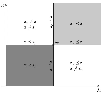
Figure 11.: Pareto dominance relations in the objective space. The dark gray region contains
clearly better solutions compared with zp, the light gray region clearly worse solutions, while,
the two other regions contain solutions incomparable to zp.
solution in objective space, zp, are depicted in Fig. (11).
Most multi-objective problem solvers attempt to identify a set of Pareto optimal solutions, this
set is a subset of the Pareto optimal set(PS) which is also referred to as Pareto front(PF).
The Pareto optimal set is defined as follows:P ={z:∄˜zz,∀˜z∈Z}. The decision vectors that
correspond to the set,P, are also called the Pareto set and are denoted asD, namelyF:D → P.
The most widely used measures of the quality of the obtained Pareto front are the generational
distance (GD), its inverted version (IGD) (Van Veldhuizen 1999) and the hypervolume indicator (Zitzler and Thiele 1999). A detailed discussion of these and other metrics is beyond the scope of this work, however there is a number of excellent works that address this issue, for example Zitzler et al. (2003), Zhou et al. (2011).
6. Methods for Extending PBOTs to MOPs
In what follows the main methodologies used to extend population-based optimization techniques to address multi-objective problems are discussed. These are separated into 3 broad categories, namely:
• Pareto-Based Methods
Pareto-based methods employ Pareto-dominance relations to evaluate the quality of the population. These methods are still used to this day, however it would appear that their ability to handle problems with more than 3 objectives (many-objective problems) is some-what limited (Ishibuchi et al. 2008).
• Decomposition-Based Methods
Decomposition methods employ a scalarizing function and a set of weighting vectors to
• Indicator-Based Methods
This type of methods for multi-objective problems is also promising, for example see
(Wang et al. 2012), and are based on metrics developed to measure the quality of the
solution set obtained from a PBOT. The most prevalent of these indicators has been the hypervolume indicator which was introduced in the context of multi-objective optimization by Zitzler and Thiele (1999).
Schaffer (1985) was the first to extend GAs to become multi-objective problem solvers. In retrospect, his approach may appear simple, but for its time it was quite a conceptual leap since
VEGA considered all objectives simultaneously. VEGA, see Alg. 4, partitioned the population
x into k equally sized randomly selected sub-populations, wherek is the number of objectives.
Then each partition is assigned to an objective and individuals are ranked according to their performance for the corresponding objective and a mating pool is formed using proportionate selection as described in (Goldberg 1989). Crossover and mutation operate on the entire
popula-Algorithm 4 VEGA
1: X(1)←Initialize 2: G←1
3: ps←N/k ⊲ Partition size
4: repeat
5: X(G)←Shufflerows(X(G))
6: fori←1, kdo ⊲ Partition the population
7: Di ←Xps(G×)(i−1)+1→i×ps
8: Ei←Evaluate(Di)
9: Si←Proportionate Selection(Ei, Di)
10: end for
11: X˜(G)←Join(S1,...,k)
12: X˜(G)←Crossover(X˜(G)) 13: X(G+1)←Mutate(X˜(G))
14: G←G+ 1
15: until G≤M axGenerations
tion in the hope that linear combinations of the fitness functions would arise thus estimating the
entire PF. This however was to some extent problematic since a phenomenon called speciation
(Schaffer 1985) did on some occasions occur. For instance in objective functions with a concave PF, VEGA fails to approximate the PF as parts of the population drift toward the edges favour-ing one of the objective functions. Other methods employfavour-ing the same or very similar approach are due to Fourman (1985) and Kursawe (1991), a variant applied to evolution strategies. A more recent work investigating VEGA is due to (Toroslu and Arslanoglu 2007).
6.1. Pareto-Based Methods
Fonseca and Fleming (1993) were the first to use Pareto dominance relations in a multiple objective genetic algorithm (MOGA), while incorporating progressive preference articulation enabling the decision maker to guide the search interactively. The dominance relation was used to rank the individuals in a population in a way similar to a set of selection methods proposed by Fourman (1985). Every individual in the population, after evaluation of the objective function, is ranked using the following relation,
Figure 12.: Ranking method used in MOGA. The numbers above the points represent the rank
of the individual that results in that objective vector. The worst rank possible is N.
where pi is the number of individuals dominating the decision vector xi. The idea behind this
method of ranking, see Fig. (12), is that misrepresented sections of the PF will increase the selection pressure to that direction of the front. As an example, the objective vector with rank 3 as seen in Fig. (12) is dominated by two individuals while the objective vector with rank 2 is
dominated only by one. Alternatively, this means that within area Athere is only one solution,
while in area B there are two suggesting higher concentration of solutions. This information
is used to induce better spread in the objective vectors that are not part of the current PF
approximation so as to maintain a relatively even supply of objective vectors in all regions of
the PF. For the objective vectors that are part of the PF approximation, Fonseca and Fleming
introduced an adaptive factor,σshareto penalize objective vectors that are less thanσshareapart.
Lastly a facility for progressive preference articulation was embedded in MOGA providing the
means for the DM to narrow down the search to interesting regions of the PF (Fonseca and
Fleming 1993, 1995). This facility is implemented by incorporating a goal attainment method in the ranking procedure. Let g ={g1, . . . , gk} be the goal vector and z1 ={z1, . . . , zk} and z2
be two objective vectors. A preference relation can be expressed such that whenk−s of thek
objectives are met then z1 ispreferable to z2 if and only if,
z(1,1...k−s)z(2,1...k−s) or
{(z(1,1...k−s)=z(2,1...k−s))∧
[(z(1,k−s+1...k)z(2,1...k−s+1...k))∨
(z(2,k−s+1...k)6≤g(k−s+1...k))]} (20)
The rest of the MOGA utilized Gray encoding for the chromosomes, two point reduced surrogate crossover and the standard binary mutation.
Another prominent algorithm, the non-dominated sorting GA (NSGA), that utilized the Pareto dominance relations was proposed by Srinivas and Deb (1994). This method is almost identical to the non-dominated sorting idea proposed by Goldberg (1989). Non-dominated sorting is very similar to a well established concept in non-cooperative game theory in which candidates need to
select a winning strategy while considering what their opponents’ strategy might be. This idea
is usually referred to as eliminating dominated strategies which is an iterative process of deleting
Figure 13.: Non-dominated sorting method as used in NSGA.
thus result in unfavourable outcomes. Interested readers are referred to (Bernheim 1984). Non-dominated sorting, see Fig. (13), works as follows:
Step 1 Evaluate the objective function for each individual in the populationX.
Step 2 Find the non-dominated individuals in the population, Xnd, and remove them from the
current population Xnew={x:x∈(X∩Xnd)c}.
Step 3 RepeatStep 2until no solutions remain in Xnew.
Each non-dominated set identified by this process is labelled as afrontand given a rank according
to the position it has in the iteration. For example, the first identifiedfront would befront 1, the
second front 2 and so on. Subsequently the individuals of each front are assigned fitness values
using the following procedure starting from the first front,
Step 1 Assign to all the individuals in front 1 a fitness value N, where N is the number of individuals in the population.
Step 2 Use sharing to penalize clustered solutions in the current front.
Step 3 Assign the lowest fitness minus a small valueǫto all individuals in the next front and go to Step 2 until all individuals in all fronts have been assigned a fitness value.
The sharing distanceσshare is calculated based on distance in the decision variable space rather
than the objective space and is held fixed throughout the algorithm execution. Finally NSGA employed the roulette-wheel selection operator (Goldberg 1989) and the usual bitwise mutation operator, see Fig. (2). The fact that NSGA uses sharing based on the distance of the decision vectors, seems counter intuitive since equally spaced decision vectors do not necessarily map to equally spaced objective vectors unless the mapping is affine which is usually not the case for most objective functions. This can potentially mislead the algorithm as to which solutions are densely clustered and which are not, resulting in exactly the opposite effect. Although, as the authors state, sharing can be performed based on the objective vectors (Srinivas and Deb 1994),
they do not mention how σshare would be selected in that case. Non-dominated sorting is the
basis of an improved version of NSGA, namely NSGA-II (Deb et al. 2002), which is actively used for benchmaring and improved upon to this day, see (Zhang and Li 2007, Li and Zhang 2009, Ben Said et al. 2010, Wang et al. 2012, Bui et al. 2012).
One problem identified for Pareto-based methods for multi-objective problems, was that good solutions could be lost if they were not retained using some mechanism and the cost to rediscover them can potentially be prohibitive. This situation is exacerbated when the cost, computational or otherwise, of evaluating the objective function is high; this is often the case in most real-world
of highly performing individuals in the population. Zitzler and Thiele (1999) introduced an algorithm named the strength pareto evolutionary algorithm (SPEA) that used elitism. Their approach was not the first to utilize an external archive to retain good performing individuals, however it was certainly one of the earliest and most elegant attempts.
SPEA, in addition to the current population X, maintains an archive population X˜ of
max-imum size ˜N which is usually smaller than the population size N. Zitzler and Thiele (1999)
suggest ˜N = 0.25N. At the start of the algorithm the external archive is empty and the
popula-tion is initialized randomly within the decision variable limits or as appropriate to the problem. After the objective function has been evaluated the population is searched for non-dominated
solutions which are copied to the archive X˜ = Xnd. This direct assignment is performed only
on the first iteration of the algorithm. In subsequent iterations the archive updating procedure
is different if the total population in the archive exceeds ˜N. When the archive size becomes
larger than ˜N, the superfluous solutions are removed based on a crowding algorithm that the
authors of SPEA introduced. This crowding algorithm maintains the elite solutions that have
maximal spread along the PF. After the archive size is properly reduced to its maximum size,
the population and the elite individuals are assigned fitness values in the following way:
Step 1 Assign fitness values, called strength (s), to the population in the archive X˜, using the
following relation, si = Nn+1i , where ni is the number of individuals that the ith solution
in the archive dominates in the regular population X.
Step 2 The regular population X is then assigned fitness values according to, fi = 1 + P xjxi
si.
Note that in SPEA lower fitness value is considered to be better. Therefore, if a decision
vector xi is not dominated by any individual in the populationX, its fitness, fi, would be
equal to 1.
The way the archive is maintained and used in SPEA ensures that the populationXis rewarded
when it approaches the PF. In a way the archive is used as amoving target to which the regular
population aspires. Again the rest of the algorithm utilizes roulette wheel selection and random bit mutation.
6.2. Decomposition-Based Methods
As mentioned in Section 6, decomposition methods depend on scalarizing functions to break down a multi-objective problem into a set a single objective subproblems. The premise of this approach is that, the methods described in Section 4, can be applied almost unaltered. This benefit however, takes its toll as the selection of the weighting vectors controls the distribution of solutions on the Pareto front (Giagkiozis et al. 2012, 2013). This issue has been investigated in some detail in (Giagkiozis et al. 2013), where it is shown that the algorithm scalability to many-objective problems can be significantly affected if an arbitrary method is employed in the selection of the weighting vectors.
A family of scalarizing functions is the weighted metrics method (Miettinen and M¨akel¨a 2002):
min
x k
X
i=1
wi|fi(x)−zi⋆|p
!
1
p
, (21)
where w= (w1, . . . , wk) is referred to as weighting vector andwi are the weighting coefficients.
The weighting coefficients can be viewed as factors of relative importance of the scalar objective
functions in F(·). The weighting coefficients must bewi ≥0 and Pik=1wi = 1, also p ∈[1,∞).
However p is usually an integer or equal to∞. A potential drawback of weighted metrics based
can be estimated adaptively during the process of optimization (Zhang and Li 2007). When
p=∞the Chebyshev scalarizing function is obtained:
min
x kw◦ |F(x)−z ⋆| k
∞. (22)
The ◦ operator denotes the Hadamard product which is element-wise multiplication of vectors
or matrices of the same size. The key result that makes (22) very interesting is that for every Pareto optimal solution there exists a weighting vector with coefficientswi >0,for alli= 1, . . . , k
(Miettinen 1999). Meaning that all Pareto optimal solutions can be obtained using (22). This result is quite promising, although in current practice the choice of weighting vectors is made
primarily using ad hoc methods, see (Das and Dennis 1996, Jaszkiewicz 2002, Zhang and Li
2007), and so the points on the Pareto front cannot be controlled effectively.
The immune system based algorithm proposed by Yoo and Hajela (1999) used the weighting
method (Miettinen 1999, pp. 27), which is obtained by setting p = 1 and z⋆ = 0 in (21). The
weighting method aggregates all the objective functions into a single function using the following relation,
min
x g(x) = k
X
i=1
wifi(x)
k
X
i=1
wi = 1, and,wi ≥0, for all i
subject tox∈S,
(23)
wherewi represents weight of the ith objective function. When all of the objective functions are
equal in importance to the decision maker, the weights can be set to wi = k1, where k is the
number of objective functions. Using the weighting method results in an approximate solution for one point of the PF. To explore more points, various combinations of the weights have to be used. Yoo and Hajela (1999) randomly generated a set of weight combinations in an attempt to uniformly sample the PF, and then used these different weighting vectors to guide the search.
Some difficulties encountered in the above implementation are that the weighting method is used and its weaknesses could affect the algorithm in several ways. For instance, evenly spaced weighting vectors do not necessarily produce an even distribution of points along the PF and two widely differing weight vectors need not produce significantly different points along the PF (Miettinen 1999). An additional shortcoming of the weighting method is that it cannot guarantee that all the Pareto optimal points can be obtained (Miettinen 1999, pp. 80). It is apparent, even
in this early application of AIS to MOPs that there is a jump in algorithm complexity when
compared to a GA. This complexity inevitably leads to an increased demand on computational resources. This cost will have to be justified especially since GAs, as can be seen in (Fonseca and Fleming 1993), can explicitly deal with constraints as well. However, the computational cost of most algorithms can often be ignored when compared with the cost of evaluating the objective function. Nevertheless this increase in algorithm complexity is not due to the use of the weighting method.
concave PF is unstable and attracts solutions toward the two extremes1 for which the weights
are (0,1) and (1,0) respectively, this view is further supported in (Giagkiozis and Fleming 2012).
However, in real world applications, the PF shape is usually not known a priori. To deal with
this predicament Jin et al. (2001) suggested that if the optimiser is run with weights of one
of the two extremities of the PF, that is either (0,1) or (1,0) and then gradually or abruptly
the weighting vectors are exchanged the optimiser should be able to traverse the entire PF. To capture the Pareto optimal solutions Jin et al. suggested an archiving technique that would, hopefully, result in a good approximation of the entire PF. The problem with this technique is that the optimiser is effectively segmented in two phases, the first one with the fixed weighting
vectors and the second one where the population is allowed toslide along the PF. To successfully
accomplish this task, a metric is needed to measure the convergence rate of the first phase so that the second phase is initiated. This task is not trivial because it presupposes that the minimum is already known. Another potential problem is that if disjoint regions in the decision variable space map to neighbouring objective values, this approach will have difficulty approximating the PF. Lastly, it is difficult to envisage how would this method scale to problems with more than 2 objectives. Despite these difficulties, the aforementioned approach seems to perform reasonably well for the test problems used in (Parsopoulos and Vrahatis 2002, Jin et al. 2001).
As mentioned in Section 3, the main algorithm in PBOTs is usually built with single objective optimization in mind and as such the extension to multiple-objectives, as it will be apparent by now, requires a number of considerations. For instance, diversity preserving operations and
eliteness preserving strategies inevitably result in higher computational costs. And for algo-rithms utilizing directly the non-dominated sorting strategy (see Section 6.1), the cost is even higher. Relatively recently a multi-objective evolutionary algorithm based on decomposition (MOEA/D) was introduced by Zhang and Li (2007) as an alternative way of extending DE and evolutionary algorithms (EAs), in general, to deal with MOPs. The approach depends on one of several available decomposition techniques, - weighted sum, Chebyshev (Miettinen 1999) and normal boundary intersection (Das and Dennis 1996) decompositions - with each having its own strengths and weaknesses. The minimization problem from Section 5.1, when using the Chebyshev decomposition, can be restated as follows,
min
x g∞(x,w
s,z⋆) = max i=1...k(w
s
i|fi(x)−zi⋆|)
for all s={1, . . . , N},
subject tox∈S,
(24)
where ws are N evenly distributed weighting vectors. The idea behind this is that g∞ is a
continuous function of w (Zhang and Li 2007). The authors’ hypothesis was that forN evenly
distributed weighting vectors the same number of single objective sub-problems is generated and their simultaneous solution should result in evenly distributed Pareto optimal points, assuming the objectives are normalized (Zhang and Li 2007). MOEA/D has been very successful, and an updated version was the winner of the CEC’09 competition for unconstrained problems (Zhang et al. 2009).
6.3. Indicator-Based Methods
The need for comparative analyses regarding the strengths and weaknesses of different algorithms
led to the introduction of several indicators, see (Zitzler et al. 2003), measuring variousqualities
of the resulting Pareto optimal set approximation. With the advent of such indicators, some