Predicting local and non-local effects of resources on
animal space use using a mechanistic step selection
model
Jonathan R. Potts
1*, Guillaume Bastille-Rousseau
2, Dennis L. Murray
2, James A. Schaefer
2and
Mark A. Lewis
1,31Centre for Mathematical Biology, Department of Mathematical and Statistical Sciences, University of Alberta, Edmonton, AB
T6G 1G1, Canada;2Environmental and Life Sciences Graduate Program, Trent University, Peterborough, ON K9J 7B8, Canada; and3Department of Biological Sciences, University of Alberta, Edmonton, AB T6G 2E9, Canada
Summary
1. Predicting space use patterns of animals from their interactions with the environment is fundamental for understanding the effect of habitat changes on ecosystem functioning. Recent attempts to address this problem have sought to unify resource selection analysis, where animal space use is derived from available habitat quality, and mechanistic movement models, where detailed movement processes of an animal are used to predict its emer-gent utilization distribution. Such models bias the animal’s movement towards patches that are easily available and resource-rich, and the result is a predicted probability density at a given position being a function of the habi-tat quality at that position. However, in reality, the probability that an animal will use a patch of the terrain tends to be a function of the resource quality in both that patch and the surrounding habitat.
2. We propose a mechanistic model where this non-local effect of resources naturally emerges from the local movement processes, by taking into account the relative utility of both the habitat where the animal currently resides and that of where it is moving. We give statistical techniques to parametrize the model from location data and demonstrate application of these techniques to GPS location data of caribou (Rangifer tarandus) in New-foundland.
3. Steady-state animal probability distributions arising from the model have complex patterns that cannot be expressed simply as a function of the local quality of the habitat. In particular, large areas of good habitat are used more intensively than smaller patches of equal quality habitat, whereas isolated patches are used less fre-quently. Both of these are real aspects of animal space use missing from previous mechanistic resource selection models.
4. Whilst we focus on habitats in this study, our modelling framework can be readily used with any environmen-tal covariates and therefore represents a unification of mechanistic modelling and step selection approaches to understanding animal space use.
Key-words: animal movement, caribou (Rangifer tarandus), master equation, mechanistic models, resource selection analysis, step selection functions
Introduction
Uncovering how space use patterns emerge from animal move-ment is key to understanding a wide range of ecological phe-nomena, from disease spread (Kenkreet al.2007; Giuggioli, Perez-Becker & Sanders 2013) to predator–prey dynamics (Lewis & Murray 1993), conservation biology (Beier 1993) to population density (Grant & Kramer 1990). The desire for ani-mals to find the resources they need to survive and reproduce is a fundamental driver of movement in a variety of animal popu-lations (McIntyre & Wiens 1999; Fortin et al. 2003; Breed et al.2009; Houston, Higginson & McNamara 2011). Conse-quently, many theoretical efforts to understand space use have
focused on how animals find and select resources from those available to them (Borger, Dalziel & Fryxell 2008).€
Resource selection function (RSF) analysis (Manly et al. 2002) is one class of techniques that has been used to address this problem, ever since the seminal paper of Manly (1974). This approach posits that the probability of an animal relocat-ing to a particular patch is a function of both the availability and quality of the resources in the patch. More recently, the studies of Fortinet al.(2005) and Rhodeset al.(2005) intro-duced the idea of integrating the RSF with the movement pro-cesses of animals, building on the work of Arthuret al.(1996). Fortinet al.(2005) coined the notion of a step selection func-tion (SSF), where the selecfunc-tion of resources, or other environ-mental features, directly affects the distance and turning angle of each step. Meanwhile, Rhodeset al.(2005) constructed a function for the movement of an animal from one location to
*Correspondence author. E-mail: [email protected]
the next based on an RSF. These approaches were unified and extended by Forester, Im & Rathouz (2009), who constructed a function for the movement of animals between successive turns based on the previous two positions of the animal, together with the various environmental covariates that affect its movement.
Parallel to these developments, mechanistic models have been constructed that describe the detailed underlying move-ment processes of animals and derive from them the resulting utilization distribution of animal locations (Moorcroft & Lewis 2006). For many years, this approach developed more or less independently from the RSF methods. However, the study of Moorcroft & Barnett (2008) made inroads into unify-ing the two theories, by constructunify-ing a mechanistic movement kernel based on an RSF and deriving from that the probability distribution of the animal. This showed, for the first time, how RSF analysis could be used to link analytically the movement processes of animals with the emergent features of its space use.
In the model of Moorcroft & Barnett (2008), the probability of an animal being in a particular location turns out to be a function of the quality of resources at that location. Whilst this is a sensible first approximation, one of the consequences of this model is that animals are just as likely to be found in small isolated patches of good habitat than within large contiguous areas of habitat of equal quality. In reality, both isolation and size of patches are key drivers of space use in many animal pop-ulations (Andren 1994; Hill, Thomas & Lewis 1996; Bender, Contreras & Fahrig 1998). Ideally, mechanistic models that predict space use accurately should give rise to utilization dis-tributions where occupation probability is positively correlated with patch size and negatively correlated with isolation.
In this study, we describe a novel mechanistic model of ani-mal movement where the resulting utilization distributions include both of these features. We also demonstrate how to parametrize the model from location data, using herds of cari-bou (Rangifer tarandus) in Newfoundland as an example. There are about 14 major caribou herds on Newfoundland Island. Most herds exhibit semimigratory behaviour involving philopatric movements, with females moving every year to tra-ditional calving grounds during spring and summer (Mahoney & Schaefer 2002). The data we use are of movement within these calving grounds.
Our model is based on an SSF, from which we derive a mechanistic master equation, allowing us to compute numer-ically the steady-state probability distribution of the animal positions, thus relating quantitatively the movement pro-cesses to the emergent space use patterns. Relative intensity of space use in a given place is a function of different move-ment responses that involve both variation in mean displace-ments within habitats and preferential movement directions towards preferred areas (Bastille-Rousseau, Fortin & Dus-sault 2010). Whilst resource selection analysis does not disen-tangle explicitly the mechanisms involved (Bastille-Rousseau, Fortin & Dussault 2010), most mechanistic models do not consider how animals move selectively from one specific resource to another.
Our approach addresses this by modelling the movement decision based not on the absolute quality of the habitat to where the animal might move, but the relative quality of this habitat compared with the habitat where the animal is currently positioned. Studies of optimal foraging strategies in mice (Morris & Davidson 2003) demonstrate that short-term movement decisions of individuals are grounded in the relative fitness associated with the habitats between which they are moving. Constructing mechanistic movement mod-els that are based on behavioural decisions arising from underlying evolutionary forces is important if we wish to understand not just how space patterns form but why. Though the results of Morris & Davidson (2003) are based on mouse populations, their underpinning in the general theory of natural selection suggests that these ideas may well extend to other taxa. By grounding the SSF in ideas from optimal foraging theory, one would expect the model out-comes to be closer to those observed in real ecological systems.
Indeed, our simple change in the formulation of the step selection mechanism causes dramatic changes in the utilization distribution, as the effect of resources on the resulting position distribution of the animals propagates through the landscape via their movement processes. In particular, the effects of patch size and isolation on animal utilization become apparent, which are not present in previous mechanistic models. We believe that this modelling framework will prove useful in building simple yet accurate predictive models of the underly-ing determinants of complex space use patterns, that account for both the non-local as well as the local effects of environ-mental features.
Materials and methods
T H E M A S T E R E Q U A T I O N
The master equation (ME) is the key building block in linking individ-ual processes to population patterns. It is defined to be an equation built from individual movement decisions that gives the probability density at some timet+Dtas a function of the probability density at timet, whereDtis some fixed time interval, for example the time between animal location fixes. As such, it is an example of a one-step Markov process.
The ME for our model is based on a step selection framework intro-duced by Fortinet al.(2005) and extended by Forester, Im & Rathouz (2009), which gives the probability of moving from one location to the next in a given time interval (i.e. a step). Whilst we use a correlated ran-dom walk framework similar to Forester, Im & Rathouz (2009), we find it convenient to reformulate the step selection function (SSF) as follows
fðxjy;h0Þ ¼ U
ðxjy;h0ÞWðx;y;EÞ R
Xdx0Uðx0jy;h0ÞWðx0;y;EÞ;
eqn 1
wheref(x|y,h0) is the probability of finding an animal at positionx,
having travelled fromyin the previous step, given that it arrived atyon a bearing ofh0(bearings are measured in an anti-clockwise direction
from the right-hand half of the horizontal axis),Φ(x|y,h0) is the
contains details about the environment that we wish to model. In terms of classical resource selection,Φ(x|y,h0) can be thought of as a function
detailing how availablexis to the animal. Typically, it will decay the furtherxis away fromyso that distant places are less available than nearby areas.
For example, in Fortinet al.(2005),Econtains the distribution of forest types in the study area, information about predator positions, snow abundance, topography and road locations. There,Wðx;y;EÞis a function ofx,yandethat measures features such as the proportion of the line segment fromytoxcontaining conifer forest, the minimum distance of this line segment to a road, and various other important environmental aspects that affect the animals’ movement (Fortinet al.
2005).
The area to which the animal is confined is denoted byΩ. This may be a geographical limitation of the movement, such a small island, or confinement to a home range or territory. For certain populations, the latter may not be stationary over time (Potts, Harris & Giuggioli 2013), requiringΩto be replaced by a time-dependent functionΩ(t). The size and shape ofΩ(t) may in turn depend upon the past positions of ani-mals in neighbouring territories. However, for the purposes of this study, we will assumeΩis constant.
The denominator in eqn (1) simply ensures that the function
f(x|y,h0) is a probability density function; that is, it integrates to 1 with
respect tox. The variablex′is a dummy variable of integration, used to distinguish positions in the domain of integration fromx, the position to which the animal is moving.
For this study, we divideΩinto habitat typesHi, 1≤i≤M. The
set of all habitat types is denoted byH, so thatHi2 H. We
con-struct an SSF that is based on the habitat at both the beginning of the step and the end of the step, with the ultimate aim to under-stand numerically how this affects the resulting animal space use dis-tribution. This is an aspect missing from current work on SSFs or RSFs, with the exception of the simpler model in Moorcroft & Bar-nett (2008). We use the non-negative numberW(Hi,Hj) to denote
the tendency for the animal to move from habitatHjtoHi,
depend-ing on how preferable the habitat Hi is compared with Hj. If W
(Hi,Hj)>1 then Hi is more preferable than Hj, whereas W
(Hi,Hj)<1 meansHjis more preferable thanHi. We denote byH
(x) the habitat at position x. The functional form of our SSF is then
fðxjy;h0Þ ¼ U
ðxjy;h0ÞW½HðxÞ;HðyÞ R
Xdx0Uðx0jy;h0ÞW½Hðx0Þ;HðyÞ:
eqn 2
Notice thatW[H(x),H(y)] can be written asWðx;y;HÞto put it in the form given in eqn (1). However, we choose the former notation as we believe it to be more instructive for our particular function.
Equation (2) gives rise to the following ME for the probability den-sity functionu(x,h,t+Dt) of the animal being atxat timet+Dt hav-ing travelled there on a bearhav-ing ofh
uðx;h;tþDtÞ¼
Z p
p
dh0 Zsmax
0
dsR UðxjyhðsÞ;h0ÞW½HðxÞ;HðyhðsÞÞ
Xdx0Uðx0jyhðsÞ;h0ÞW½Hðx0Þ;HðyhðsÞÞ
uðyhðsÞ;h0;tÞ;
eqn 3
whereyh(s) describes the locus of pointsyupon which the animal could
approachx=(x1,x2) at bearingh, that is,yh(s)=(x1+cos (h+p)s, x2+sin (h+p)s), withsdenoting the distance betweenyh(s) andx.
Here,smaxis the distance along this line fromxto the boundary ofΩ
and so gives the upper endpoint of integration. Though eqn (3) may look formidable, in practice, it is simple to implement by discretizing space (see Appendix S1).
DA T A C O L LE C TI O N ME T HO D S
Since 2006, more than 200 caribou were captured during winter and fitted with GPS collars that acquired locations every two hours. We focus our study on 140 caribou followed between 2006 and 2012 and limit analysis to six distinct herds, which had sufficient amounts of individuals and monitoring. The other caribou were ignored since there were only a small number per herd. We limit our movement analysis to the critical, non-migratory period of calving and post-calving (May 1 to September 1), which gives us more than 300 000 position fixes at two-hourly intervals. Every location is given a char-acterization based on the habitat it falls into, using a reclassified Landsat TM imagery (Wulderet al.2008). Collar equipment use and capture methods are consistent with American Society of Mammalo-gists guidelines (Gannon & Sikes 2007). On rare occasions, a position fix failed to be recorded (0997% of fixes). In each of these cases, we split the data at that point, so that we only considered steps that were two hours long. Data required for repeating this study are available from the Dryad Digital Repository: http://doi.org/10.5061/dryad. 1d60p.
MO DELLING CARIBOU M OVEMENT
Variations in habitat type can affect animal behaviour, in particular their step length and turning angle distributionsΦ(x|y,h0) (Moorcroft
& Lewis 2006). Therefore, to capture correctly the effect of movement processes on the space use distribution, it is necessary to splitΦ(x|y,h0)
into a sum of functions, one for each habitat type, as follows
Uðxjy;h0Þ ¼ X
h2H
Iðy;hÞUhðxjy;h0Þ; eqn 4
whereI(y,h) is an indicator function taking the value 1 ifH(y)=h
and 0 otherwise, andHis the set of all habitat types available to the animal. Notice that this only depends on the habitat where the animal currently resides (positiony) so thatΦ(x|y,h0) is independent
of the selection of the next habitat the animal is to move to (at positionx).
Φ(x|y,h0) contains information about both the step length, that is,
the distance travelled in successive relocations and the turning angle between successive steps. Whilst in general, the distribution of these two aspects of movement may depend on one another, a linear–circular correlation test between the step length and turning angle distributions for the caribou data hasR2=0027, suggesting the two distributions
are not tightly correlated. Therefore, we assume that they are indepen-dent, so that
Uhðxjy;h0Þ ¼Vh½wðx;y;h0ÞqhðjxyjÞ; eqn 5
whereVh(φ) is the turning angle distribution for habitath,w(x,y,h0)
calculates the turning angle for an animal that has just travelled toyon a bearing ofh0and turns to move in a straight line towardsx, andqh(r)
is the step length distribution for habitath. For the step lengths, we tried fitting exponential and Weibull distributions and found the Wei-bull distribution to give the best fit, using a likelihood ratio test. This has the following form
qhðxja;bÞ ¼
a b
x b
a1
exp x
b a
h i
: eqn 6
Vhð/jk1;k2Þ ¼
exp½k1cosð/Þ
4pI0ðk1Þ
þexp½k2cosð/pÞ
4pI0ðk2Þ ;
eqn 7
whereI0(x) is the zeroth order modified Bessel function of the first kind.
The first summand in eqn (7) represents the tendency for the caribou to continue in a similar direction. The second summand is due to a bias in the data towards the caribou performing 180°turns between successive steps. Part of the measured bias towards 180°turns can be due to errors in GPS measurements (Hurford 2009), so to rule this cause out, we removed locations where caribou moved<25 m, following the methods detailed in Hurford (2009). This amounted to 198% of the fixes. Notice that we only removed such data for the analysis of turning angles, not for the step lengths or the resource weighting functionW
(Hi,Hj). We found that the bivariate von Mises distribution provides a
better fit than the univariate von Mises distribution for the turning angles.
P A R A M E T R IZ IN G T H E M A S T E R E Q U A T I O N F R O M L O C A T IO N D A TA
We estimated the parametersa,b,k1andk2for the functionΦ(x|y,h0)
using the maximum-likelihood method, with the Nelder–Mead simplex algorithm (Lagariaset al.1998). To calculate the resource weighting functionW(Hi,Hj), we wish to capture the probabilityP(Hi|y,h0,wij)
of an animal moving into habitat typeHi, given its present positiony,
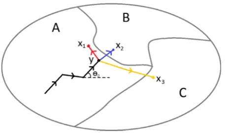
trajectoryh0and weightswij=W(Hi,Hj) (see Fig. 1). In other words,
we aim to maximize the likelihood function
YN
n¼2
PðHðxnÞjxn1;hn1;wijÞ; eqn 8
wherex1,x2,…,xNandh1,h2,…,hNare the data on the animal’s
posi-tion and bearings, respectively, and
PðHðxnÞjxn1;hn1;wijÞ ¼ R
XidxUðxjxn1;hn1ÞW½HðxÞ;Hðxn1Þ
R
XdxUðxjxn1;hn1ÞW½HðxÞ;Hðxn1Þ;
eqn 9
whereXi¼ fx2XjHðxÞ ¼Hig.
Whilst it is, in principle, possible to calculate the maximum of the likelihood function (eqn 8) by numerically evaluating the integrals in eqn (9) for each data point, this is highly computationally intensive if the data set is large, which is often the case with GPS telemetry data. We instead choose a more efficient method that makes use of a Monte Carlo sampling procedure. For each n∊{2, 3,…,N}, where {x1,…,xN} is the set of animal locations, we sample M=100 times fromΦ(x|xn1,hn1) to give a setSnof possible next
animal positions, disregarding the biasing effect that resources have on the movement. The reason for usingM=100 is to reduce com-putational time for analysing our large data set (>300 000 steps), and by examining a small subset of the data using M=1000, we obtain similar results toM=100. We then use the approximation
R
XidxUðxjxn1;hn1Þ jfs2SnjHðsÞ ¼Higj=jSnjto give
PðHðxnÞjxn1;hn1;wijÞ ¼ R
XidxUðxjxn1;hn1ÞW½HðxÞ;Hðxn1Þ
P
j
R
XjdxUðxjxn1;hn1ÞW½HðxÞ;Hðxn1Þ W½HiP;Hðxn1Þjfs2SnjHðsÞ ¼Higj
s2SnW½HðsÞ;Hðxn1Þ
;
[image:4.595.63.292.478.613.2]eqn 10
where |S| denotes the number of elements in a setS, so that the likelihood function is
LðwijÞ ¼
YN
n¼2
W½Hi;Hðxn1Þjfs2SnjHðsÞ ¼Higj P
s2SnW½HðsÞ;Hðxn1Þ
: eqn 11
To maximize eqn (11) efficiently, we split it into several likelihood functionsLj, one for each habitat typeHj
LjðwijÞ ¼ Y n12Qj
wijjfPs2SnjHðsÞ ¼Higj
s2SnW½HðsÞ;Hj
; eqn 12
whereQjis the set of indicesmsuch thatH(xm)=Hj. For eachj, we
maximize the corresponding likelihood function (eqn 12) indepen-dently of the others, whilst ensuring thatwjj=1, using the Nelder–
Mead simplex algorithm (Lagariaset al.1998), as implemented in the Pythonmaximize()function from the SciPy library (Jones, Oli-phant & Peterson 2001). The likelihood function for the entire data set is simply the productLðwijÞ ¼QjHjj¼1LjðwijÞ, wherejHjis the number of habitat types. To obtain error bars for the weights, we bootstrapped the set of steps 100 times and calculated the maximum likelihood parameter values for each. Error bars are standard deviations of the results.
NU MER ICAL IN V ES TIGATION O F TH E M ODEL
To investigate the model, we constructed artificial resource landscapes on a 50 by 50 square lattice, where the lattice spacing is 200 m. We used the weighting functionW(Hi,Hj), step length and turning angle
distri-butions found by fitting to the caribou data, as described in the previ-ous subsection. We computed the steady-state position distribution numerically on this lattice by iterating the master equation (eqn 3) through time until |u(x,h,t+dh)u(x,h,t)|<108for every value ofxandh.
To understand how patch size and isolation affect the steady-state probability distribution, we used artificial landscapes where the left-hand half is wetland habitat and all of the right-left-hand half is coniferous
Fig. 1.Schematic representation of the movement model. The animal represented here has moved to pointyon the trajectory given by the black lines in an environment with three resource types: A, B and C. Suppose that C is the most preferable habitat for the animal, followed by A, with B being resource poor. Three of the many possible next steps for the animal are tox1,x2orx3. In the absence of a resource response,
and assuming that the animal is a correlated walker with a step length distribution that decays with increasing distance, the most likely move would be tox2in patch B. However, due to the poor quality of patch B,
the animal may instead decide to take a sharp left turn to stay in patch A (represented by a move tox2) or even to take a sharp right turn and
dense forest, except for a small square of wetland, which we callthe patch. The reason for having the left-hand half of the terrain as good-quality wetland habitat is that animals need to be given a choice between a small patch and a large contiguous area of good habitat. If the terrain contains just a single good patch on its own in the middle of poor habitat, then the animals will choose the good patch with high probability even if it is small and isolated, as it is the best option avail-able. We also used the same step length and turning angle distribution in both habitats, so as to isolate the effect of the weighting function on space use patterns.
To investigate the patch size effect, we placed the patch 12 km to the right of the centre of the landscape and halfway up. We varied the patch size from 016 to 784 km2. To make sure that the overall amount
of wetland and forest was the same in each artificial landscape, we replaced a strip of wetland on the left-hand side of the landscape with coniferous dense forest, ensuring that the area of the strip was the same as that of the patch. To examine the isolation effect, the patch was placed at differing distances to the right of the landscape centre, between 04 and 32 km, and the patch size was kept constant at 16 km2.
Results
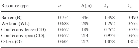
We identified five different habitat types within the landscape: wetland (WL), barren (B), dense coniferous forest (CD), open coniferous forest (CO) and other (O). The O category consists of water and other non-abundant resources, such as byroids, herbs and broadleaf. For all of these habitats, the bivariate von Mises distribution for the turning angles and the Weibull distri-bution for the step lengths were good fits to the data (Fig. 2, Table 1).
The best-fit parameters for the weighting function W(Hi,Hj) are shown in Table 2. This table suggests that WL should be the most favourable habitat type, since the weight given to moving there from other habitats is always>1. B is close behind, being preferable to all other habitats except wet-land. CO is a middling habitat, with half the weights of moving there being>1 and the other half less. CD appears to be nota-bly less preferable to these first three, with O being the least favourable of all categories.
When a small WL patch is placed in the midst of an area of CD, in the simulated environment described in the methods section, the average space use per unit area increases with the size of the patch but decreases with isolation (Fig. 3), showing the effect of the weighting function on the emergent space use patterns. However, variations in step length and turning angle distributions also play an important role. The further an ani-mal moves between fixes, the faster it is moving on average, which affects the animal’s space use distribution. Previous mechanistic models (Moorcroft, Lewis & Crabtree 2006; Moorcroft & Lewis 2006) have shown that some animals, for example coyote (Canis latrans) (Laundre & Keller 1981), will decrease their speed of movement in more favourable habitats and that this causes them to be observed with higher probabil-ity in better habitats than worse ones. However, in certain cir-cumstances, some species, for example elk (Cervus elaphus) (Anderson, Forester & Turner 2008) and black bears (Ursus americanus) (Bastille-Rousseauet al.2011), do not appear to slow down in preferred habitats.
Similar to these latter examples, the caribou in our study move fastest in habitats B and WL (Table 1), most likely because these habitats are open and offer relatively few obstructions to movement for a large and long-legged animal such as caribou. However, B and WL appear from the resource weightings (Table 2) to be preferable to the other three habi-tats. Since the faster movement in B and WL would cause the caribou to spend relatively less time in these habitats than would be expected if all the step length distributions were equal, we have competing effects between fidelity to these habi-tats due to the tendency to move into these habihabi-tats from oth-ers and lower space use caused by faster moving within B and WL.
To examine these competing effects, we computed numeri-cally the steady state of the ME (eqn 3) in an artificial land-scape consisting of just WL and CD habitat types (Fig. 4a). These are chosen because animals move fast in WL (Table 1) but it is the most preferential habitat according to the weight-ing function (Table 2), whereas animals move slowly in CD but do not choose this habitat preferentially over WL, B or CO. When the step length distributions for both habitats are the same (Fig. 4b), there is a clear preference for WL. In addi-tion to this, the probability density is highest in the largest con-tiguous WL area, towards the bottom-left than in the other, smaller patches. The smallest patches of WL, in the top-left and top-right, show the lowest probability density of all the WL patches. This is a feature of space use that does not emerge in the mechanistic resource selection model of Moorcroft & Barnett (2008). In that model, the space use at any point is a function of the resource quality at that point, so that the prob-ability density would be of the same magnitude in all the WL patches. Here, the preference of animals for large, contiguous patches of high-quality habitat emerges naturally from the underlying movement processes.
[image:5.595.58.289.567.647.2]When we solve the steady state of the ME (eqn 3) in the same landscape, but this time with different step length distri-butions in different habitat types, as given in Table 1, very dif-ferent space use patterns emerge (Fig. 4c). CD is much more
Table 1. Step lengths and turning angles for the caribou data
Resource type a b(m) k1 k2
Barren (B) 0754 346 1498 0490 Wetland (WL) 0688 289 1292 0573 Coniferous dense (CD) 0677 189 0762 0733 Coniferous open (CO) 0677 214 0933 0673 Others (O) 0604 212 1028 1057
(a) (b)
(c) (d)
(e) (f)
[image:6.595.65.435.67.750.2](g) (h)
Table 2. Resource weights for the caribou data
From to B to WL to CD to CO to O
Barren (B) 100 105001 063002 089001 041001 Wetland (WL) 095001 100 064001 093001 038001 Coniferous dense (CD) 117004 108002 100 106001 035001 Coniferous open (CO) 107001 107001 082001 100 029001 Others (O) 165005 164005 092005 138004 100
The weightingW(Hi,Hj) given to travelling from one habitatHjto anotherHi, calculated from the caribou data.W(Hi,Hj)>1 means thatHiis
preferable toHj, whereas movement from a more preferable habitat to less meansW(Hi,Hj)<1. Consequently,W(Hj,Hj)=1 for anyHj. Columns
denote the habitat type to which the animal is moving and rows denote the habitat from where the animal came. Each of the non-diagonal entries were significantly different from 1, withP<00001, using likelihood ratio test. Error bars are single standard deviations obtained by bootstrapping the data (see ‘Materials and Methods’).
[image:7.595.64.532.237.441.2](a) (b)
Fig. 3. The size and isolation of a patch affect the probability of model animals being found in the patch. Panel (a) shows the average probability den-sity of an animal to be found in a (good quality) wetland patch surrounded by (poor quality) dense coniferous forest, as a function of the size of a patch in km2. Panel (b) shows the same average probability density, this time as a function of the distance of the patch inkmfrom a large contiguous area of
wetland (see ‘Materials and Methods’ for details). In both panels, the solid lines show the results of the steady-state solution of the model described in this study. The dashed lines show the results of the steady-state solution of the model described in Moorcroft & Barnett (2008), when the weight of moving to wetland is 117 times that of moving to dense coniferous forest. In our model, mean probability density increases with patch size and decreases with patch isolation, whereas neither of these properties of the patch have an effect on the animal probability density in Moorcroft & Barnett’s model.
(a) (b) (c)
[image:7.595.61.535.534.693.2]preferable in this scenario than that in Fig. 4b. Particularly, the centre of the large contiguous area of CD in the top-right has the highest probability density of the whole landscape. Here, the animals are far away from any WL habitat, and mov-ing slowly, so are less likely to choose preferentially to travel to the WL habitat than stay in the same patch. The only other place where the probability density is as high as in the centre of the large CD area is the small WL patch at the top-right, which is the only patch of WL near the centre of the CD habitat. Con-versely, the isolated patch of CD in the bottom-left, sur-rounded by a large area of WL, is relatively under used, since animals there are always close to the preferable WL habitat, so will tend to move from the CD patch to the surrounding WL area.
Another interesting feature of Fig. 4c occurs along the edge of the large patch of wetland. The probability density at the edge is higher than anywhere else in this wetland patch, owing to the model animals tending to move there if they end up at the neighbouring edge of the forest. A variety of species have been observed to choose preferentially the edge of a good habi-tat over the interior, for example insects such as large white butterflies (Pieris brassicae) (Bergerotet al.2013), mammals such as pygmy tarsiers (Tarsius pumilus) (Grow, Gursky & Duma 2013) and reptiles such as black rat snakes (elaphe obsoleta obsoleta) (Blouin-Demers & Weatherhead 2001). Our model may go some way to explaining the mechanisms behind this phenomenon.
Discussion
We have constructed a mechanistic movement model, based on a step selection function (SSF), where the movement is gov-erned by the relative habitat quality between the start and the end of the step. Though simple in concept, this model has com-plex outcomes that mimic features of space use observed in many animal populations and that are not present in simpler mechanistic resource selection models (Moorcroft & Barnett 2008). As well as patch usage being correlated with local habi-tat quality, the size and isolation of the patch also affect the space use patterns that emerge from our model. Larger patches of good habitat are more likely to be used than smaller ones of equal quality. Additionally, isolated patches of good habitat inside large areas of bad habitat are less used than patches of similar size and quality that occur near bigger, good-quality patches. Both of these features of space use have been observed in a wide variety of animal populations (Andren 1994) so it is important for mechanistic models to replicate them in order to make accurate predictions.
We generalized the SSF for a correlated random walk from the version in Forester, Im & Rathouz (2009). The latter is a two-step Markov process, depending upon the position of the animal at the previous two time steps. However, in order to construct a master equation from the SSF (Moorcroft & Bar-nett 2008), it is convenient to use our one-step Markov process formulation, which depends upon the position and bearing at the previous time-step (eqn 1). We also extended the SSF from Forester, Im & Rathouz (2009) to enable inclusion of
information about the whole step, as done in Fortin et al. (2005), rather than just the end of the step. A strength of the master equation approach is that it gives the full probability distribution as it evolves over time by solving the equation just once. Since it is not subject to random variation, as is the case when performing stochastic simulations, this obviates the need for simulating multiple realizations or having to determine how many simulations are required to give a full and accurate picture of the model behaviour.
We have explained how to parametrize our model from location data, using herds of caribou in Newfoundland as our test population. This advances the study of Moorcroft & Bar-nett (2008), which describes purely theoretical results in a mathematically simplified one-dimensional world, and will enable biologists to construct mechanistic step selection mod-els appropriate for their study species. Whilst we have focused on resources in the present paper, our model can be readily extended to include other environmental covariates. Such models could be used to test hypotheses about the mechanisms that cause observed space use patterns to emerge in the popula-tion (Moorcroft, Lewis & Crabtree 2006).
Resource selection techniques have been successfully used to uncover the driving factors behind movement decisions for a large variety of populations (Manly et al. 2002). However, they cannot, by themselves, relate movement decisions to spatially explicit, population-level patterns of usage in a non-speculative, analytic fashion. Mechanistic models, on the other hand, were developed precisely for this reason: to derive the space use distribution of animals from details of the underlying causal processes (Moorcroft & Lewis 2006). They therefore provide a quantitative link between individual-level and popu-lation-level descriptions. This is vital for accurately building and parametrizing models that are often constructed on the population-level, such as those of disease spread and predator– prey dynamics, but whose underlying processes are driven by individual-level movement and interaction events.
Whilst the recent development of SSFs (Fortinet al.2005; Rhodeset al.2005; Forester, Im & Rathouz 2009) has gone a considerable way towards framing resource selection in the context of the animal’s movement mechanisms, previous stud-ies have not used the SSF to determine the utilization distribu-tion that the SSF would predict. Here, we demonstrate how to frame an SSF, which can take into account features of the whole step, in such a way as to derive this utilization distribu-tion, via construction of a master equation. This gives a frame-work for studying how different environmental covariates affect space use patterns. It would therefore be possible to use our techniques to shed light on how the various covariates described in previous step selection studies each affect the way animals use space, thus giving insights into why certain parts of the landscape are used more than others and ultimately helping predict the effect of possible future landscape changes on animal space use.
the past, animal behaviour can be far more complex than cur-rent mechanistic models consider. Diffecur-rent foraging strategies can lead to an increased use of a given resource; animals can increase time spent in a patch by reducing their rate of move-ment within a patch or by selectively moving between patch of a specific type (Bastille-Rousseau, Fortin & Dussault 2010) as predicted by optimal foraging theory (Morris & Davidson 2003). The resource weighting function added to our mechanis-tic model allows explicit representation of such behaviour and may be used to enable researchers to have a better understand-ing of the foragunderstand-ing strategies animals use. Our resource weight-ing function also naturally gives rise to real aspects of animal space use such as large areas of good resource being used more intensively than smaller patches, which are important features of animal space use. This occurs by ensuring that the relative quality of the habitat between the start and end of each step is considered, so that the effect of resource quality at a point is propagated through the landscape by the non-local movement decisions of the animal.
However, the weighting function and movement parameters assume that the preference for a given resource or habitat is constant and will not change based on the spatial context that animals are currently in. This assumption may not hold when habitat selection is subject to a functional response; that is, that the selection for a specific attribute is changing with the spatial context (Mysterud & Ims 1998; Hebblewhite & Merrill 2008). Animals living in an area with different availability of resources could display different responses based on feature availability at multiple scales, such as within home range or inter home range (Moreau et al. 2012). It may therefore be necessary, when applying our mechanistic step selection model to multi-ple individuals ranging large areas, to assess first the presence of variation between and within individual behaviour based on habitat availability. Indeed, such an assessment could be made using our modelling framework. To apply the framework to a single animal requires no methodological changes, but simply applying the same techniques to the movement data for a sin-gle animal, rather than pooled data as demonstrated here. Based on the scale of the functional response, different parame-ter estimates could then be obtained for individuals experienc-ing heterogeneous conditions or for specific areas of the landscape.
The purpose of this paper is not specifically to study cari-bou behaviour. However, the fact that we have chosen data on this particular species to parametrize our model has opened up various questions about caribou space use that we hope to answer in future work. For example, why do caribou move faster in preferred habitats? It may also be interesting to compare habitat choice over longer temporal scales than two hours. If it can be shown that the choices tend to be made over longer time periods, this would suggest that the animals are using some sort of cognitive map of the environment to determine their movement, rather than simply making choices on a step-by-step basis. Furthermore, temporal differences, such as variations in night-and day-time behaviour, may have an impact on space use, which would be worth investigating in future.
On the more theoretical side, the results of this paper suggest that other choices of parameter may cause the formation of further, qualitatively different spatial patterns. Due to the inherent computational intensiveness of numerical simula-tions, rigorous and exhaustive analysis of such patterns requires development of an analytic theory of the type of SSFs studied here. Such analysis would also help illuminate the rea-sons behind the phenomena unveiled by the numerical studies of this paper. We hope to examine these ideas in future work.
The present study deals with the effect of movement pro-cesses on space use. However, interactions between animals also have an important effect in many populations, either due to collective grouping phenomena (Couzin et al. 2002; Camazineet al.2003) or territorial exclusion (Lewis & Murray 1993; Giuggioli, Potts & Harris 2011). In principle, the latter can be factored in our mechanistic modelling framework by including a term into our SSF (eqn 2) that excludes movement by animals into places recently occupied by individuals from a neighbouring group, flock or pack. Simulation analysis of sim-ilar systems, which account for territorial behaviour but not resource selection (Giuggioli, Potts & Harris 2011; Potts, Har-ris & Giuggioli 2012, 2013), shows that the resulting territories are not fixed in space. Therefore, including territorial interac-tions would require that the boundary,Ω, in the ME (eqn 3) were replaced by one that varies in time. Whilst this is not nec-essary for the caribou population modelled here, as they do not form territories, for many animals, this is an important consideration in linking individual mechanisms to the popula-tion patterns. We hope to include this in future studies.
Acknowledgements
This study was partly funded by NSERC Discovery and Acceleration grants (MAL, JRP). MAL also gratefully acknowledges a Canada Research Chair and a Killam Research Fellowship. This study was partly funded by the Institute for Biodiversity, Ecosystem Science & Sustainability and the Sustainable Develop-ment & Strategic Science Division of the Newfoundland & Labrador DepartDevelop-ment of Environment & Conservation. GBR was supported by a scholarship from the NSERC. Caribou telemetry data were provided by the Newfoundland and Lab-rador Department of Environment and Conservation. We thank all the govern-ment personnel involved in the caribou captures and monitoring over the last four decades. We are grateful to Ulrike Schl€agel and Jimmy Garnier from the Lewis Lab for helpful discussions regarding modelling and analysis, as well as two reviewers for useful comments that helped improve the manuscript.
References
Anderson, D.P., Forester, J.D. & Turner, M.G. (2008) When to slow down: elk residency rates on a heterogeneous landscape.Journal of Mammalogy,89, 105–114.
Andren, H. (1994) Effects of habitat fragmentation on birds and mammals in landscapes with different proportions of suitable habitat: a review.Oikos,71, 355–366.
Arthur, S.M., Manly, B.F.J., McDonald, L.L. & Garner, G.W. (1996) Assessing habitat selection when availability changes.Ecology,77, 215–227.
Bastille-Rousseau, G., Fortin, D. & Dussault, C. (2010) Inference from habi-tat-selection analysis depends on foraging strategies.Journal of Animal Ecol-ogy,79, 1157–1163.
Bastille-Rousseau, G., Fortin, D., Dussault, C., Courtois, R. & Ouellet, J.P. (2011) Foraging strategies by omnivores: are black bears actively searching for ungulate neonates or are they simply opportunistic predators?Ecography,34, 588–596.
Bender, D.J., Contreras, T.A. & Fahrig, L. (1998) Habitat loss and population decline: a meta-analysis of the patch size effect.Ecology,79, 517–
533.
Bergerot, B., Tournant, P., Moussus, J.-P., Stevens, V.-M., Julliard, R., Bagu-ette, M. & Foltte, J.-C. (2013) Coupling inter-patch movement models and landscape graph to assess functional connectivity.Population Ecology,55, 193–203.
Blouin-Demers, G. & Weatherhead, P.J. (2001) Habitat use by black rat snakes (elaphe obsoleta obsoleta) in fragmented forests.Ecology,82, 2882–
2896.
Borger, L., Dalziel, B. & Fryxell, J.M. (2008) Are there general mechanisms of€ animal home range behavior? A review and prospects for future research. Ecol-ogy Letters,11, 637–650.
Breed, G.A., Jonsen, I.D., Myers, R.A., Bowen, W.D. & Leonard, M.L. (2009) Sex-specific, seasonal foraging tactics of adult grey seals (Halichoerus grypus) revealed by state-space analysis.Ecology,90, 3209–3221.
Camazine, S., Deneubourg, J.-L., Franks, N.R., Sneyd, J., Theraulaz, G. & Bon-abeau, E. (2003)Self-Organization in Biological Systems. Princeton University Press, Princeton, New Jersey, USA.
Couzin, I.D., Krauze, J., James, R., Ruxton, G.D. & Franks, N.R. (2002) Collec-tive memory and spatial sorting in animal groups.Journal of Theoretical Biol-ogy,218, 1–11.
Forester, J.D., Im, H.K. & Rathouz, P.J. (2009) Accounting for animal move-ment in estimation of resource selection functions: sampling and data analysis. Ecology,90, 3554–3565.
Fortin, D., Fryxell, J.M., O’Brodovich, L. & Frandsen, D. (2003) Foraging ecol-ogy of bison at the landscape and plant community levels: the applicability of energy maximization principles.Oecologia,134, 219–227.
Fortin, D., Beyer, H.L., Boyce, M.S., Smith, D.W., Duchesne, T. & Mao, J.S. (2005) Wolves influence elk movements: behavior shapes a trophic cascade in Yellowstone National Park.Ecology,86, 1320–1330.
Gannon, W.L. & Sikes, R.S. (2007) Guidelines of the American Society of Mammalogists for the use of wild mammals in research.Journal of Mammal-ogy,88, 809–823.
Giuggioli, L., Perez-Becker, S. & Sanders, D.P. (2013) Encounter times in over-lapping domains: application to epidemic spread in a population of territorial animals.Physical Review Letters,110, 058103.
Giuggioli, L., Potts, J.R. & Harris, S. (2011) Animal interactions and the emer-gence of territoriality.PLoS Computational Biology,7, 1002008.
Grant, J.W.A. & Kramer, D.L. (1990) Territory size as a predictor of the upper limit to population density of juvenile salmonids in streams.Canadian Journal of Fisheries and Aquatic Sciences,47, 1724–1737.
Grow, N., Gursky, S. & Duma, Y. (2013) Altitude and forest edges influence the density and distribution of pygmy tarsiers (Tarsius pumilus).American Journal of Primatology,75, 464–477.
Hebblewhite, M. & Merrill, E. (2008) Modelling wildlife-human relationships for social species with mixed-effects resource selection models.Journal of Applied Ecology,45, 834–844.
Hill, J.K., Thomas, C.D. & Lewis, O.T. (1996) Effects of habitat patch size and isolation on dispersal byHesperia commabutterflies: implications for meta-population structure.Journal of Animal Ecology,65, 725–735.
Houston, A.I., Higginson, A.D. & McNamara, J.M. (2011) Optimal foraging for multiple nutrients in an unpredictable environment.Ecology Letters,14, 1101–
1107.
Hurford, A. (2009) GPS measurement error gives rise to spurious 180°turning angles and strong directional biases in animal movement data.PLoS ONE,4, e5632.
Jones, E., Oliphant, T., Peterson, P.,et al.(2001)SciPy: Open Source Scientific Tools for Python. URL: http://www.scipy.org/.
Kenkre, V.M., Giuggioli, L., Abramson, G. & Camelo-Neto, G. (2007) Theory of hantavirus infection spread incorporating localized adult and itinerant juve-nile mice.European Physical Journal B: Condensed Matter and Complex Sys-tems,55, 461–470.
Lagarias, J.C., Reeds, J.A., Wright, M.H. & Wright, P.E. (1998) Convergence properties of the Nelder-Mead simplex method in low dimensions.SIAM Journal on Optimization,9, 112–147.
Laundre, J.W. & Keller, B.L. (1981) Home-range use by coyotes in Idaho.Animal Behaviour,29, 449–461.
Lewis, M.A. & Murray, J.D. (1993) Modelling territoriality and wolf-deer inter-actions.Nature,366, 738–740.
Mahoney, S.P. & Schaefer, J.A. (2002) Long-term changes in demography and migration of Newfoundland caribou.Journal of Mammalogy,83, 957–963. Manly, B. (1974) A model for certain types of selection experiments.Biometrics,
30, 281–294.
Manly, B.F., McDonald, L.L., Thomas, D.L., McDonald, T.L. & Erikson, W.P. (2002)Resource Selection by Animals: Statistical Design and Analysis for Field Studies, 2nd edn. Chapman and Hall, New York, NY, USA.
McIntyre, N.E. & Wiens, J.A. (1999) Interactions between landscape structure and animal behavior: the roles of heterogeneously distributed resources and food deprivation on movement patterns.Landscape Ecology,14, 437–447. McKenzie, H.W., Merrill, E.H., Spiteri, R.J. & Lewis, M.A. (2012) Linear
fea-tures affect predator search time: implications for the functional response. Journal of the Royal Society Interface Focus,2, 205–216.
Moorcroft, P.R. & Barnett, A. (2008) Mechanistic home range models and resource selection analysis: a reconciliation and unification.Ecology,89, 1112–
1119.
Moorcroft, P.R. & Lewis, M.A. (2006) Mechanistic Home Range Analysis. Princeton University Press, Princeton.
Moorcroft, P.R., Lewis, M.A. & Crabtree, R.L. (2006) Mechanistic home range models capture spatial patterns and dynamics of coyote territories in Yellow-stone.Proceedings of the Royal Society, Series B,273, 1651–1659.
Moreau, G., Fortin, D., Couturier, S. & Duchesne, T. (2012) Multi-level func-tional responses for wildlife conservation: the case of threatened caribou in managed boreal forests.Journal of Applied Ecology,49, 611–620.
Morris, D.W. & Davidson, D.L. (2003) Optimally foraging mice match patch use with habitat differences in fitness.Ecology,81, 2061–2066.
Mysterud, A. & Ims, R.A. (1998) Functional responses in habitat use: availability influences relative use in trade-off situations.Ecology,79, 1435–1441. Potts, J.R., Harris, S. & Giuggioli, L. (2012) Territorial dynamics and stable home
range formation for central place foragers.PLoS ONE,7, e34033.
Potts, J.R., Harris, S. & Giuggioli, L. (2013) Quantifying behavioral changes in territorial animals caused by sudden population declines.The American Natu-ralist,182, E73–E82.
Rhodes, J.R., McAlpine, C.A., Lunney, D. & Possingham, H.P. (2005) A spa-tially explicit habitat selection model incorporating home range behavior. Ecology,86, 1199–1205.
Wulder, M.C., White, J.C., Cranny, M., Hall, R.J., Luther, J.E., Beaudoin, A., Goodenough, D.G. & Dechka, J.A. (2008) Monitoring Canada’s forests. Part 1: completion of the EOSD land cover project.Canadian Journal of Remote Sensing,34, 549–562.
Received 18 May 2013; accepted 2 December 2013 Handling Editor: Sean Rands
Supporting Information
Additional Supporting Information may be found in the online version of this article.
[image:10.595.64.309.70.655.2]Appendix S1.Implementing eqn (3) from the main text in discrete space.