The Sphereprint: An approach to quantifying the conformability of flexible materials

White Rose Research Online URL for this paper: http://eprints.whiterose.ac.uk/87732/

Version: Accepted Version

Article:

Sageman-Furnas, AO, Goswami, P, Menon, G et al. (1 more author) (2014) The Sphereprint: An approach to quantifying the conformability of flexible materials. Textile Research Journal, 84. 793 - 807. ISSN 0040-5175

https://doi.org/10.1177/0040517513512402

[email protected] https://eprints.whiterose.ac.uk/

Reuse

Unless indicated otherwise, fulltext items are protected by copyright with all rights reserved. The copyright exception in section 29 of the Copyright, Designs and Patents Act 1988 allows the making of a single copy solely for the purpose of non-commercial research or private study within the limits of fair dealing. The publisher or other rights-holder may allow further reproduction and re-use of this version - refer to the White Rose Research Online record for this item. Where records identify the publisher as the copyright holder, users can verify any specific terms of use on the publisher’s website.

Takedown

If you consider content in White Rose Research Online to be in breach of UK law, please notify us by

conformability of flexible materials

Andrew O Sageman-Furnas1, Parikshit Goswami1, Govind Menon2 and Stephen J Russell1

Abstract

The Sphereprint is introduced as a means to characterize hemispherical conformability, even when buckling occurs, in a variety of flexible materials such as papers, textiles, nonwovens, films, membranes and biological tissues. Conformability is defined here as the ability to fit a doubly curved surface without folding. Applications of conformability range from the fit of a wound dressing, artificial skin, or wearable electronics around a protuberance such as a knee or elbow to geosynthetics used as reinforcements.

Conformability of flexible materials is quantified by two dimensionless quantities derived from the Sphereprint. The Sphereprint ratio summarizes how much of the specimen conforms to a hemisphere under symmetric radial loading. The Coefficient of Expansion approximates the average stretching of the specimen during deformation, accounting for hysteresis. Both quantities are reproducible and robust, even though a given material folds differently each time it conforms.

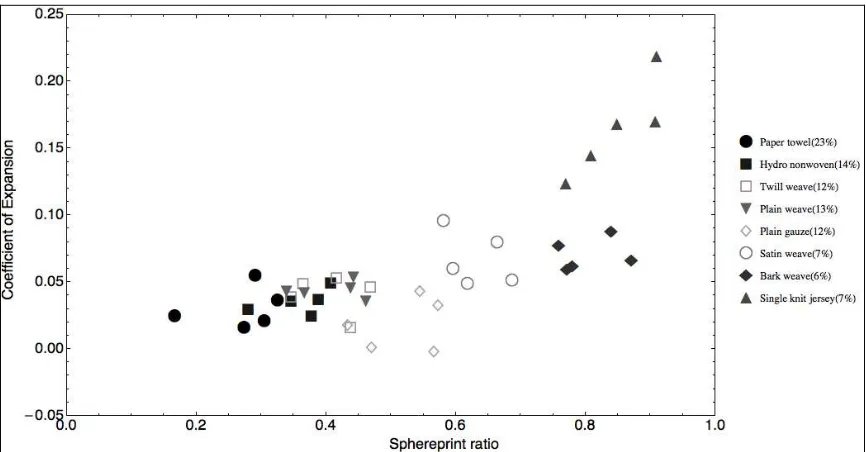
For demonstration purposes, an implementation of the Sphereprint test methodology was performed on a collection of cellulosic fibrous assemblies. For this example, the Sphereprint ratio ranked the fabrics according to intuition from least to most conformable in the sequence: paper towel, plain weave, satin weave, and single knit jersey. The Coefficient of Expansion distinguished the single knit jersey from the bark weave fabric, despite them having similar Sphereprint ratios and, as expected, the bark weave stretched less than the single knit jersey did during conformance.

This work lays the foundation for engineers to quickly and quantitatively compare the conformance of existing and new flexible materials, no matter their construction.

Keywords

Sphereprint, conformability, material characterization, flexible material, textiles, nonwovens

1

Centre for Technical Textiles, School of Design, University of Leeds, Leeds, LS2 9JT, UK

2

Division of Applied Mathematics, Brown University, Providence, RI, 02912, USA

Corresponding author:

Andrew O Sageman-Furnas, Centre for Technical Textiles, School of Design, University of Leeds, Leeds, LS2 9JT, UK.

Introduction

Engineering flexible materials to conform to the shapes around us is an important problem in materials science. High performance applications, with an emphasis on deformability of shape, range from tissue scaffolding and organ reinforcement to

geosynthetics for membrane protection in landfills and for soil reinforcement. The way in which textiles for wound dressings, wearable electronics and garment technologies fit a fingertip, elbow or knee is also dictated by the flexible materials' ability to conform. Amongst all materials, textiles are best known for their ability to attain different shapes through in-plane straining and nearly reversible buckling1, familiarly known as stretching and folding/unfolding, respectively. Therefore, historically, research on the attainment of complex shapes by flexible materials has been mostly constrained to textiles and in particular to garment technology. In this particular field, there has been considerable work done on drapeability and its quantification by some form of Drapemeter2,3.

Informally, drapeability is the ability of a textile to fall in graceful folds under gravity as in the hanging of curtains, the flow of a skirt over the body, or the hanging edge of a table cloth4. General theories on the geometry of buckling and on the elements of draping under gravity have been investigated5,6. However, with the introduction of flexible electronics7,8 and artificial skins9,10 that either mimic or explicitly incorporate a textile structure to ensure acceptable conformability; flexible textile composites in place of more traditional engineering materials; and the importance of wearable, single-use nonwoven products in the consumer and healthcare markets, it is increasingly necessary to quantify flexible material shape attainment in other contexts and at different scales.

While the collection of all shapes may seem intractable, two dimensional surfaces can be classified into a few distinct categories based on curvature. Every piece of a surface can be considered as flat, singly or doubly curved11. Flat pieces are like tabletops. Singly curved pieces are like cylinders e.g. the label of a tin can. Doubly curved pieces come in two types: those which resemble parts of a sphere or ball, and those which resemble a saddle. Balls are doubly curved in the same direction, for example both up like at the south pole of the Earth or both down, like at the north pole. A saddle is doubly curved with one curve going up, to keep the rider in the saddle, and the other curve going down, to accommodate the legs. Many textiles easily conform to large regions of double curvature. This conformability is in stark contrast to paper or other sheet materials or metals which cover flat or singly curved shapes easily, but crease or fracture during conformation to a shape which is doubly curved. From the perspective of curvature, quantifying how a nonwoven wound dressing conforms to a knee is similar to quantifying how a geosynthetic membrane conforms to the bottom of a landfill.

uniaxial stretch and recovery test. Specimens are marked at two points, extended twenty percent using a tensile testing machine, held for sixty seconds and then relaxed for three hundred seconds. Thus, the test records extensibility and permanent elongation sets17, possibly in multiple directions. A definition of forced conformability in relation to

nonwovens has also been proposed18. This definition matches with the understanding that conformability is the ability of a material to fit a doubly curved surface. However,

descriptions of the exact testing procedure and the device itself have been limited18. Conformability has appeared in studies of flat tape woven structures19 and artificial skin9, but only minimal quantification is provided, with most of the emphasis on visual

comparison. In the field of composites, issues related to the formability and molding of fibrous assemblies around spherical objects have been extensively discussed20-27. While many of these studies are interested in the hemispherical conformability of textiles for shape attainment, forming is an irreversible process in which folds are defects and so this flexible nature in the final material is forgotten. The Drapability test from Rozant et al.26, for wovens and knits to be used in composite forming, uses a hemispherical punch to displace a clamped, initially planar specimen, but continues only until the formation of the first fold. This ignores the important characteristic of textiles to deform in reversible buckling during shape attainment.

Conformability is defined in the present work as the ability of a flexible material to fit a doubly curved surface without folding. From the mathematical classification of surfaces, conformability to a sphere and conformability to a saddle are distinct. This study proposes a simple test method, the Sphereprint test, for quantifying the

hemispherical conformability of flexible materials using a hemisphere. Analysis is based on a visualization called the Sphereprint. The Sphereprint is thought of as the footprint on the flexible material as it conforms to the hemisphere. Two reproducible quantities are introduced: the Sphereprint ratio, which summarizes hemispherical conformability in a single value ranging from zero (low conformability) to one (perfect conformability), and the Coefficient of Expansion, a measurement of the average extension in every direction during deformation. As a demonstration of the method a Sphereprint test is implemented and a collection of cellulosic fibrous assemblies including paper, nonwoven, knits and wovens are tested.

Measuring principles

The important elements of a Sphereprint test are shown in Figure 1. They are: symmetric radial loading of the specimen onto the hemisphere, ensuring that the center of the

specimen is aligned with the north pole; taking measurements of the conformed region on the hemisphere, even when buckling may have occurred; removing the specimen from the hemisphere and unfolding it; taking measurements of the corresponding post-conformed region.

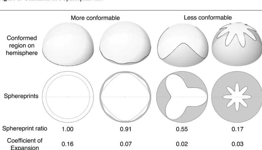
Information from a typical Sphereprint test on four materials with varying

the enclosing circle. The Coefficient of Expansion captures the average amount of extension in each direction.

A visual study of the deformation of the dotted post-conformed lines to the solid hemispherical lines provides some insight into the anisotropy of the sample material. It is simpler to understand the deformation in materials of high conformance. For example, in the left-most Sphereprint the dotted line is a circle and the solid line is simply a larger circle. This corresponds to an isotropic material, which stretches the same in each direction during conformance. The Coefficient of Expansion completely characterizes this type of behavior. The second Sphereprint from the left has a dotted line that looks like a rounded rectangle, while its solid line is wavy around the edges. The distance between the dotted line and the solid line is small along the horizontal and vertical axes, but much larger in the diagonal directions. This corresponds to the behavior of some woven materials that do not stretch much along the two x-y perpendicular directions, but do stretch along the bias, during conformance. It is more difficult to gain any insight into material anisotropy from the two right-most, less conformable, Sphereprints.

Implementation of a Sphereprint test procedure and analysis

The Sphereprint method is a general test procedure whose principles have been outlined in Section Measuring principles. The Sphereprint test procedure in the present

implementation is ten steps, which are summarized below. The text shown in italics, inside parentheses, are suggestions for implementation and state what was done for the present implementation. More explicit implementation details follow. For demonstration purposes, an array of cellulosic fibrous assemblies was characterized with the present Sphereprint test implementation. Similar implementation, data collection, and analysis techniques could be used for films, membranes, flexible composites, or biological tissues.

Step 1. Cut circular specimens (110 mm diameter) and mark the center and an axis of orientation (e.g. the machine, warp, or wale direction).

Step 2. Flatten specimens to remove creases or wrinkles (apply 2 kg, with surface area covering the entire specimen, for 4 hours).

Step 3. Place the specimen so that the center aligns with the north pole and the axis of orientation is in the 0¼ direction.

Step 4. Fix the center of the specimen to the north pole and lower the ring (hose clamp) until the top of the ring is in line with the equator.

Step 5. Dot the apex of each fold proceeding in the counterclockwise direction from 0¼. Place a circle around the first dot marked.

Step 6. Measure the caliper distance from the north pole to each dot, starting with the circled dot and progressing counterclockwise.

Step 7. For large lunes of conformance (dots which differ by more than 45¼), recursively dot the equator at the angular midpoints.

Step 8. Remove the specimen from the hemisphere and attempt to flatten it (tap the specimen 5 times on each side).

Step 9. Measure the angle between the rays from the center to neighboring dots, starting and ending with the 0¼ axis of orientation.

Setup

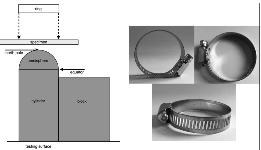
The testing device setup and nomenclature are summarized in Figure 3. A 50.8 mm diameter hemisphere (stainless steel) on a circular cylinder of the same diameter was set on the testing surface so that the axis of the cylinder was perpendicular to the testing surface. The hemisphere of diameter of 50.8 mm was chosen to mimic the size of the hemispheroidal bone segment, which protrudes during flexion of the elbow or knee. The point at the top of the hemisphere will be referred to as the north pole. The circle at the base of the hemisphere on top of the cylinder will be referred to as the equator. A 110 mm diameter circular specimen was cut out and marked at its center and along a diameter to provide an axis of orientation. This axis of orientation was aligned with a meaningful direction, such as the machine direction for papers and nonwovens, the wale direction for knits and the warp direction for wovens. The specimen was coerced to conform to the hemisphere by lowering a ring of adjustably increasing diameter from the north pole down to the equator. To prevent movement, the center of the specimen was held against the north pole of the hemisphere as the ring was lowered. A circular hose clamp was used as the ring. The hose clamp is built from a flat belt, which is 12.7 mm wide and 1 mm thick, wrapped into a cylinder with a screw through which the belt passes to allow the diameter to change. Photographs of the hose clamp are shown in Figure 3. The hose clamp is sold as a 25 mm - 51 mm clamp, but is actually extendable to 55 mm. The extra allowable 4 mm of diameter is essential since this is the range used during testing. Note also that since the diameters of interest are near the maximum dimension of the hose clamp, the overlap of the belt is minimized, allowing for a more evenly applied load. The screw of the hose clamp was always aligned perpendicular to the axis of orientation. During lowering, the ring diameter was changed as required to allow materials of

different thicknesses to be tested and to pass over folds that may form during testing. The clamp was lowered until the top of the clamp was in line with the equator. In practice, a small block was used to prevent the clamp from lowering any further.

Measurement

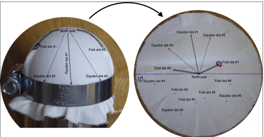
Materials that do not conform entirely to the hemisphere fold as the ring is lowered. Once the ring has been secured at the equator, the apex of each fold is dotted precisely where it lifts away from the surface of the hemisphere, see Figure 4. It is imperative that the specimen lies along the surface of the hemisphere from the north pole to the fold dot. This assertion allows the arc length between the north pole and the fold dot to be calculated from the measured linear caliper distance, as shown in Figure 4.

Observe that the fold dots section the hemisphere into a series of lunes with lune angles given by the angular differences between fold dots. If a specimen conforms completely to the hemisphere there are no fold dots to measure, so a system of marking along the equator is adopted for large lunes of conformance. Large lunes of conformance are defined by lune angles greater than 45¼. Equator dots are recursively placed along the equator at the angular midpoints between existing dots as shown in Figure 5. This ensures that all lune angles are less than 45 degrees.

First the location of each of the two fold dots extended to the equator is found; One can hold the tape measure taught from the north pole to the equator, ensuring the line of measurement passes through the fold dot. The tape measure can then be wrapped around the ring, at the equator, between the two equatorial extensions of the fold dots. As the tape measure is marked with distance, the midpoints are found by recursively dividing the length in two. This is continued until the distances between neighboring points is less than 20 mm, corresponding to an angle of 45¼ on a hemisphere of diameter 50.8 mm. If a specimen conforms completely, then eight equator dots are made in perfect symmetry about the marked axis of orientation.

The equator dot system also provides the experimenter with full discretion as to whether very small folds near the equator should be marked. A good rule of thumb seems to be to ignore folds whose caliper distances from the equator do not exceed 4 mm, roughly 4.5¼ from the equator. Note the caliper distances between the north pole and the equator dots are never measured as the equator dots by definition always lie along the equator. The spherical distance is thus equal to one quarter the length of the equator itself, 50.8π / 4 mm, since the testing hemisphere in this implementation has a diameter of 50.8 mm. The specimen is then removed from the hemisphere and placed on the testing surface. The angle between the axis of orientation and the first circled fold or equator dot is measured followed by the angles between each consecutive pair of dots. Measuring 180¼ at a time, instead of the angles between dots, may prevent angle error from accumulating, however it was observed that the post-conformed specimens may not lie flat on the table to allow for the entire 180¼ measurement to be made. The last angle measured is between the final dot and the 0¼ direction of the axis of orientation. For each fold or equator dot the post-conformed planar length to the center of the specimen is also measured, ensuring that the material lays flat against the testing surface along the line of measurement.

Analysis

The exact spherical lengths were calculated from the measured caliper distances using the equation shown in Figure 4. In practice, the sum of the measured angle differences does not add up to 360¼. The error is distributed evenly amongst the angle measurements. The angle sum is subtracted from 360¼ and then divided by the number of measured angles and the result added to each of the measured angles. For example, if there were ten measured angles adding up to 358¼, two degrees short of the full 360¼, then two tenths of a degree is added to each angle. Hereafter the dot angles referred to are accumulated measured angles adjusted by having the error uniformly distributed via this process. For example the angle corresponding to fold dot five is the sum of the first five angle differences yielding the indicated angle, α, from the axis of orientation. Each of these dot angles is paired with its corresponding spherical length and post-conformed linear length. The data points are linearly interpolated in rectangular coordinates, wrapping from 360¼ to 0¼, as shown in Figure 6 yielding the two functions sph(α)and pc(α), respectively. The Sphereprint is these two functions plotted in polar coordinates inside of the enclosing circle.

number obtained by dividing the area of the conformed region by the area of the enclosing circle. The Sphereprint ratio, area of the conformed region and area of the enclosing circle are given as equations (3), (2), and (1), respectively. These equations include the necessary constants for angles to be measured in degrees. The quantity _ris the hemispherical distance from the north pole to the equator and equals one fourth the length of the equator itself (here _r = 50.8π / 4 mm). The sph(α) and pc(α) have units of length (mm).

Area of the enclosing circle = π_r2

. (1)

Area of the conformed region = π 180

1

2sph(α) 2

dα

0 360

∫

Sphereprint ratio = Area of the conformed region

Area of the enclosing circle . (3)

The area of the enclosing circle represents perfect hemispherical conformability. It is the value calculated from following the test procedure on a specimen that conforms perfectly to the hemisphere with no folds at all. In this situation all dots are equator dots, so the solid curve will coincide with the enclosing circle. Note that the area of the enclosing circle is not the surface area of the hemisphere, but rather the area of the hemisphere under the azimuthal equidistant projection from the north pole.

The Sphereprint ratio is near zero when many fold dots are close to the north pole, representing poor conformance, and is equal to one precisely when there are no fold dots at all, representing perfect conformance. Recall, however, that the dot angles are not spherical lune angles, but rather the planar post-conformed angles after the specimen has been removed from the hemisphere and flattened. The lune angle between large folds may be small, but when unfolded back into the plane the difference in dot angle may be large. While only an approximation these planar angles can be simply and reliably measured. They were also chosen because they satisfy the property that when large swaths of material are used to create a fold, the unfolded planar angle increases, resulting in a decrease in the Sphereprint ratio.

Coefficient of Expansion = π

180 log

sph(α) pc(α) dα

0 360

∫

The summary diagram for the Sphereprint test is the Sphereprint. It is a polar plot of sph(α)and pc(α) inside of the enclosing circle, with the marked axis of orientation. An example is shown in Figure 6. Both the Sphereprint ratio and the Coefficient of Expansion are intentionally defined in terms of ratios so that they are independent of scale. With a bit of effort all test data, up to scaling, can be recovered from any of these diagrams. The cusps in the Sphereprint correspond to fold dots.

Sphereprint test results

As a demonstration of the Sphereprint method, two experiments with the present implementation of Section Implementation of a Sphereprint test procedure and analysis were performed. The material characterization experiment tests the ability of the Sphereprint to characterize the conformance of a set of example flexible materials: a range of fibrous assemblies. The reproducibility experiment tests that the procedure and analytical techniques are both reproducible and robust.

Material characterization

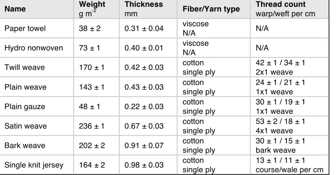
Eight fibrous assemblies of varying constructions, summarized in Table 1, were tested. For each sample, five circular specimens of diameter 110 mm were cut. The center of each specimen was marked, as was the axis of orientation, here corresponding to the warp, machine or wale direction, for wovens, nonwovens and knits, respectively. To remove wrinkles and creases, specimens were pressed (2 kg) for at least four hours prior to testing. The Sphereprint test as outlined in Section

Implementation of a Sphereprint test procedure and analysis was performed on each of the forty

Figure 8. The coefficient of variation of the Sphereprint ratio for each sample is also shown. The coefficient of variation is not shown for the CoE as it is a signed interval quantity, instead of a ratio. The coefficient of variation can only be used on ratios.

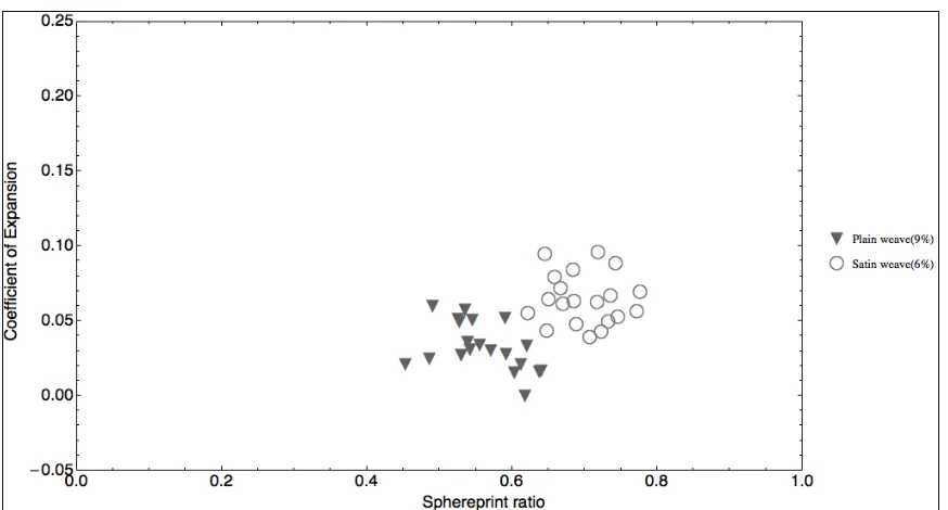
Reproducibility

To evaluate the reproducibility and assess inherent variations in both the test method and within a material, further testing was performed. Twenty specimens each of plain weave and satin weave were tested, once again face-up so that the back-face was in contact with the surface of the hemisphere, using the Sphereprint test implementation given in Section

Implementation of a Sphereprint test procedure and analysis. The data are shown in Figure 9. The coefficient of variation of the Sphereprint ratio for each sample is also shown.

Discussion

Results

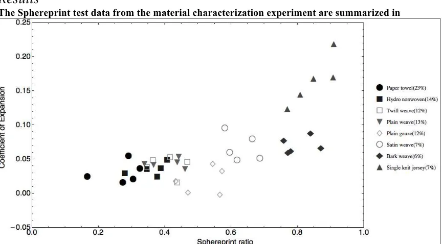
The Sphereprint test data from the material characterization experiment are summarized in

Figure 8. While the sample sizes for the characterization experiment are not large enough to perform two-dimensional statistical tests, the graphical presentation of the data

during testing, the amount of excess material below the clamp is different. This is reflected quantitatively by the two having similar Sphereprint ratios, but different CoEs. The CoE data quantify that the single knit jersey extends more in all directions during deformation than the bark weave does, so the amount of excess material below the clamp is understandably different between them. This result also matches the intuition that knits are in general more extensible than wovens, particularly when averaged over all

directions. The characterization data also suggest the anticipated positive correlation between Sphereprint ratio and CoE. However, it appeared that the bark weave and gauze materials may be outliers in this correlation as they exhibit higher Sphereprint ratios than expected from their CoEs. Such nuances of the Sphereprint test results deserve further study.

Results of the reproducibility experiment are summarized in Figure 9. The Sphereprint ratio and CoE values clearly distinguish the plain weave and satin weave from one another, as there is no overlap in the scatter of data points. Both the plain weave and satin weave data are indistinguishable from binormal distributions according to Anderson-Darling tests, summarized in Table 2. A Hotelling T-squared test suggests that the plain weave and satin weave bivariate data have different means with a p-value of 0.000014.

A visual comparison between the results of the reproducibility experiment with their counterparts from the characterization experiment suggest some differences. It appears that the plain weave and satin weave fabrics had larger Sphereprint ratios in the reproducibility experiment, despite conforming to the specifications indicated in Table 1. The coefficient of variation in the Sphereprint ratios were similar between the two data sets suggesting the differences were not due to experimental error, but rather to another experimental variable. As both samples were cellulosic, it is believed that this is

attributable to a difference in the moisture content of the second set of samples, resulting from a change in the relative humidity of the test laboratory between the first and second set of measurements.

Comparison to forced conformability

Based on the available details of the previously published test for forced

conformability18, the method and results for a few fabrics are briefly described, for purposes of comparison to the Sphereprint test. The forced conformability test uses radial loading around the edge of a 203.2 mm diameter circular specimen, on a 76.2 mm

diameter sphere. For each applied load, the distance to the first fold is measured. The first fold is defined as that closest to the north pole. The experiment continues until an

increase in load does not produce a change in the distance to the first fold. A circle is drawn on the sphere at the colatitude of the first fold. The area of the spherical cap enclosed by the circle is defined as the the forced conformability18. The Sphereprint test implementation described here uses 110 mm diameter circular specimens on a 50.8 mm diameter hemisphere. It also uses radial loading, but the load is applied by lowering a hose clamp to the equator, instead of along the edge of the specimen. The data collected for a Sphereprint contains the distance to the first fold as defined for forced

conformability value, i.e. the surface area of the spherical cap defined by the colatitude of the first fold, divided by the surface area of the hemisphere used during testing. The Firstfold ratio is dimensionless and scale independent and it is given by equation (5). Table 3 lists the materials from the paper by Shealy18 and the Sphereprint

characterization experiment with the values sorted by Firstfold ratio.

Firstfold ratio = Area of spherical cap at colatitude φ¼

Area of testing hemisphere = 1−cos(φ¼) (5)

The Sphereprint ratio and Firstfold ratio are both quantifications of hemispherical conformability. Both quantities suggest they are able to distinguish materials from each other. Table 3 compares how the Sphereprint ratio and Firstfold ratio order the

hemispherical conformability of the materials. The ordering is largely similar, however, plain gauze and single knit jersey are highlighted as they both are placed differently in the Firstfold ratio than the Sphereprint ratio. The Sphereprint ratio and Firstfold ratio penalize nonconformance differently. The Firstfold ratio strongly penalizes

nonconformance when any fold is close to the north pole, even if there are very few folds overall. In contrast, when there are only a few large folds, the Sphereprint ratio remains large. Consider plain gauze, whose Sphereprints shown in Figure 7 reveal that it often conforms with a few very large folds. This mode of conformance gives plain gauze a low Firstfold ratio but a relatively high Sphereprint ratio. Similarly, single knit jersey is penalized by the existence of any fold at all and is therefore ordered below bark weave in the Firstfold ratio ordering. Common understanding would suggest that knit jersey is very conformable and gauze has been used for many years in applications such as bandaging and in areas of wound care, where conformance to doubly curved regions of the body is required. The Sphereprint ratio quantifies hemispherical conformability in a manner more consistent with this common usage, because it takes the length of folds, number of folds and their distribution around the hemisphere into consideration. The single measurement used in computing the Firstfold ratio cannot recognize multiple modes of conformance.

Forced conformability provides an insight into hemispherical conformability. The dimensionless quantity introduced here, the Firstfold ratio, is available from the data collected in the Sphereprint test and may be useful in its own right for some applications. In particular, it is related to the quantities important for composite forming applications as described by Rozant et al.26.

Sphereprint test implementation

be collected at a later date. This should reduce testing time by more than half, since both the post-conformed angles and post-conformed lengths are required for analysis.

This Sphereprint test implementation does not include a method for measuring the force of the radial load, which may be considered a limitation. Measuring force

throughout the experiment is desirable to understand the behavior of a material during deformation and to better analyze how conformance occurs. Many quantities measured in the test depend on the relationship between stress and strain, between force and

extension. While it is shown that the Sphereprint test produces quantifiably similar results to the forced conformability test18, the forced conformability test provided a mechanism to measure the load around the edge of the specimen.

There are three difficulties in producing an improved test implementation that measures the radial force. Firstly, the mechanism must be able to apply a symmetric radial load, while also applying an appropriate amount of force at the north pole to prevent slippage of the specimen. Secondly, the ring which is lowered from the north pole to the equator must ideally be able to change in diameter while applying a

consistent, known tension to the specimen during movement. The implementation must use a ring of increasing diameter to allow radial forces to be resolved during lowering, thereby preventing fold artifacts. It was observed that small perturbations applied to the ring, as its diameter was increased while lowering, would result in a decrease in the number of folds. For example, in a few instances outside of the experiments presented here, the single knit jersey, bark weave and even the plain gauze were able to conform with no folds at all. Thirdly, the conformed hemisphere must be exposed so that the experimenter can measure the spherical distances. This precludes using a diaphragm or lining.

The Sphereprint test implementation described here fixes the cylinder with a hemispherical cap and then lowers a diameter-changing hose clamp over the specimen. Currently, the problem is that the ring is difficult to adjust while applying a known amount of force. In addition, as the ring in this implementation is a hose clamp, it does not apply a perfectly symmetrical radial load because the screw holding the circular region together breaks the symmetry. An elastomeric O-ring might be an alternative to the hose clamp. If the O-ring were of known elastic modulus, then a known amount of force would be required to change its diameter. There remains the difficulty of applying a load to the O-ring. Since motion is relative, the roles of moving and stationary pieces of the apparatus could be reversed. One could imagine an implementation in which a table had a hole which was able to change diameter, similarly to the aperture of a camera. With such an apparatus, a specimen could be placed on the table covering the aperture. A hemispherical prod would then lower by means of a simple tensile tester and the aperture would change diameter while applying tension to the specimen. Forces exerted on the specimen could be calculated from the speed of the prod and the mechanical structure of the aperture.

The technique to mark points and measure distances and angles both on the sphere and in the plane could be improved to reduce potential experimental error. Unfortunately, it is difficult to use image analysis in this context, because during

close to the equator, as is done in the current implementation. Where folds do not hide one another, an image would work well, since spherical distances could be recovered from the known projection of the visible portion of the hemisphere onto the viewing plane. An imaging technique would also allow the spherical lune angles to be calculated precisely, in addition to the post-conformed planar angles. In particular, with exact lune angles, specifying which regions are lunes of conformance would be easier. These approaches would reduce variation in the Sphereprints and the resulting Sphereprint ratios and CoEs.

Conclusion

The goal was to introduce a technique for quantifying and characterizing conformance of flexible materials to sphere-like double curvature. The general Sphereprint test method was introduced, together with a particular implementation, to understand the

hemispherical conformability of flexible materials. The Sphereprint ratio is a measure of the region of the hemisphere to which the material has conformed. While a particular material may have many ways to cover the hemisphere, the Sphereprint ratio provides a reproducible and robust summary of total conformance. The remarkable reproducibility of the Sphereprint ratio, despite the great diversity in fold patterns within a single sample material, is an interesting question for further investigation.

It has been demonstrated that the Sphereprint ratio ranks known fibrous assemblies of varying fabric construction according to conventional notions of

conformability. From least to most conformable the order was: paper towel, plain weave, satin weave, and single knit jersey. A second quantity called the Coefficient of Expansion has been introduced to understand how the flexible material behaves during conformance in relation to its post-conformed state. The Coefficient of Expansion can be thought of as a generalization of the Poisson's ratio of a material to the case of radial loading and is also reproducible and robust. It is a signed quantity, contraction cancels expansion, and the net value approximates the average extension in every direction.

The Sphereprint ratio together with the Coefficient of Expansion, provide a quantitative method to distinguish the conformance behavior of flexible assemblies. The Sphereprint itself is a visual summary of the test that contains all of the experimental data in one picture. Just as a footprint characterizes how soft clay conforms to a foot, the Sphereprint characterizes how a flexible material conforms to a sphere.

Acknowledgements

We thank Richard E. Furnas for advice on data visualization, consultation during the experimental design process, and critical reading of the manuscript.

Funding

This work was supported by a Leeds Marshall Scholarship; National Science Foundation grant DMS-0748482; Brown University; and the University of Leeds. Part of this

research was performed while A.O. S-F was at Brown University.

References

2. Chu CC, Cummings CL, Teixeira NA. Mechanics of Elastic Performance of Textile Materials: Part V: A Study of the Factors Affecting the Drape of Fabrics--The Development of a Drape Meter. Text Res J. 1950 Aug 1;20(8):539Ð548.

3. Cusick GE. The measurement of fabric drape. J Text Inst. 1968 Jun;59(6):253Ð260. 4. Hearle JWS, Grosberg P, Backer S. Structural mechanics of fibers, yarns, and fabrics.

Wiley-Interscience; 1969.

5. Cerda E, Mahadevan L. Geometry and Physics of Wrinkling. Phys Rev Lett. 2003 Feb;90:074302.

6. Cerda E, Mahadevan L, Pasini JM. The elements of draping. Proc Natl Acad Sci USA. 2004;101(7):1806Ð1810.

7. Qiao Li, Xiaoming Tao. A stretchable knitted interconnect for three-dimensional curvilinear surfaces. Text Res J. 2011 Jun 29;81(11):1171Ð1182.

8. Rogers JA, Someya T, Huang Y. Materials and Mechanics for Stretchable Electronics. Science. 2010;327(5973):1603Ð1607.

9. Chen N, Engel J, Pandya S, et al. Flexible skin with two-axis bending capability made using weaving-by-lithography fabrication method. Micro Electro Mech Syst, 2006 Istanbul. 19th IEEE Int Conf on. 2006. pp.330Ð333.

10. Someya T, Kato Y, Sekitani T, et al. Conformable, flexible, large-area networks of pressure and thermal sensors with organic transistor active matrixes. Proc Natl Acad Sci USA. 2005;102(35):12321Ð12325.

11. Stoker JJ. Differential Geometry. John Wiley & Sons, New York; 1969. p. 91. 12. Kawabata S, Niwa M. Fabric performance in clothing and clothing manufacture. J

Text Inst. 1989;80(1):19Ð50.

13. Mack C, Taylor HM. The fitting of woven cloth to surfaces. J Text Inst. 1956;47(8):477Ð488.

14. Tschebyscheff PL. Sur la coupe des v•tements. Assoc fran• pour l'avancement des sci., CongrŽs de Paris. 1878. pp.154Ð155.

15. Pipkin AC. Equilibrium of Tchebychev nets. Arch Ration Mech Anal. 1984;85(1):81Ð 97.

16. Ghys ƒ. Sur la coupe des v•tements: variation autour d'un th•me de Tchebychev. Enseign Math. 2011;57(1-2):165Ð208.

17. British Standards. 13726: Non-active medical devices Ñ Test methods for primary wound dressings Ñ Part 4: Conformability. 2003.

18. Shealy OL. Spunbonded ProductsÑA New Concept in Utilization of Fibrous Materials. Text Res J. 1965;35:322Ð329.

19. Pastore C. Conformability.

http://faculty.philau.edu/pastorec/MechTextiles/Conformability.ppt (2010).

20. Cai Z, Yu JZ, Ko FK. Formability of textile preforms for composite applications. Part 2: Evaluation experiments and modelling. Compos Manuf. 1994 Jun;5(2):123Ð132. 21. Chu TJ, Jiang K, Robertson RE. The use of friction in the shaping of a flat sheet into

a hemisphere. Polym Compos. 1996;17(3):458Ð467.

22. Hu J, Jiang Y. Modeling formability of multiaxial warp knitted fabrics on a hemisphere. Composites Part A. 2002 May;33(5):725Ð734.

complex-curvature thermoplastic composite parts. Composites. 1989;20(1):48Ð56. 25. Robertson RE, Hsiue ES, Sickafus EN, et al. Fiber rearrangements during the

molding of continuous fiber composites. I. Flat cloth to a hemisphere. Polym Compos. 1981 Jul;2(3):126Ð131.

26. Rozant O, Bourban PE, MŒnson JAE. Drapability of dry textile fabrics for stampable thermoplastic preforms. Composites Part A. 2000 Nov;31(11):1167Ð1177.

Figure 1. Schematic of a Sphereprint test.

Figure 3. Left: The Sphereprint test setup in this implementation. The ring is lowered, coercing the specimen to conform to the hemisphere, until the block prevents further movement. The block assures that the top edge of the ring is in line with the equator. The center of the specimen is aligned with the north pole.Right:The hose clamp used as the ring.

Figure 5. Left: (Step 7) A lune of conformance of angle much greater than 90¼. The fold dots are shown along with visual guides for construction lines to locate the midpoint equator dot #1 and the two recursively placed additional equator dots #2 and #3. All lune angles are now less than 45¼. Right: (Steps 8 - 10) The specimen after it has been removed from the hemisphere and flattened. Planar angle differences and planar distances from the center to each fold or equator dot can now be measured. Observe that the visual guides do not bisect the post-conformed planar angles perfectly after unfolding.

Figure 6. Left: The spherical and post-conformed linear distances as a function of dot angle, α, for each of the dotted locations along with their linear interpolations. The solid sph(α) and the dashed pc(α) are

Figure 7. Sphereprints of eight sample fibrous assemblies, five specimens per sample. The axis of orientation is shown as a faint horizontal line. The columns are sorted in increasing order of mean

Sphereprint ratio from the characterization experiment, visually evident by the increasing size of the white area in the Sphereprints going from left to right. A dashed line substantially distinguishable from its solid counterpart corresponds to a direction of strain, the average of which is given by the CoE. A cusp in a Sphereprint corresponds to the location of a fold dot. By counting cusps one can get a sense of how many folds occurred during the test.

Figure 9. Sphereprint test data collected for a reproducibility test with twenty plain weave specimens and twenty satin weave specimens. The coefficient of variation of the Sphereprint ratio is shown in parentheses next to each sample in the legend.Data distributions from the test are indistinguishable from binormal distributions. The data are visually distinct and establish a statistical difference between both the Sphereprint ratios and the Coefficients of Expansion for the plain weave and satin weave.

Table 1. Specification of fibrous assemblies utilized for experimental evaluation. Mean values and standard deviations are given for sample weight (area density), sample thickness (under 100 g of weight) and thread count based on five specimens per sample.

Name Weight g m-2

Thickness

mm Fiber/Yarn type

Thread count warp/weft per cm

Paper towel 38 ± 2 0.31 ± 0.04 viscose

N/A N/A

Hydro nonwoven 73 ± 1 0.40 ± 0.01 viscose

N/A N/A

Twill weave 170 ± 1 0.42 ± 0.03 cotton single ply

42 ± 1 / 34 ± 1 2x1 weave

Plain weave 143 ± 1 0.43 ± 0.03 cotton single ply

24 ± 1 / 21 ± 1 1x1 weave

Plain gauze 48 ± 1 0.22 ± 0.03 cotton single ply

30 ± 1 / 19 ± 1 1x1 weave

Satin weave 236 ± 1 0.67 ± 0.03 cotton single ply

53 ± 2 / 18 ± 1 4x1 weave

Bark weave 202 ± 2 0.91 ± 0.07 cotton single ply

30 ± 1 / 15 ± 1 bark weave

Single knit jersey 164 ± 2 0.98 ± 0.03 cotton single ply

13 ± 1 / 11 ± 1 course/wale per cm

Table 2. The best fit binormal distributions for the plain weave and satin weave reproducibility data. Values are shown in the format (Sphereprint ratio, CoE).

Binormal distributions Means Standard deviations Correlation Anderson Darling test p-value Plain weave (0.561, 0.032) (0.051, 0.016) -0.452 0.957 Satin weave (0.700, 0.063) (0.043, 0.017) -0.066 0.996

Table 3. Comparison between the data collected for the Sphereprint characterization experiment and the data for forced conformability18, sorted by Firstfold ratio. The data show that despite differences in testing methods the forced conformability test and Sphereprint test produce similar Firstfold ratios. The

Sphereprint ratio is also shown and orders the materials similarly with the two highlighted exceptions, plain gauze and single knit jersey. Plain gauze conforms with a few large folds which causes the Firstfold ratio to be small, while its Sphereprint ratio remains large. Single knit jersey is penalized by folds in its Firstfold ratio despite having very large lunes of conformance, and thus a large Sphereprint ratio.

Fabric type Mean Firstfold ratio Mean Sphereprint ratio High range woven* 0.495

Bark weave 0.480 0.804

High-mid range woven* 0.433

Single knit jersey 0.424 0.849 Mid range woven* 0.318

High range spunbond* 0.269

Satin weave 0.235 0.629

Plain weave 0.129 0.410

Fiber crimp B spunbond or low range woven* 0.110

Twill weave 0.105 0.407

Plain gauze 0.061 0.518

Hydro nonwoven 0.060 0.360 Fiber crimp A spunbond or starched woven* 0.057

Paper towel 0.054 0.273