Measuring the spatial accuracy of the spatial scan statistic.

(1)

promoting access to White Rose research papers

White Rose Research Online

[email protected]

Universities of Leeds, Sheffield and York

http://eprints.whiterose.ac.uk/

This is an author produced version of a paper published in

Spatial and

Spatio-temporal Epidemiology.

White Rose Research Online URL for this paper:

Published paper

Read, Simon, Bath, Peter, Willett, Peter and Maheswaran, Ravi (2011)

Measuring the Spatial Accuracy of the Spatial Scan Statistic.

Spatial and

Spatio-temporal Epidemiology, 2 (2). pp. 69-78. ISSN 1877-5845

(2)

Measuring the Spatial Accuracy of the Spatial Scan Statistic

Simon Reada_{, Peter Bath}a_{, Peter Willett}a_{, Ravi Maheswaran}b

a_{Information School, University of She}_ffi_{eld, She}_ffi_{eld S1 4DP, UK} b_{ScHARR, University of She}_ffi_{eld, She}_ffi_{eld S1 4DA, UK}

E-mail: [email protected]

Abstract

The spatial scan statistic is well established in spatial epidemiology. However, studies of its spatial accuracy are infrequent and vary in approach, often using multiple measures which complicate the objective ranking of different implementations of the statistic. We address this with three novel contributions. Firstly, a modular framework into which different definitions of spatial accuracy can be compared and hybridised. Secondly, we derive a new single measure,Ω, which takes account of all true and detected clusters, without the need for arbitrary weightings and irrespective of any chosen significance threshold. Thirdly, we demonstrate the new measure, alongside existing ones, in a study of the six output filter options provided by SaTScanTM_{. The study suggests filtering overlapping detected}

clusters tends to reduce spatial accuracy, and visualising overlapping clusters may be better than filtering them out. Although we only address spatial accuracy, the framework andΩmay be extendible to spatio-temporal accuracy.

Keywords: spatial accuracy, spatial scan statistic, benchmark testing, performance measures, Bernoulli, omega

1. Introduction

The spatial scan statistic, hereafter SSS, is a widely used tool in spatial and spatio-temporal epi-demiology. Introduced by Kulldorff and Nagarwalla (1995) and Kulldorff (1997), the purpose of the SSS is to detect the presence and location of clusters within spatial and spatio-temporal data sets. Imple-mented within the freely available SaTScanTM_software

(www.satscan.org), it has been used in well over one hundred published scholarly studies; see list in Kull-dorff(2009).

Whilst the capacity of the SSS to accurately detect the presence of clusters has been widely studied, much less so its capacity to accurately detect their location. This should be of some concern. As Kulldorff(1997) states:

... the scan statistic has the ability to identify the zone responsible for rejecting the null hy-pothesis, and if we fail to detect the real clus-ter, it is of little comfort if the null hypothesis is rejected based on an untrue cluster in an-other part of the study area.

The reason that fewer studies consider spatial (or spatio-temporal) accuracy, may be because it is not im-mediately obvious how to measure it. The literature

presents a patchwork of different measures and nomen-clatures, with the most suitable scheme dependent on the type of data used and the aims of the study. The first objective of this paper is to explore a modular frame-work into which different measures of spatial accuracy can be classified, the aim being to ease the comparison and hybridization of different measures. This is pre-sented in Section 2.

One additional complication is that most measures of spatial accuracy have multiple output parameters. This is problematic if one wishes to rank cluster detection systems in terms of spatial accuracy, without making an arbitrary choice about the relative weighting of these parameters. A second complication is that most existing measures of spatial accuracy are dependent upon an ar-bitrary choice of significance threshold. For non-spatial performance measures, a solution to both these prob-lems already exists in the form of the two-alternative-forced-choice (hereafter 2AFC) test. The 2AFC test forms the basis of the area under curve (AUC) mea-sure used with receiver operating characteristic (ROC) curves, providing a single performance measure that is independent of significance threshold, or the relative weighting of sensitivity and specificity.

(3)

straightforward 2AFC test, which is customised for the spatial scan statistic. We provisionally call thisΩ; a full definition and derivation are presented in Section 3.

The final objective of this paper is to provide a brief, but useful demonstration, of the new Ω measure. To this end, the six different output filtering options pro-vided by SaTScanTM _{are evaluated in terms of their}

ef-fect on spatial accuracy. This is done using the Bernoulli version of the spatial scan statistic, applied to synthetic point data sets containing one (or several) spatial clus-ters. This is presented in Section 4.

A conclusion, and discussion of future work, is pro-vided in Section 5. Note that although this paper only concerns spatial accuracy, it may well be feasible to ex-tend the work to spatio-temporal studies.

2. A framework for measures of spatial accuracy

Consideration for the spatial accuracy of the SSS dates back to its inception. However, in subsequent as-sessments of its performance, the ability to determine where a cluster is (termed spatial accuracy) has not been studied as widely as the ability to detect whether a cluster is actually present (loosely termedpower). This is exacerbated by the lack of a universally accepted def-inition or measure of spatial accuracy. The aim of this section is to present a framework which, with reference to example studies from the literature, allows existing definitions to be compared on similar terms. Note that this framework only covers spatial accuracy at present; the temporal dimension is somewhat more complicated, especially in real-time surveillance where the present has special importance. That said, the framework can be used for spatio-temporal studies in which time is ef-fectively just an additional spatial dimension.

The framework considers the measurement of spatial accuracy as ametafunction, a term used (loosely) here to describe a collection of processes acting together as a single measuring tool. The input of this metafunction is the study region itself, the data contained in each bench-mark data set, and information about that data set (e.g. details of any injected clusters, and the process by which the data were generated, if synthetic). The output of the metafunction is one or more scalar values, each indi-cating how successful the detection system has been, in some regard, in identifying the locations of any injected clusters, either within a single data set or across a batch of data sets. Here, we use the termbatchto refer to a collection of hundreds or thousands of benchmark data sets, all generated using a similar underlying model, and usually based on the same study region. For example,

it is common to have a batch representing the null hy-pothesis (no cluster present) and one or more batches containing data sets into which one or more clusters of some kind have been injected. By aggregating perfor-mance measures over all the data sets in a batch, one can detect even relatively small differences in performance between detection methods.

The framework present in this section has five levels, listed below. Levels 1 to 4 concern individual data sets, and Level 5 concerns the aggregation of results at batch level. Each level is discussed, with reference to the lit-erature, in Sections 2.1 to 2.5 respectively.

Level 1: Spatial support

Level 2: Data function

Level 3: Sub-regions

Level 4: Performance measures

Level 5: Aggregation

2.1. Level 1: spatial support

Consider any locationswithin a study regionR. This could be a point, a ZIP code, a census area, or any spa-tial reference one can conceive of. By specifying sat Level 1, we are free to use it generically in Levels 2 to 5, where it can represent any type of location.

To discern whether any given s is part of the true cluster, a detected cluster, or some combination thereof, is to implicitly invoke some function whose domain is the study region itself. Thesupportof this function is those parts of the study region where this function is de-fined.This may be a very limited set of points, e.g. Read et al. (2009) and Savory et al. (2010), where one is only concerned with the exact centre of the true and detected clusters. It may be a more extensive set of points, e.g. home addresses as used by Huang et al. (2007), or a set of area centroids, e.g. the county centroids used by Jacquez (2009). Potentially it may even represent a set of continuous geospatial areas.

Spatial support need not cover the entire study region, i.e. S_s

i = Risnotrequired. However, if one wishes to use clearly delineated sub-regions (see Section 2.3) there should be no overlap (i.e. si∩sj= ∀i, j).

2.2. Level 2: Data function

(4)

take into account data associated with each location, e.g. the use of the counts of affected individuals in each areal unit by Jung et al. (2007) and Olson et al. (2006). In ei-ther case, it is helpful to express these counts as a (non-parametric) function ofs, which we call here thedata function, orf(s) for brevity. For instance, if one is mea-suring spatial accuracy by counting the number of in-dividuals correctly (or incorrectly) identified, then one should define f(s) as the number of affected individu-als at location s. If one is only interested in counting locations, it is convenient to set f(s) equal to the indi-cator function1 I(s∈S), whereS is some subset of the study region that interests us (this is discussed further in Section 2.3). These examples require only simple data functions, and there may be considerable scope here for novel developments in the measurement of spatial accu-racy.

For reasons that will become apparent in Section 3, it is very useful to define the data function as being pro-portional to the probability density function ofs, when

sis the output of a spatial Poisson process, equivalent to the uniformly random selection of an element of the data set. For example, consider a spatial accuracy mea-sure of the type used by Jung et al. (2007): if one selects an affected individual in the study uniformly at random and notes the associated locations, then f(s) is propor-tional the to probability that any givenswill be selected. This constraint is entirely compatible with most of the spatial accuracy studies cited in this paper, thus is a very mild condition.

2.3. Level 3: sub-regions

It is useful to have shorthand for referring to different parts of the study region, independent of the data func-tion or the spatial support. An excellent example is the

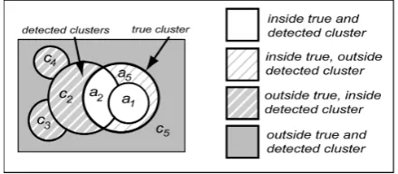
a,b,c,d notation used by Jacquez (2009), where areal units into one of four types (illustrated in Figure 1):

a) Inside both true and detected cluster(s) b) Inside true but outside detected cluster(s) c) Inside detected but outside true cluster(s) d) Outside both true and detected cluster(s)

A different, and slightly more succinct, subdivision method is used in papers introducing new versions of the SSS: Huang et al. (2007), Jung et al. (2007) and Jung et al. (2010). This is shown below, the relation-ship to the notation above given in brackets:

1_{The indicator function}_I_{evaluates to 1 when the expression}

[image:4.595.312.531.111.226.2]

fol-lowing in brackets evaluates true, 0 otherwise.

Figure 1: Example sub-regions

• The intersection of the true and detected cluster(s) (≡a)

• The true cluster(s) (≡a∪b)

• The detected cluster(s) (≡a∪c)

To use this kind of shorthand in the measures discussed in Section 2.4, one must first define scalar values to be associated with each sub-region2. This is simply the nu-merical integration of the data function f(s) across each

swithin the sub-region concerned. For any subregion

S, one express the its associated scalar value as:

Z

S

f(s∈S)ds

For example, consider Que et al. (2008). Here s are postal code area centroids and (amongst other things) the authors measure the count of areal units included in both true and detected clusters. Using Levels 1 to 3 of this framework, one would define the area of overlap be-tween true and detected clusters as a subregion (saya, for compatibility with Figure 1), and with this associate a value equal to the sum ofI(s∈ a) for all postal code centroids swithina. It is important to note that these sub-regions, and their associated scalar values, are de-pendant not only on the size and shape of the detected clusters, but on the significance threshold used to screen out unlikely clusters. For example, if one uses a typical significance threshold of 0.05, then ‘detected clusters’ means only those scan windows produced that have a p-value of≤0.05. This means that spatial accuracy, as

it is measured in the studies cited here, is dependent on the exact choice of significance threshold. Section 3 ex-plores this issue in more depth.

2_{Within this paper, sub-region notation such as}_a_,_b_,_c_,_d_{refers to}

(5)

The next section explains how the scalar values as-sociated with each sub-region are used to produce mea-sures of spatial accuracy.

2.4. Level 4: Performance measures

The first three levels of the framework give a modular way of considering location and data within each data set. The fourth level brings these together to produce actual values representing the spatial accuracy of a par-ticular detection method applied to a parpar-ticular data set. This is where the difference between studies is greatest. Read et al. (2009) and Savory et al. (2010) conducted benchmark studies where both the true and detected clusters have a clearly defined centre. Here the Eu-clidean distance between these centres provides a sin-gle, easily understandable measure of spatial accuracy. The advantage of a single measure is that it is straight-forward to rank different detection algorithms in terms of their spatial accuracy. Unfortunately, the presence of multiple true and detected clusters within one data set complicates this approach, except when the correspon-dence of each true and detected cluster is very obvious, as in Savory et al. (2010). Also, the distance measure approach does not take account of the size and shape of the true and detected clusters.

The use of two of more scalar measures provides more flexibility, especially where there may be multiple (possibly overlapping) true and detected clusters, any of which could be highly irregular in shape and varying in size. Rather than considering distance, these studies consider the amount of overlap between true and de-tected clusters, and the amount of overlap between the detected clusters and those parts of the study region out-side the true clusters. Examples of this approach can be found in Huang et al. (2007), Jacquez (2009), Jung et al. (2007), Jung et al. (2010), Neill (2009), Olson et al. (2006), and Que et al. (2008). All of the mea-sures used in these studies are, implicitly or explicitly, based upon scalar values calculated for each of the sub-regions shown in Figure 1. For example, consider the definitions ofspatial sensitivityandspatial positive

pre-dictive value(PPV) used in Huang et al. (2007), Jung

et al. (2007) and Jung et al. (2010). In an individual data set level, these can be expressed as=a/(a+b) and

=a/(a+c), respectively. To understand spatial accuracy measures calculated from the scalar values associated witha,b,candd, it is perhaps easiest to present them in the familiar 2×2 table used for calculating non-spatial measures (see Table 1).

The variety of measures used in various studies is shown in Table 2. Note that nomenclature varies from study to study, even when referring to what is essentially the

[image:5.595.346.494.109.139.2]

Inside true Outside true Inside detected a c Outside detected b d

Table 1: Adaption of standard 2×2 table for classifying the

sub-regions used in calculating spatial accuracy, after Jacquez (2009)

same thing. A particularly interesting measure is high-lighted by Neill (2009), who uses the terminology of information retrieval: recall= a/(a+b) andprecision

= a/(a+c). Recognising the value of having a single scalar measure of spatial accuracy when ranking diff er-ent methods, Neill uses an established method of com-bining these: the F-measure (van Rijsbergen, 1979), which is the harmonic mean of recall and precision. The only drawback is that the F-measure requires an as-sumption (implicit or explicit) about the relative weight-ing of recall and precision (Rennie, 2004). This issue is discussed further in Section 3.

2.5. Level 5: Aggregation

Each measure in Level 4 has a scalar variable as its output. This means that within each data set, spatial accuracy is represented by one or more (typically two) scalar values. However, benchmark testing involves manifold data sets, and one needs measures that rep-resent spatial accuracy at batch level, rather than indi-vidual data set level. The obvious choice is to take the arithmetic mean for each measure across all data sets in the batch. This is the approach taken by Huang et al. (2007), Jung et al. (2007), Jung et al. (2010), Neill (2009), Olson et al. (2006) and Que et al. (2008).

An alternative approach is taken by Waller et al. (2006), who take the mean across only those data sets where at least one cluster is detected with a p-value at or below the chosen significance threshold. This is a crucial choice which can make a significant difference to value of the aggregated measures, in difficult bench-marks tests where the power of the SSS is low, or if a very strict significance threshold is applied. Here only a small proportion of data sets may have detected clusters, and taking the mean across these data sets alone could give a volatile result. However, calculating the mean spatial accuracy across all data sets in a batch could be paradoxical: as one would then be including results from data sets where, statistically speaking, nothing has been detected (in which case the measures in Level 4 usually default to a certain value, e.g. zero).

(6)

• “Does this data set contain any true clusters, if so where are they?”

or two separate questions:

• “How certain am I this data set contains any true clusters?”

• “Where are any true clusters in this data set most likely to be?”

If one is certain it is the first, then clearly one only need consider data sets where a statically significant cluster is detected. Otherwise, one might consider all (or some) of the other data sets. Ironically, this is not a major is-sue in many existing studies as they generate data sets using models that result in true clusters that are not too difficult to detect.

Table 2 summarises all the studies mentioned in this section, outlined in terms of this framework. It can be seen that, due to the modular nature of the framework, a hybrid approach can be used to select aspects of spa-tial accuracy measurement from existing studies that are most suitable to the application concerned.

3. A unified measure of spatial accuracy

As discussed in Section 2.4, except in limited cases one needs at least two measures of spatial accuracy: one quantifying the amount of the true cluster that has been correctly detected, and one quantifying the amount of the study region outside the true cluster that has been incorrectly detected. However, if one wishes to rank different implementations of the SSS in terms of spa-tial accuracy, one needs to combine these functions into one scalar value. For the purposes of this discussion let us call thisdimension reduction. Neill (2009) achieved dimension reduction using the F-measure; however this implicitly requires an assumption about the weighting of the two dimensions being combined (in this case spa-tial precision and spaspa-tial recall). It would be advanta-geous to have a single measure of spatial accuracy that obviates the need to weight the dimensions concerned.

Furthermore, most of the measures of spatial accu-racy discussed in Section 2 are dependent on an arbi-trary choice of significance threshold. This is because each cluster detected by the SSS has an associated p-value, and when comparing detected and true clusters (e.g. when delineatingaandcin Figure 1) one would normally exclude detected clusters with unconvincingly high p-values. Thus, one must specify a significance threshold. One may then have a situation where one detection algorithm produces better spatial accuracy at

one threshold, and another algorithm performs better at another threshold. It would be advantageous to have a measure of spatial accuracy that covers all significance threshold levels simultaneously.

This section derives such a measure. The start-ing point is a two-alternative-forced-choice (hereafter 2AFC) test, similar to that used in the derivation of the

area under curve(AUC) measure3_{. AUC combines}

sen-sitivity and specificity to produce a single scalar value, which happens to equal the area under the correspond-ing receiver operatcorrespond-ing characteristic (ROC) curve. The AUC is equivalent to the probability that, when faced with one ‘true’ sample and one ‘false’ sample, the de-tection method under consideration can correctly iden-tify which is which. The use of this 2AFC obviates the need to make a decision about the weighting of sensi-tivity and specificity, or the significance threshold of the test.

The 2AFC test used in this section is a forced choice between two randomly selected locations, s1 and s2, both within the study region. Let s1 lie somewhere in-side the true cluster, and s2 somewhere outside4. Let

s1 be generated by a spatial Poisson process, such that any location inside the true clusters may be chosen with a probability density function proportional to the data function f(s) (see Section 2.2). Similar for s2. Let us define a measure called Ωrepresenting the probability that when one is presented blindly with these two loca-tions, and using only information provided by the SSS algorithm, one can correctly determine which iss1, and which is s2. It is important to note that one will never actually need to generate the locations s1 ands2, it is only the probability density functions of their potential locations that is of interest in calculatingΩ.

The definition ofΩgiven above is necessarily tech-nical for the purposes of the following proof. However, the idea of the probability of correctly choosing between two randomly selected locations, one inside the cluster and one outside, is straightforwardly intuitive. This is useful for non-technical readers of benchmark testing literature, who simply wish to know how well a detec-tion method is likely to perform when faced with real data.

To calculateΩ, it is necessary to define some addi-tional terms:

3_{Green and Swets (1966), revisited by Hanley and McNeil (1982)}

4_{This necessitates that there is a least one true cluster present in}

(7)

Study

Framework level (see text)

spatial data sub- performance aggregation support function regions measures

Huang et al. (2007) s=address f(s)= S=a,borc sensitivity Arith. mean Jung et al. (2007) s=census tract no. affected See

=a/(a+b)

over all individuals Figure1 data sets Jung et al. (2010) s=postal code ats generated

area PPV under same

=a/(a+c) model

Read et al. (2009) st=loci(centre) n/a n/a |st−sd|

of the true cluster sd=loci of most likely detected

cluster

Savory et al. (2010) st=loci(centre) n/a n/a Arith. mean of Arith. mean of each true cluster 1/|st−sd| and coeff. of sd=loci of each variance over all matching detected data set gen. under

cluster same model

Waller et al. (2006) s=census tract I(s∈S) S=a,borc Measure 1= Measure 1: where: I(a∩b,) Sum over all a=centre of Measure 2₌ data sets

true cluster I(a∩c,) wherea,

b₌centres of whereIis Measure 2: all sig. detected the indicator Sum over all

clusters function data sets c=all detected

clusters

Neill (2009) s=grid I(s∈S) S=a,borc recall Arith. mean

square See

=a/(a+b) over all Figure1 data sets

precision generated

=a/(a+c) under same model F-measure

=2a/(2a₊b₊c)

Jacquez (2009) s=county I(s∈S) S=a,b,cord power n/a

centroids See

=a/(a+b) Figure1

false neg.

=b/(a+b) false pos.

=c/(c+d) specificity

=d/(c₊d) detection acc.

=a/(a+c)

Que et al. (2008) s=postal I(s∈S) S=a,borc sensitivity Arith. mean

code area See

=a/(a+b)

over all Figure1 data sets

generated PPV under same

=a/(a+c)

model

Olson et al. (2006) s=address f(s)= S=a,borc Measure 1: orpostal code no. a_ffected See

=I(a≥b) area individuals Figure1

orcensus ats

tract Measure 2:

=c

Notes: I(∗) is the indicator function, whereI(∗)=1 if * true,I(∗)=0 otherwise PPV is positive predictive value

[image:7.595.116.482.109.709.2]

|st−sd|is the distance between pointsstandsd

(8)

• LetA(⊂R) be the locus of all true clusters inR

• LetAC=R−A, i.e. the locus of allRoutsideA

• Let{Z, α}represent a detected cluster, whereZ ⊆

Ris the locus of the detected cluster and theαis the p-value, i.e. probability5 _that _Z _{is a random} artefact.

• Let{α₁, α₂. . . α_X}be the set of all unique p-values associated with the detected clusters.

• Defineα0=0 andαX+1=1

• Let Zx be the union of all Z with associated p-value≤αx, where 1≤x≤X.

• DefineZ0=, andZX₊1=R

• Leta1=Z1∩A

• Letax=[Zx∩A−Six=−11ai] for 2≤x≤X

• Definea0=andaX₊1=A−SiX=1ai

• Letc1=Z1∪AC

• Letcx=[Zx∪AC−Six=−11ci] for 2≤x≤X

• Definec0=andcX₊1=AC−SXi=1ci

Put more intuitively:Z_xrepresents an amalgamation of the SSS output for each unique p-value, where all de-tected clusters with a p-value equal to or less thanαx are merged. Alsoa1 ∪c1 represents the locus of the most likely detected clusters, whilstax∪cxrepresents the locus of thexth_{most likely detected cluster,}

exclud-ing locations included in the loci of more likely clusters. Note thataX+1is equivalent tobin Figure 1, withcX+1 equivalent tod(this simplifies the expression forΩ). An example of this new spatial set notation is shown in Fig-ure 2; note thata3,a4andc1all happen to be null in the example illustrated.

As described in Section 2, one can numerically integrate the data function across each sub-region

a1. . .aX+1 andc1. . .cX+1, to obtain scalar values rep-resenting the probability of s1 ands2 being located in each, respectively. Using these values, one can calcu-lateΩusing the following formula:

Ω =

PX+1 y=1

h_P_y−1 k=0ak+

1 2 ay

i

·cy

PX+1

k=0ak·PXk=+01ck

(1)

5_{For all but the most likely cluster, this probability is known to be}

[image:8.595.310.530.111.207.2]

slightly conservative (Kulldorff, 1997).

Figure 2: Example of subdivisions used in definingΩ

This gives a value from 0 to 1, withΩ =1 representing perfect spatial accuracy, where all detected clusters lie within the true clusters, and all true clusters lie within the detected clusters. As with the AUC measure, if one obtainsΩ =0, i.e. perfect spatial inaccuracy, one could simply invert the detected clusters to achieve Ω = 1. Hence for practical purposes,Ω =0.5 is the worst case. This means the detection system has provided no useful information in distinguishing which location is s1 and which s2, and the probability of guessing correctly is the same as if one were tossing a coin. The proof of the formula is as follows.

Proof. First, letiandjbe the indices of the most signif-icantZto contains1ands2(respectively), with 1 being the most significant andXbeing the least. If eithers1or

s2 fall outside ofZX, letior j(respectively)=X+1. Therefore:

i=

(

i: s1∈ Zi,s1<Zi+1 if 1≤i≤X

i=X+1 otherwise

j= (

j:s2∈ Zj,s2<Zj+1 if 1≤ j≤X

j=X+1 otherwise

With regard to the 2AFC, if one is presented blindly with locations s1 ands2, and one’s decision is only in-formed by the SSS output, then there are just three pos-sibilities:

• P1: ifi< j, one will answer correctly with proba-bility 1

• P2: ifi> j, one will answer incorrectly with prob-ability 1

(9)

Usingρto denote the probability, thenΩby definition equals:

Ω =ρ(P1)+0.5ρ(P3)

=ρ(i< j)+0.5ρ(i= j)

=ρ(i<y| j=y)+0.5ρ(i=y| j=y)

Whereyis some integer. Taking marginal probabilities over possible values ofygives us:

Ω =

X+1

X

y=1

ρ(i<y)·ρ(j=y)

+0.5 X+1

X

y=1

ρ(i=y)·ρ(j=y)

=

X+1

X

y=1

ρ(_i<_y₎+0.5ρ(_i=_y₎_·ρ(_j=_y₎

Each probability can be expressed as follows:

ρ(i<y)=

Py−1

k=0ρ(s1∈ak)

PX+1

k=0 ρ(s1∈ak)

(2)

ρ(i=y)= ρ(s1∈ay)

PX+1

k=0 ρ(s1∈ak)

(3)

ρ(j=y)= ρ(s2∈cy)

PX+1

k=0 ρ(s2∈ck)

(4)

Because Ω is being defined in conjunction with the framework described in Section 2, we can draw upon the assumption made in Level 2 (see Section 2.2). This states that the data functionf(s) must be proportional to the probability density function ofs, whensis the out-put of a spatial Poisson process. Ass1ands2 are ran-domly generated under such a process, one can write:

ρ(s1∈ak)∝

Z

ak

f(s) ds

ρ(s2∈ck)∝

Z

ck

f(s) ds

When we are discussing a1. . .aX+1 and c1. . .cX+1 in terms of their scalar values, we can write the above ex-pressions simply as:

ρ(s1∈ak)∝ak ρ(s2∈ck)∝ck

Now to obtain exact values for these probabilities, one would divideakby (a1+a2+· · ·+aX) andckby (c1+

c2+· · ·+cX). However, as these denominators are the

same for allakandckrespectively, we can discard them when inserting the above values into Expressions 2, 3 and 4, which then become:

ρ(i<y)=

Py−1

k=0ak

PX+1 k₌0 ak

ρ(i=y)= ay

PX+1 k=0 ak

ρ(j=y)= cy

PX+1 k=0ck

Now inserting these into our previous expression forΩ gives Expression 1:

Ω =

PX+1 y=1

h_P_y₋₁

k=0ak+ 1 2 ay

i

·cy

PX+1

k=0 ak·PkX=+01ck

4. Example application

This section provides an example application of the framework presented in Section 2 and the Ωmeasure presented in Section 3. The number of candidate de-tected clusters produced by implementations of the SSS can be considerable. To aid users, SaTScanTM_provides

(10)

F1: No geographical overlap

F2: No cluster centres in other clusters

F3: No cluster centres in more likely clusters

F4: No cluster centres in less likely clusters

F5: No pairs of centres both in each others clusters

F6: No restrictions, i.e. most likely cluster for eachs

Here we briefly present the results of a benchmark study of filtering options, measuring spatial sensitivity and PPV (as defined in the sub-regions and performance measure columns of table 2), andΩas defined in Sec-tion 3. The benchmark data sets used are similar to those in Read et al. (2009), where full details of the generation procedure is given. Each data set is a randomised distri-bution of 100 cases of a hypothetical disease, and 200 controls. Four batches were used; two generated using an homogeneous background density (CSR for short6); two using an inhomogeneous background density pro-portional to the 2001 population of the Trent region of the UK (TRENT for short). The background density is (effectively) the underlying spatial distribution of con-trols, i.e. the probability of a control occurring at a par-ticular point is proportional to the background density at that point. E.g. in CSR data sets a control is equally likely to occur at any point with the study space.

The underlying distribution of cases follows that of controls, aside from the injection of one (×1TC) or three (×3TC) true clusters, i.e. one or three localised multi-plicative increases in risk. These injections are Gaussian in shape (i.e. the increase is highest at the centre then tails offsmoothly), isotropic, and uniformly randomly located7_{. The risk multiplier at the centre of each} in-jection is termed the maximum relative risk(hereafter MRR). All MRR values were set to 15; which gave> 50% power in all batches for a standard 5% false alarm rate. Although a potential limitation of the study, this use of consistent sizes and shape of anomaly consider-ably reduces the number of different batches required, making this preliminary study feasible. The reference codes used in this study are given in Table 3.

For each data set in each batch, SaTScanTM _{was run}

six times on each data set, once for each choice of out-put filter (F1 - F6). Four batches of 1000 data sets, and

6_{CSR stands for “complete spatial randomness”, referring to the}

spatial distribution of controls in these data sets.

7_{With the exception of an exclusion area close to the border to}

avoid the need to consider edge effects.

Batch code Description

CSR×1TC

1000 data sets, each with:

one true cluster, MRR=15 background density=CSR

CSR×3TC

three true clusters, MRR=15 background density₌CSR

TRENT×1TC

one true cluster, MRR=15 background density∝pop. of Trent, UK

TRENT×3TC

[image:10.595.328.509.109.220.2]

three true clusters, MRR₌15 background density∝pop. of Trent, UK

Table 3: Description of the four batches tested

six filters, gives 24,000 sets of results in total. A com-bination of Linux scripts and a MATLABTM _program

was used to extract true and detected cluster information from each, and calculate spatial sensitivity and PPV, and

Ω.

Following the framework presented in Section 2, in similar layout to Table 2, the measures are shown in Ta-ble 4. Note the use a data function (Level 2) based on λ(s)×rr(s) rather than the count of events or areal units. λ(s) is the background event rate at s, andrr(s) is the multiplicative relative risk atsdue to any true cluster lo-cated nearby; ifsis unaffected by true clustersrr(s)=1. This is more representative than the count of areal units, as it takes account of background population. It should also have lower variance than measures based on counts of events, which are inevitably subject to more random variation than the underlying risk value. For Level 5, two types of aggregation method were used. As Ωis intended to be independent of significance threshold, it is here averaged across all data sets. As sensitivity and PPV are linked to a particular significance thresh-old (here chosen as 0.05), they were averaged across only those data sets where the most likely cluster had a p-value of≤0.05.

The results for each measure, for each batch and filter combination, for both scans, are shown in Table 5. As MeanΩcan be used for ranking the different filters in terms of spatial accuracy, a 95% confidence interval is included (shown as a±in brackets, based on the stan-dard error). It can be seen that, in terms of all three measures, filter performance falls into two loose group-ings; F1, F2 and F4 tend to have lowerΩ, lower sensitiv-ity, and higher PPV; F3, F5 and F6 tend to have higher

(11)

Framework level (see text) spatial data sub- performance

aggregation support function regions measures

s=point

f(s)=λ(s)×rr(s) _{

ai},{ci} _Ω Arith. mean over

where: all data sets

λ(s)₌background event

rate ats a,b,c,d sensitivity Arith. mean over all (at sig. =a/(a+b) data sets with at rr(s)=relative risk threshold 0.05) PPV least one detected

atsattributable to =a/(a+c) cluster at sig. true clusters threshold 0.05 (=1 outside clusters)

[image:11.595.151.442.110.242.2]

Notes: For examples of{ai}and{ci}see Figure 2. PPV is positive predictive value.

Table 4: Measures used in Section 4, in context of the framework presented in Section 2.

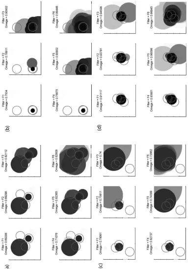
Figures 3a-d provide some explanation of this. Each figure represents the results of the six filter choices on a randomly selected data set from batch CSR×3TC. For each filter choice, the six charts within contain out-lined and solid circles, with an Ω value above. The outlined circles delineate A in three (sometimes over-lapping) parts, each being the outer limit8 _{of a} Gaus-sian shaped true cluster. The solid circles represent the detected clusters passed by the filter, shaded relatively from dark (low p-values) to light (high p-values); the shading is relative within each chart becauseΩis only concerned with the relative p-values of different circles. Hence a shade in one chart may represent a different p-value to the same shade in a different chart. Note that more likely detected clusters overlap less likely ones, as per Figure 2. Note also that asλ(s) is uniform in CSR datasets, Ω (and sensitivity) rewards correct detection of the centre of each true cluster much more than the periphery. Due to varyingλ(s), charts for TRENT data sets are harder to interpret and are not presented here.

It can be seen in Figures3a-d that filters F1, F2 and F4 generally pass fewer (and smaller) detected clusters than F3, F5 and F6. This explains the contrast between spatial sensitivity and PPV in the two groupings. On no occasion are the true clusters correctly delineated, but this is hardly surprising given that the SSS has only 300 points locations in total for each data set. As can be seen in Table 4, F6 performed unquestionably better in each batch,Ωwise, with the exception of TRENT×3TC where it is highest, but by a much smaller margin. This is counter intuitive, as F6 is the null option, i.e. no fil-tering. However, recall thatΩis the probability that one can correctly decide which of two randomly generated points lies inside the true clusters, based only on

infor-8_{This is the loci of}_s_where_rr₍_s₎_>₀_._{00001. This limit is}

arbi-trary, but varying this value by several decimal places either way has negligible effect on any of the measures.

mation provided by the detected clusters. If one views the unfiltered SSS output as a probability map of where the true clusters are more likely to be, rather than as a list of individually detected clusters, then it is hardly surprising that it provides the best source of information on spatial accuracy. However, if a more succinct list of detected clusters is desirable, then one should apply fil-ters F1, F2 or F4, with filter F2 (no cluster centres in other clusters) performing best in terms ofΩin all four batches used in this study.

MeanΩ Mean over all data sets sig. at 0.05 over all data sets sensitivity PPV

CSR

×

1TC

F1 0.7364 (±0.0037) 0.838245 0.596085 F2 0.7659(±0.0040) 0.841861 0.591564 F3 0.8684 (±0.0044) 0.877693 0.46603 F4 0.7612 (±0.0039) 0.850334 0.594105 F5 0.8725 (±0.0044) 0.882901 0.466492 F6 0.8962 (±0.0044) 0.920411 0.380853

CSR

×

3TC

F1 0.7402 (±0.0028) 0.537794 0.572392 F2 0.7704 (±0.0031) 0.545679 0.562416 F3 0.8466 (±0.0030) 0.637829 0.388202 F4 0.7654 (±0.0030) 0.548487 0.565982 F5 0.8518 (±0.0029) 0.641853 0.387308 F6 0.8631 (±0.0030) 0.681826 0.31248

TRENT

×

1TC

F1 0.7315 (±0.0038 0.858498 0.759631 F2 0.7582 (±0.0041) 0.876176 0.710421 F3 0.8746 (±0.0045) 0.947331 0.345964 F4 0.7519 (±0.0040) 0.878359 0.73161 F5 0.8779 (±0.0044) 0.948619 0.34458 F6 0.8874 (±0.0045) 0.963441 0.264817

TRENT

×

3TC

[image:11.595.311.528.411.632.2]

F1 0.7124 (±0.0033) 0.695842 0.786179 F2 0.7455 (±0.0036) 0.719602 0.735298 F3 0.8430 (±0.0031) 0.841569 0.396941 F4 0.7354 (±0.0035) 0.718791 0.76095 F5 0.8477 (±0.0031) 0.84665 0.39312 F6 0.8486 (±0.0032) 0.874754 0.30667

Table 5: Spatial accuracy results for the four batches, with output filters F1 to F6 applied.

5. Discussion and future directions

(12)

[image:12.595.102.486.132.682.2]

(13)

a universal definition of spatial accuracy for the SSS. Given the range of different measures, suited to diff er-ent studies and different kinds of data, this seems un-likely. However a framework, such as the one presented here, may at least provide a means of comparing dif-ferent methods, and help to avoid “reinvention of the wheel”. The main limiting factor of the framework is that it is currently only suitable for measures of spatial, not spatio-temporal, accuracy. In studies where time can be considered as an extra spatial dimension, e.g. a one-off retrospective study, then the framework should be applicable. In contrast, with the detection of emerging clusters the direction and currency of time makes it dif-ferent to space9. It may be feasible to extend this frame-work to cover spatio-temporal accuracy, and this could be a direction for future research.

TheΩmeasure presented in Section 3 provides a so-lution to the problem of arbitrarily specifying a signif-icance threshold and the relative weighting of existing measures such as spatial sensitivity and PPV. As it fits within Levels 3 and 4 of the framework described in Section 2,Ωcan be used with any combination of spa-tial support and data, not just the case/control data used in the example study. The chief drawback is that, for most existing studies, implementingΩrequires writing additional code and re-examining the SSS output files. If one is happy to specify a significance threshold, then easier to calculate (if somewhat cruder) single measures are available, based upon a similar 2AFC toΩ. Details available from the corresponding author.

Although limited in scope, the preliminary study of SaTScanTM_{filter options presented in Section 4 is, so far}

as we are aware, the first of its kind to be published. Despite being part of a particular software package, in some form or other these filters would be a natural part of any SSS implementation. The observation thatΩ ap-pears to be optimised by not applying a filter does not diminish their usefulness, but it does suggest that an-other means of presenting SSS output, beyond a simple list of detected clusters, could be beneficial. Studies in visualising SSS output already exist (e.g. Boscoe et al. (2003) Chen et al. (2008)), and one future research di-rection could be to investigate the spatial accuracy of different visualisation techniques, however that might be defined. We hope the material contained in this pa-per is of interest to those in the research community and welcome feedback.

9_{For the interested reader, an approach to measuring}

spatio-temporal accuracy (which treats time as something fundamentally dif-ferent from space) is given in Fricker Jr. (2010)

6. Acknowledgements

We thank the Medical Research Council for funding Simon Read, the principal author, researcher and pro-grammer on this project.

References

Boscoe FP, McLaughlin C, Schymura MJ and Kielb CL. Visualization of the spatial scan statistic using nested circles. Health & Place 2003;9(3):273-277.

Chen J, Roth R, Naito A, Lengerich E and MacEachren A. Geovisual analytics to enhance spatial scan statistic interpretation: an analysis of U.S. cervical cancer mortality. Int J Health Geogr 2008;7(1):57.

Fricker Jr. RD. Rejoinder: some methodological

is-sues in biosurveillance. Retrieved July 16th, 2010,

from: http://faculty.nps.edu/rdfricke/docs/

Rejoinder%20-%20Issues%20in%20Biosurveillance.pdf. Monterey CA: Navel Postgraduate School; 2010.

Green DM, Swets JA. Signal detection theory and psychophysics. New York: Wiley; 1966.

Hanley JA, McNeil BJ. The meaning and use of the area under a re-ceiver operating characteristic curve. Radiology 1982;143(1):29-36.

Huang L, KulldorffM, Gregorio D. A spatial scan statistic for survival

Data. Biometrics 2007;63(1):109-118.

Jacquez GM. Cluster morphology analysis. Spat Spattemporal Epi-demiol 2009;1(1):19-29.

Jung I, KulldorffM, Klassen AC. A spatial scan statistic for ordinal

data. Stat Med 2007;26(7):1594-1607.

Jung I, KulldorffM, Richard OJ. A spatial scan statistic for

multino-mial data. Stat Med 2010;29(18):1910-1918.

KulldorffM, Nagarwalla N. Spatial disease clusters, detection and

in-ference. Statistics in Medicine 1995;14:799-810.

KulldorffM. A spatial scan statistic. Commun Stat Theory Methods

1997;26(6):1481-1496.

Kulldorff, M. SaTScan user guide for version 8.0. Cambridge MA:

Harvard; 2009.

Neill DB. Expectation-based scan statistics for monitoring spatial time series data. Int J Forecast 2009;25(3):498-517.

Olson KL, Grannis SJ, Mandl KD. Privacy protection versus cluster detection in spatial epidemiology. Am J Public Health 2006;96(11):2002-2008.

Que J, Tsui F-C, Espino J. A Z-Score based multi-level spatial clus-tering algorithm for the detection of disease outbreaks. Lect Notes Comput Sci 2008;5354:108-118.

Read S, Bath, PA, Willett P, Maheswaran R. A spatial accuracy

assess-ment of an alternative circular scan method for Kulldorff’s spatial

scan statistic. In: Fairbairn D, editor. Proceedings of the GIS Re-search UK 17th Annual Conference, Durham University, 1st - 3rd April 2009. Durham: Durham University; 2009. p. 57-62. Rennie JDM. Derivation of the F-Measure. retrieved July 16th, 2010,

from: http://www.ai.mit.edu/people/jrennie/writing/fmeasure.pdf. Cambridge MA: MIT; 2004.

Savory D, Cox K, Emch M, Alemi F, Pattie D. Enhancing spatial de-tection accuracy for syndromic surveillance with street level inci-dence data. Int J Health Geogr 2010;9(1):1.

van Rijsbergen CJ. Information retrieval. London: Butterworths; 1979.