Macroevolutionary consequences of profound climate change on niche evolution in 1
marine molluscs over the past three million years 2
3
Saupe, E.E.1*; Hendricks, J.R.2; Portell, R.W.3; Dowsett, H.J.4; Haywood, A.5; Hunter, 4
S.J.6; Lieberman, B.S.7 5
6
1Biodiversity Institute and Department of Geology, University of Kansas, 1475 7
Jayhawk Boulevard, Room 120 Lindley Hall, Lawrence, KS 66045 8
9
2Department of Geology, San José State University, Duncan Hall 321, San José, CA 10
95192 and Paleontological Research Institution, 1259 Trumansburg Road, Ithaca, NY 11
14850 12
13
3Division of Invertebrate Paleontology, Florida Museum of Natural History, 14
University of Florida, 1659 Museum Road, PO Box 117800, Gainesville, FL 32611 15
16
4U.S. Geological Survey, 926A National Center, Reston, VA 20192 17
18
5School of Earth and Environment, University of Leeds, Leeds, LS2 9JT, United 19
Kingdom 20
21
6Sellwood Group for Palaeo-Climatology, University of Leeds, Room 9.127 Earth and 22
Environment Building, School of Earth and Environment, West Yorkshire, LS2 9JT, 23
United Kingdom 24
25
7Biodiversity Institute and Department of Ecology & Evolutionary Biology, University 26
of Kansas, 1345 Jayhawk Boulevard, Dyche Hall, Lawrence, KS 66045 27
28
*Corresponding author: Erin E. Saupe; [email protected] 29
30
Summary 31
In order to predict the fate of biodiversity in a rapidly changing world, we must first 32
understand how species adapt to new environmental conditions. The long-term 33
evolutionary dynamics of species’ physiological tolerances to differing climatic regimes 34
remains obscure. Here, we unite palaeontological and neontological data to analyse 35
whether species’ environmental tolerances remain stable across three million years of 36
profound climatic changes using ten phylogenetically, ecologically, and developmentally 37
diverse mollusc species from the Atlantic and Gulf Coastal Plains, USA. We additionally 38
investigate whether these species’ upper and lower thermal tolerances are constrained 39
across this interval. We find that these species’ environmental preferences are stable 40
across the duration of their lifetimes, even when faced with significant environmental 41
perturbations. The results suggest that species will respond to current and future warming 42
by altering distributions to track suitable habitat, or, if the pace of change is too rapid, by 43
going extinct. Our findings also support methods that project species’ present-day 44
46 47
Keywords Atlantic Coastal Plain | conservation palaeobiology | fundamental niche | 48
macroevolution | mid-Pliocene Warm Period | Mollusca 49
50
1. Introduction 51
Earth’s climate is rapidly changing, altering all facets of our planet at an 52
unprecedented rate, from the biosphere, to the hydrosphere, to the atmosphere. Given 53
these changes, debate exists as to whether species can adapt their physiological tolerances, 54
or niches, to altered environmental conditions [1-4]. Determining whether species’ niches 55
evolve or remain stable in the face of environmental change is important for 56
implementing proper conservation measures, mitigating threats posed to biodiversity [5-57
7], and for shedding light on macroevolutionary dynamics [8-11]. 58
Here, we unite palaeontological and neontological data [12] to test niche stability 59
across three million years of environmental changes using ten phylogenetically, 60
ecologically, and developmentally diverse bivalve and gastropod species from the 61
Atlantic and Gulf Coastal Plains, USA, and surrounding region (electronic supplementary 62
material, table S1). Species’ niches were quantified using ecological niche modelling [13] 63
for three time periods from the Pliocene—recent: the mid-Pliocene Warm Period 64
(mPWP; ~3.264–3.025 Ma); the Eemian Last Interglacial (LIG; ~130–123 Ka); and the 65
present-day interval (PI). We test whether these species’ niches changed across both long 66
(Pliocene to Eemian; millions of years) and short (Eemian to present-day; thousands of 67
years) time scales. We additionally investigate whether these species’ upper and lower 68
thermal tolerances changed across millions of years. Recent research suggests that 69
tolerances to heat are largely conserved within terrestrial species, but that tolerances to 70
where ectotherms are limited by both cold and warm conditions due to decreased aerobic 72
capacity [15]. This study is the first to incorporate both modern and fossil data across 73
millions of years to understand ecological and evolutionary responses of species to 74
changes in their environment, though see [16-18] for analyses in deep time. 75
Theoretical [19, 20] and empirical studies have both supported [21, 22] and 76
questioned [16, 23, 24] niche stability. The debate has even continued at the genetic level, 77
where recent research indicates that genetic reshuffling in Drosophila species can occur 78
in response to climate change [25, 26]. Whether these genetic changes translate into 79
evolution of actual physiological tolerances, however, remains unclear. The context in 80
which niche evolution is considered is important with respect to whether change occurred 81
in actual physiological tolerances (i.e., the fundamental niche; FN), or whether change 82
occurred because of differences in resource utilization or underlying environmental 83
structure (i.e., changes in the realized niche; RN). Studies may incorrectly indicate niche 84
evolution if the environmental conditions that are available to a species are not taken into 85
account [4, 27, 28]. 86
The aforementioned studies have contributed much to our understanding of how 87
species’ environmental tolerances evolve, but questions about the relative dominance of 88
niche evolution versus stability remain, particularly since most studies lack a temporal 89
component that would allow for analysis of change across the entire duration of a 90
species’ lifetime, which may span millions of years [8]. 91
The region encompassing and surrounding the Atlantic and Gulf Coastal Plains is 92
ideal for elucidating the coevolution of species’ niches and the environment. Not only has 93
it experienced profound environmental changes associated with the closure of the Central 94
been linked to patterns of extinction, species turnover, and ecological change [30, 31]. 96
The mPWP is considered a climatic analogue for conditions expected at the end of this 97
century and can contribute information on how target species may fare under future 98
climate scenarios [32]. Results such as those presented here are vital for proper mitigation 99
of the risks posed by current and future climate changes to Earth’s biodiversity [7, 33]. 100
101
2. Materials and methods 102
In order to test for within-lineage niche stability, we used ecological niche 103
modelling (ENM), a correlative process whereby known occurrences of species are 104
associated with environmental parameters to characterize a species’ environmental 105
requirements [13]. Models of species’ abiotic niche parameters were constructed for each 106
of three temporal intervals—the mPWP, LIG, and PI—using taxon occurrence data and 107
environmental parameters unique to each time slice. The resulting niche estimates were 108
compared through time to statistically assess similarity using both environmental and 109
geographic approaches [28, 34, 35]. In both approaches, an observed similarity metric is 110
computed and compared to a simulated null distribution. Details of our methodology are 111
outlined below. 112
113
(a) Taxa 114
We selected ten species that occur in both the modern and fossil (from ~3.1 Ma to 115
recent) records of the Atlantic and Gulf Coastal Plains, USA, and surrounding region 116
(Table 1). Species were chosen because they have diverse phylogenetic positions, varied 117
ecological habits and larval developmental modes, and abundant distributional data 118
We used morphological criteria to identify target species, as each taxon is readily 120
diagnosable. All evidence suggests that these lineages represent species that have distinct 121
evolutionary trajectories, a supposition supported by the fact that many invertebrate 122
species have durations greater than three million years [8]. Consequently, we studied 123
within-lineage rather than across-lineage niche evolution, although see the Discussion 124
section for potential caveats. 125
126
(b) Distributional data 127
Present day. Presence-only distributional data were derived from [36] (electronic 128
supplementary material, table S1 and figures S1-3). Only records with spatial uncertainty 129
<15 km were retained, ensuring that they were matched correctly with corresponding 130
environmental data of a coarser spatial resolution (i.e., 1.25 x 1.25°) [37]. We 131
subsampled distributional data to leave one record per environmental pixel to account for 132
sampling biases in R.15.2 (R Core Team, 2012), which resulted in 20–58 unique 133
occurrences per species (electronic supplementary material, table S1). This process did 134
not affect the resultant overall distribution of the species, but rather prevented certain 135
localities with multiple records from being unduly weighted in the niche modelling 136
analyses [38, 39]. 137
Fossil. We considered fossil distributional data from mPWP (~3.264–3.025 Ma) 138
and LIG (~130–123 Ka) strata of the Atlantic and Gulf Coastal Plains, USA, and 139
surrounding region. To ensure distributional data were derived from geologic units of 140
similar ages to our periods of interest, we generated a stratigraphic database for all 141
Pliocene–recent geologic units of the Atlantic Coastal Plain (electronic supplementary 142
survey and use of various stratigraphic databases, resulting in ten viable formations for 144
the Pliocene and 16 for the LIG. The formations from which occurrence data were 145
derived are documented in dataset S1. 146
Distributional records were obtained from onsite investigations of collections to 147
ensure proper species identification, including the Florida Museum of Natural History, 148
Paleontological Research Institution, Virginia Museum of Natural History, Academy of 149
Natural Sciences of Drexel University, and Yale Peabody Museum. As with present-day 150
distributional data, we subsampled fossil distributional data to leave one record per 151
environmental pixel, resulting in six to 16 unique occurrences per species (electronic 152
supplementary material, table S1). At least six spatially-explicit distributional records 153
were used for model calibration for any given species/time period; studies have shown 154
this number to be statistically robust for extant species [40, 41]. 155
156
(c) Environmental data 157
Environmental data were derived from the coupled atmosphere-ocean HadCM3 158
global climate model (GCM) [42, 43] for three time slices: mPWP (~3.264–3.025 Ma), 159
LIG (~130–123 Ka), and PI (considering the pre-industrial interval from ~1850–1890). 160
Ideally, we would use an ensemble-modelling approach that considered multiple GCMs 161
[44]; however, model output for the LIG was available to us only from HadCM3 and 162
consisted of variations of temperature and salinity parameters. This GCM has been 163
successfully used in a variety of Quaternary and pre-Quaternary modelling studies [45-164
47]. Boundary conditions for the LIG were from [46] and [48]. Here, atmospheric gas 165
concentrations were derived from ice core records [49-51], and orbital parameters were 166
dataset [53], and the pre-industrial experiment was equivalent to [54]. All GCM 168
experiments were run for 500 model years, and environmental parameters were averaged 169
from the final 30 years of each experiment at 1.25 x 1.25° resolution (~140 x 140 km at 170
the equator). Where ocean data were unavailable (i.e., sites presenting macrofossil data, 171
but where the GCM indicated land), we used an inverse-distance weighted algorithm to 172
extrapolate model data. 173
Modelled monthly salinity and temperature outputs were converted to maximum, 174
minimum, and average yearly coverages for both surface and bottom conditions using 175
ArcGIS. From these 12 coverages, we eliminated variables that significantly co-varied 176
(assessed using the ‘cor’ function in R.15.2; R Core Team, 2012). Ultimately, two bottom 177
variables (yearly average salinity and temperature) and four surface variables (maximum 178
and minimum salinity, and maximum and minimum temperature) were retained. These 179
six variables were preserved because they did not significantly co-vary and are deemed 180
biologically important for marine ectotherms [55-57]. 181
182
(d) Modelling algorithm 183
To approximate niche parameters for these species, we generated ENMs using 184
Maxent v.3.3.3 [58] (figure 1 and electronic supplementary material, figures S4-5). 185
Maxent finds suitable environmental combinations for species under a null expectation 186
that suitability is proportional to availability. Thus, Maxent minimized the relative 187
entropy of observed environments relative to those in the background [59]. We enabled 188
only quadratic features to simulate realistic bell-shaped response curves that are known 189
from physiological experiments of plants and animals [60-62]. We calibrated models 190
latitude (figure 1). We sought the union of the area sampled by researchers and most 192
likely accessible to the species across spatial and temporal dimensions [13, 63, 64]. We 193
used all spatially-explicit data points for each species/time slice, running 100 bootstrap 194
replicates with a ten per cent random test percentage. The mean value of the suitability 195
grids was used to threshold to binary predictions [65, 66]. 196
To correct for potential biases in fossil distributional data, we implemented what 197
is called a ‘bias file’ within Maxent for past modelling [67]. The bias file describes the 198
probability that an area was sampled; thus, regions with rock outcrop (i.e., areas where 199
species may actually be sampled) were weighted twice as heavily as regions without rock 200
outcrop. Maxent will then factor out this bias during the modelling process (see [67] for 201
details). This method essentially accounts for incomplete knowledge of species’ 202
distributions sensu [68]. 203
Although characterizing the entirety of a species’ FN is often difficult without 204
mechanistic studies [14], we study close approximations here, given that recent 205
biophysical approaches have determined that FNs can be represented by limited sets of 206
parameters such as temperature [69, 70]. This is particularly true for marine ectotherms, 207
which have been shown to closely match range limits within their thermal tolerances [15]. 208
That being said, our estimates may reflect some quantity between the RN and the FN, 209
since our niche parameters are ultimately derived from the areas occupied by a species 210
[13, 14, 27]. 211
212
(e) Model verification 213
Two model validation methods were used, depending on the prevalence of 214
slices with <25 points, we assessed statistical significance using a jackknife procedure 216
under a least training presence threshold [41]. This method, however, may produce over-217
optimistic estimates of predictive power for sample sizes >25, and these species/time 218
slices were tested using partial Receiver Operating Characteristic analyses [71]. 219
220
(f) Niche comparisons 221
Characterizations of species’ niches were compared through time using two 222
statistical approaches: a kernel smoothing script [28] and ENMTools [35]. Both 223
frameworks use randomization tests to compare observed similarity to that expected 224
under a null hypothesis. The null is rejected if models are more or less similar than 225
expected by chance, based on the environment within the geographical regions of interest. 226
Similarity is quantified using Schoener’s D [72], with values ranging from 0 to 1, or more 227
to less similar, respectively. 228
For each of the ten species, we compared observed niches across the three 229
different time periods (mPWP, LIG, and PI). Comparisons were made in two directions 230
[28, 35]; e.g., comparing the mPWP to the LIG, and the LIG to the mPWP, since it is 231
possible for two niches to be more similar than expected based on the environment 232
available for one time slice, but less similar than expected based on the environment 233
available for the other. If the observed value fell outside the null distribution to the high 234
end, niches were more similar than expected by chance, whereas if the observed value 235
fell outside the null distribution to the lower end, niches were more different than 236
expected by chance. Observed values that fell within the null distribution did not allow 237
for discrimination of similarity or differences based on the environment available to the 238
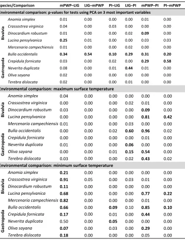
environmental variables; (2) a PCA applied to the three most important environmental 240
variables; (3) raw average bottom temperature and maximum surface temperature in two-241
dimensional environmental space; (4) maximum surface temperature only; (5) minimum 242
surface temperature only; and (6) ENMTools on projections of ecological niche models. 243
The first five sets of tests compare niches in environmental space, with the first three 244
multi-dimensional in nature, whereas the sixth compares niches in geographic space. 245
Each of these tests resulted in 60 comparisons (i.e., 10 species x three time slices x two 246
directions), for a total of 360. Details of the comparisons are provided below. 247
Environmental comparisons. We calculated metrics of niche overlap in gridded 248
environmental space using the methodology of [28]. Here, ordination techniques [73] 249
allow for direct comparison of species-environment relationships in environmental space 250
[27]. Observed densities for each region are corrected in light of the availability of 251
environmental space using kernel density functions (table 1 and electronic supplementary 252
material, table S3 and dataset S2). Niche overlap is measured along gradients of a 253
multivariate analysis, and statistical significance is assessed using the framework 254
described above. 255
We tested for similarity using a principal component analysis (PCA) (1) applied 256
to all six environmental parameters, and (2) when niche dimensionality was reduced to 257
three variables, including surface coverages for maximum salinity, maximum 258
temperature, and minimum temperature. These variables were retained because they 259
explained the most variance in the dataset [57, 74, 75]. Analyses performed with this 260
reduced set of variables are potentially more informative, as over-parameterization can 261
constrict niche estimates and lead to approximations closer to the RN [13]. PCA analyses 262
used both the PCA-occ and PCA-env functions; the former calibrates the PCA based only 264
on the distributional data, whereas the latter uses data from the entire environmental 265
space of the two study systems. The results were equivalent, and thus we present only 266
those from PCA-env. A bin size of 100 was used to characterize the environment, 267
running 1,000 replicates for similarity tests. Since prevalence of distributional data varies 268
through time, we generated input data from ENMs outside of the framework of [28], 269
subsampling one point per pixel in binary predictions such that comparisons were 270
unbiased with regard to the quantity of input data. Doing so ensures that we capture all of 271
the environments that a species finds suitable, rather than the portion that happened to be 272
occupied most frequently. 273
We also tested similarity in raw variables (table 1 and electronic supplementary 274
material, table S3 and dataset S2). We used the script of [28] to analyse each of the six 275
variables individually, and we modified the script to compare raw variables in two 276
dimensions, while still accounting for differences in availability of environments in a 277
given time period. We were interested in testing for evolution in overall temperature 278
parameters, and thus we assessed similarity using average bottom temperature and 279
maximum surface temperature. 280
Geographic projections. In addition to the comparisons made entirely in 281
environmental space, we used ENMTools [35] to compare the geographic projections of 282
niches. Null distributions consisted of 100 random models generated within Maxent, with 283
model parameters drawn from and constrained by the study system. To ensure accurate 284
response curves when projecting, we disabled clamping and enabled extrapolation within 285
Maxent [76]. 286
3. Results 288
Model verification exercises suggest that models of species’ niches are 289
statistically significant for each time slice (P<0.05; see electronic supplementary material, 290
table S2). The niche model depictions are shown in figure 1 and electronic supplementary 291
material, figures S4-5. 292
Together, the suite of niche comparisons (360 in total) indicates these species’ 293
environmental preferences are stable across millions of years. In 359 of 360 cases, we 294
found no evidence of niche dissimilarity across all comparisons. Indeed, of the ten 295
ecologically diverse species studied, nine show the opposite pattern: statistically similar 296
niches for the majority of the comparisons. Probabilistically, this result would be 297
obtained < 1% of the time, assuming equal likelihood for evolution versus stability of 298
niche attributes. We obtain evidence of niche similarity for tests on both principle 299
component analyses (PCAs) and raw variables. Moreover, minimum and maximum 300
temperature tolerances are generally conserved through time. 301
302
(a) Environmental comparisons 303
Comparisons on multi-dimensional niches indicate overwhelming signals of niche 304
stability across the time slices. Of these 180 comparisons, 149 indicate statistically 305
similar niches through time, and no comparison found evidence of niche dissimilarity. 306
Comparisons considering all six environmental variables indicate niches are 307
statistically similar for most species and time slices (46 of 60 comparisons) (electronic 308
supplementary material, table S3). When niche dimensionality was reduced to the most 309
important variables, nine species show statistically similar niches for all comparisons, 310
with the exception of one or two inconclusive tests for Crepidula fornicata, Dinocardium
robustum, Lucina pensylvanica, and Neverita duplicata (49 of 60 comparisons; figure 2 312
and table 1). Bulla occidentalis is the only species with non-significant tests across 313
multiple time slices. This species does not have any readily identifiable traits—such as 314
larval strategy or feeding ecology—that would predispose it to occupying new 315
environments relative to the other species that we studied.Niches also show stability 316
when raw variables are considered. Seven of the ten species have statistically similar 317
niches across all time comparisons (42 of 60 comparisons; electronic supplementary 318
material, table S3). Two other species, Oliva sayana and Crassostrea virginica, have 319
statistically similar niches with the exception of one and two inconclusive tests, 320
respectively. Quantifying niche similarity for B. occidentalis proved more difficult, as 321
three of six niche comparisons are non-significant (but not statistically different). 322
Species seem to conserve their upper thermal tolerance limits, but results are less 323
conclusive for minimum temperature tolerances (table 1 and electronic supplementary 324
material, dataset S2). Across the suite of species, the majority of comparisons are 325
statistically similar with regard to maximum surface temperature, although five species 326
have one or two comparisons that are inconclusive (B. occidentalis, D. robustum, L.
327
pensylvanica, N. duplicata, O. sayana, and Terebra dislocata). Comparisons also indicate 328
statistical similarity with regard to minimum temperature tolerances. However, the 329
structure of this variable changes through time, making it difficult to quantify similarities 330
or differences. For example, all mPWP–LIG comparisons are inconclusive with the 331
exception of N. duplicata, as are at least half of the comparisons for B. occidentalis and L.
332
pensylvanica. 333
334
Results from comparisons of the geographic projections of niches mirror those 336
from the environmental comparisons. Niches are statistically similar for seven of the ten 337
species across all comparisons (42 of 60 comparisons; electronic supplementary material, 338
table S3 and dataset S2). Crassostrea virginica and L. pensylvanica have one comparison 339
that is inconclusive (LIG–mPWP and PI–mPWP, respectively), while the niche of B.
340
occidentalis is significantly dissimilar for the LIG–mPWP comparison and non-341
significant for the PI–mPWP comparison. 342
343
4. Discussion 344
Our analyses find no support for niche evolution. Instead, we observe statistically 345
significant niche stability across three million years of considerable environmental 346
changes, from extreme warmth during the mPWP to glacial cycles during the Pleistocene 347
[29]. This is true for all of ten of the species analysed. Importantly, niche stability will 348
not be recovered within analyses for reasons other than similarity, whereas niche 349
differences can be obtained as a function of changing parameters of the RN [14]. 350
Therefore, the lack of any net change suggests that species were either shifting their niche 351
preferences in response to oscillating climatic conditions at scales too rapid to be detected 352
by our analyses, or their preferences remained stable across this temporal interval. In 353
either case, overall niche stability has profound implications for understanding 354
conservation priorities and for elucidating macroevolutionary dynamics. 355
356
(a) Implications for survival of taxa during times of change 357
These results aid our understanding of how species may respond to climate 358
are unable to adapt to new conditions face two futures: extinction or shifting distributions 360
to follow suitable areas. Already, both responses have been documented or predicted as a 361
result of current climate change. Marine and terrestrial species are forecast to experience 362
climate-driven extinctions into the 22nd century [77, 78]. Indeed, the niche stability we 363
have documented may doom many marine species to extinction over the next 100+ years, 364
particularly if they live at their thermal tolerance limits and are unable to alter their upper 365
thresholds [57]. The target species considered here are predicted to experience severe 366
distributional reductions by the end of this century when variables other than temperature 367
and salinity are considered, but wholesale extinction is unlikely [36]. This prediction is 368
supported by their survival in the Pliocene, albeit in geographically-reduced areas, when 369
conditions were purportedly similar to those expected at the end of this century [32]. 370
These small areas of suitability—or refugia—are thought to have played an important 371
role in species’ survival during past episodes of climate change [79]. 372
If species are able to keep pace with the changing environment, distributional 373
shifts, rather than extinctions, are expected [33]. Under this scenario, dispersal ability 374
becomes an important parameter predicting species’ responses to climate change [80]. 375
Present-day elevational, latitudinal, and bathymetric shifts [81] have already been 376
observed in response to current warming patterns, and, indeed, the fossil record provides 377
abundant evidence for habitat tracking during rapid Pleistocene climate cycles [82], often 378
creating non-analogous community assemblages [83]. The rate at which climate changes 379
also dictates whether species can track preferred environments, and future rates are 380
anticipated to exceed those experienced during the geologic intervals analysed within this 381
study [57, 84, 85]. In a rapidly changing world, species will most likely be forced to 382
abiotic preferences on extremely short time scales if they are unable to do so on longer 384
time scales, as we demonstrated here. 385
Methodologically, niche stability provides support for ENM and species 386
distribution modelling (SDM) analyses that attempt to predict how species will respond 387
to altered climatic conditions [13]. In particular, our results may somewhat alleviate 388
concerns over inaccurate forecasts due to changing niches [1, 3]. Problems still remain, 389
however, in that ENM and SDM methods typically do not account for dispersal 390
limitations or altered biotic interactions [86], though see [84], nor do they consider that 391
species can alter their behaviour or microhabitat preferences to buffer against 392
environmental changes [2, 87]. 393
394
(b) Macroevolutionary implications of stable niches 395
We show that large-scale parameters of species’ niches, in this case temperature 396
and salinity, do not change for a phylogenetically and ecologically diverse set of marine 397
molluscs. Although species may modify their behaviour or resource utilization, the FN 398
places constraints on species’ interactions with the environment, which potentially 399
governs speciation and extinction processes over long time scales [10, 88]. Some 400
researchers have suggested that niche stability may promote allopatric speciation [89, 90]. 401
That is, environmental perturbations may separate two populations, with those 402
populations prevented from merging back together because of constraints imposed by the 403
FN, which will then eventually lead to diversification. 404
Niche stability also provides a potential mechanism for the morphological stasis 405
observed within species over millions of years [8]. More specifically, niche stability 406
continuously joining and separating populations on scales less than 10,000 years or so. In 408
this framework, any localized phenotypic adaptation is unlikely to be fixed across an 409
entire species, such that no overall net changes are observed for the species as a whole [8]. 410
411
(c) Potential caveats 412
Although our analyses are quantitatively robust, our study is not without 413
limitations. First, our models may approximate the existing or realized niche, rather than 414
the FN [91], because FNs are difficult to characterize without detailed physiological 415
studies [13, 14]. With that said, niche estimates were calculated from environmental 416
preferences that were averaged over a period of time, which may broaden estimates such 417
that real physiological limits are captured [57]. The recovered pattern of niche stability is 418
even more robust if we studied RNs, since change is expected to occur over time in RN 419
parameters owing to differences in resource utilization or underlying environmental 420
structure [4, 13, 27]. Second, estimates of present-day and past niches may not be 421
equivalent and thus incomparable. This, however, is of less concern here since we 422
documented niche stability rather than niche evolution. Third, we acknowledge that 423
recognition of ‘species’—especially in the fossil record—is sometimes contentious, and 424
while these species are diagnosably distinct throughout their duration, they may not 425
constitute single evolutionary lineages. Our results, however, are even more robust if we 426
studied aggregated collections of closely-related lineages, since we would expect more 427
change in niche parameters at speciation. We support conservatism of niches across 428
speciation events if the entities in question represent closely-related species complexes. 429
Fourth, we analysed data from warm time periods, as distributional data do not exist for 430
have missed rapid (but reversible) niche evolution that occurred in response to these 432
colder conditions. Although possible, the scenario is unlikely because of the rate at which 433
niche evolution would have had to occur, and because of the paucity of evidence for 434
niche adaptation both in the fossil record [82] and in experimental studies [14]. Moreover, 435
environmental conditions at the mPWP, LIG, and PI differ to a significant degree, such 436
that we are still able to discern whether species adapted to new conditions or tracked 437
stable climate envelopes. Finally, and related to this issue, because palaeoclimate models 438
were only available for certain key temporal intervals, we could not capture the entire 439
temporal history of these species in the context of an ENM framework. We did, however, 440
examine changes across both long (mPWP to LIG) and short (LIG to PI) time scales. 441
442
Acknowledgements 443
We are grateful to Alycia Stigall, Geerat Vermeij, Gary Carvalho, Norman MacLeod, and 444
an anonymous reviewer for improving the quality of this contribution. We thank the 445
following individuals for museum collection help: Lauck Ward and Alton Dooley 446
(Virginia Museum of Natural History), Judith Nagel-Myers, Greg Dietl, David Campbell 447
and Warren Allmon (Paleontological Research Institution), Paul Callomon (The 448
Academy of Natural Sciences of Drexel University), Jessica Utrup (Yale Peabody 449
Museum), and Alex Kittle and Sean Roberts (Florida Museum of Natural History). We 450
also thank numerous geologists for discussions on stratigraphy, including: Lauck Ward 451
(Virginia Museum of Natural History), Christopher Williams and Guy Means (Florida 452
Geological Survey), Paul Huddlestun (Georgia Geological Survey), Helaine Markewich 453
(U.S. Geological Survey), Kathleen Farrell (North Carolina Geological Survey), John 454
Wehmiller (University of Delaware), Ervin Otvos (University of Southern Mississippi), 455
and Lyell Campbell (University of South Carolina Upstate). We benefited from 456
discussion of ENM with Narayani Barve, Andres Lira, A. Townsend Peterson, Jorge 457
Soberón, and the KU ENM Working Group (University of Kansas). Olivier Brönnimann 458
is thanked for assistance with his niche overlap script. An NSF GK-12 Fellowship, KU 459
Madison and Lila Self Graduate Fellowship, KU Biodiversity Institute Panorama Grant, 460
and John W. Wells Grant-in-Aids of Research provided funding for this work to EES. 461
BSL was supported by NSF grant EF-1206757. A.M.H. and S.H. acknowledge that the 462
research leading to these results received funding from the European Research Council 463
under the European Union's Seventh Framework Programme (FP7/2007-2013)/ERC 464
grant agreement no. 278636. A.M.H and S.H thank Paul Valdes and Joy Singarayer for 465
467
Data accessibility 468
The stratigraphic database (dataset S1) and output from niche comparison tests (dataset 469
S2) are available in the electronic supplementary material. Climate and distributional data 470
are available on Dryad, doi: XXX. 471
472
References 473
1. Pearman P.B., Guisan A., Broennimann O., Randin C.F. 2008 Niche dynamics 474
in space and time. Trends Ecol Evol 23, 149–158. 475
2. Lavergne S., Mouquet N., Thuiller W., Ronce O. 2010 Biodiversity and climate 476
change: integrating evolutionary and ecological responses of species and 477
communities. Annu Rev Ecol Evol Syst 41, 321–350. 478
3. Hoffmann A.A., Sgrò C.M. 2011 Climate change and evolutionary adaptation. 479
Nature 470, 479–485. 480
4. Guisan A., Petitpierre B., Broennimann O., Daehler C., Kueffer C. 2014 481
Unifying niche shift studies: insights from biological invasions. Trends Ecol Evol 29, 482
260–269. 483
5. Pereira H.M., Leadley P.W., Proença V., Alkemade R., Scharlemann J.P.W., 484
Fernandez-‐Manjarrés J.F., Araújo M.B., Balvanera P., Biggs R., Cheung W.W.L., et al. 485
2010 Scenarios for global biodiversity in the 21st Century. Science 330, 1496–1501. 486
6. Dawson T.P., Jackson S.T., House J.I., Prentice I.C., Mace G.M. 2011 Beyond 487
predictions: biodiversity conservation in a changing climate. Science 332, 53–58. 488
7. Moritz C., Agudo R. 2013 The future of species under climate change: 489
resilience or decline? Science 341, 504–508. 490
8. Eldredge N., Thompson J.N., Brakefield P.M., Gavrilets S., Jablonski D., Jackson 491
J.B.C., Lenski R.E., Lieberman B.S., McPeek M.A., Miller W.I. 2005 The dynamics of 492
evolutionary stasis. Paleobiology 31, 133–145. 493
9. Romdal T., Araújo M.B., Rahbek C. 2013 Life on a tropical planet: niche 494
conservatism explains the global diversity gradient. Glob Ecol Biogeogr 22, 344–350. 495
10. Jablonski D., Belanger C.L., Berke S.K., Huang S., Krug A.Z., Roy K., 496
Tomasovych A., Valentine J.W. 2013 Out of the tropics, but how? Fossils, bridge 497
species, and thermal ranges in the dynamics of the marine latitudinal diversity 498
gradient. Proc Natl Acad Sci 110, 10487–10494. 499
11. Vermeij G.J. 1991 When biotas meet: understanding biotic interchange. 500
Science 253, 1099–1104. 501
12. Fritz S.A., Schnitzler J., Eronen J.T., Hof C., Böhning-‐Gaese K., Graham C.H. 502
13. Peterson A.T., Soberón J., Pearson R.G., Anderson R.P., Martínez-‐Meyer E., 504
Nakamura M., Araújo M.B. 2011 Ecological Niches and Geographic Distributions. 505
Princeton, Princeton University Press. 506
14. Araújo M.B., Ferri-‐Yanez F., Bozinovic F., Marquet P.A., Valladares F., Chown 507
S.L. 2013 Heat freezes niche evolution. Ecol Lett 16, 1206–1219. 508
(doi:10.1111/ele.12155). 509
15. Sunday J.M., Bates A.E., Dulvy N.K. 2011 Global analysis of thermal tolerance 510
and latitude in ectotherms. Proc R Soc B 278, 1823–1830. 511
16. Stigall A.L. 2012 Using ecological niche modelling to evaluate niche stability 512
in deep time. J Biogeogr 39, 772–781. 513
17. Stigall A.L. 2014 When and how do species achieve niche stability over long 514
time scales? Ecography. (doi:10.1111/ecog.00719). 515
18. Malizia R.W., Stigall A.L. 2011 Niche stability in Late Ordovician articulated 516
brachiopod species before, during, and after the Richmondian invasion. Palaeogeogr
517
Palaeoclimatol Palaeoecol 311, 154–170. 518
19. Holt R.D. 1996 Adaptive evolution in source-‐sink environments: direct and 519
indirect effects of density-‐dependence on niche evolution. Oikos 75, 182–192. 520
20. Kawecki T.J. 1995 Demography of source-‐sink populations and the evolution 521
of ecological niches. Evol Ecol 9, 38–44. 522
21. Martínez-‐Meyer E., Peterson A.T. 2006 Conservatism of ecological niche 523
characteristics in North American plant species over the Pleistocene-‐to-‐Recent 524
transition. J Biogeogr 33, 1779–1789. 525
22. Strubble D., Broennimann O., Chiron F., Matthysen E. 2013 Niche 526
conservatism in non-‐native birds in Europe: niche unfilling rather than niche 527
expansion. Glob Ecol Biogeogr 22, 962–970. 528
23. Broennimann O., Treier U.A., Müller-‐Schärer H., Thuiller W., Peterson A.T., 529
Guisan A. 2007 Evidence of climatic niche shift during biological invasion. Ecol Lett 530
10, 701–709. 531
24. Rödder D., Lötters S. 2009 Niche shift versus niche conservatism? Climatic 532
characteristics of the native and invasive ranges of the Mediterranean house gecko 533
(Hemidactylus turcicus). Glob Ecol Biogeogr 18, 674–687. 534
25. Umina P.A., Weeks A.R., Kearney M.R., McKechnie S.W., Hoffmann A.A. 2005 A 535
rapid shift in a classic clinal pattern in Drosophila reflecting climate change. Science 536
308, 691–693. 537
26. Balanyá J., Oller J.M., Huey R.B., Gilchrist G.W., Serra L. 2006 Global genetic 538
change tracks global warming in Drosophila subobscura. Science 313, 1773–1775. 539
27. Araújo M.B., Peterson A.T. 2012 Uses and misuses of bioclimatic envelope 540
modeling. Ecology 93, 1527–1539. 541
28. Broennimann O., Fitzpatrick M.C., Pearman P.B., Petitpierre B., Pellissier L., 542
Yoccoz N.G., Thuiller W., Fortin M.-‐J., Randin C., Zimmermann N.E., et al. 2012 543
Measuring ecological niche overlap from occurrence and spatial environmental data. 544
Glob Ecol Biogeogr 21, 481–497. 545
29. Cronin T.M. 1988 Evolution of marine climates of the U.S. Atlantic Coast 546
30. Todd J.A., Jackson J.B.C., Johnson K.G., Fortunato H.M., Heitz A., Alvarez M., 548
Jung P. 2002 The ecology of extinction: molluscan feeding and faunal turnover in the 549
Caribbean Neogene. Proc R Soc B 269, 571–577. 550
31. Vermeij G.J. 2009 One-‐way traffic in the western Atlantic: causes and 551
consequences of Miocene to early Pleistocene molluscan invasions in Florida and 552
the Caribbean. Paleobiology 31, 624–642. 553
32. Robinson M.M., Dowsett H.J. 2008 Pliocene role in assessing future climate 554
impacts. EOS, Trans Am Geo Un 89, 501–502. 555
33. Warren R., VanDerWal J., Price J., Welbergen J.A., Atkinson I., Ramirez-‐ 556
Villegas J., Osborn T.J., Jarvis A., Shoo L.P., Williams S.E., et al. 2013 Quantifying the 557
benefit of early climate change mitigation in avoiding biodiversity loss. Nature Clim
558
Change 3, 678–682. 559
34. Warren D.L., Glor R.E., Turelli M. 2008 Environmental niche equivalency 560
versus conservatism: Quantitative approaches to niche evolution. Evolution 62, 561
2868–2883. 562
35. Warren D.L., Glor R.E., Turelli M. 2010 ENMTools: a toolbox for comparative 563
studies of environmental niche models. Ecography 33, 607–611. 564
36. Saupe E.E., Hendricks J.R., Townsend A.T., Lieberman B.S. 2014 Climate 565
change and marine molluscs of the western North Atlantic: future prospects and 566
perils. J Biogeogr 41, 1352–1366. 567
37. Graham C.H., Elith J., Hijmans R.J., Guisan A., Peterson A.T., Loiselle B.A., 568
Group T.N.P.S.D.W. 2008 The influence of spatial errors in species occurrence data 569
used in distribution models. J Appl Ecol 45, 239–247. 570
38. Royle J.A., Chandler R.B., Yackulic C., Nichols J.D. 2012 Likelihood analysis of 571
species occurrence probability from presence-‐only data for modelling species 572
distributions. Methods Ecol Evol 3, 545–554. 573
39. Yackulic C.B., Chandler R., Zipkin E.F., Royle J.A., Nichols J.D., Campbell Grant 574
E.H., Veran S. 2013 Presence-‐only modelling using MAXENT: when can we trust the 575
inferences? Methods Ecol Evol 4, 236–243. 576
40. Hernandez P.A., Graham C.H., Master L.L., Albert D.L. 2006 The effect of 577
sample size and species characteristics on performance of different distribution 578
modeling methods. Ecography 29, 773–785. 579
41. Pearson R.G., Raxworthy C.J., Nakamura M., Peterson A.T. 2007 Predicting 580
species distributions from small numbers of occurrence records: a test case using 581
cryptic geckos in Madagascar. J Biogeogr 34, 102–117. 582
42. Gordon C., Cooper C., Senior C.A., Banks H., Gregory J.M., Johns T.C., Mitchell 583
J.F.B., Wood R.A. 2000 The simulation of SST, sea ice extents and ocean heat 584
transports in a version of the Hadley Centre coupled model without flux 585
adjustments. ClDy 16, 147–168. 586
43. Pope V.D., Gallani M.L., Rowntree P.R., Stratton R.A. 2000 The impact of new 587
physical parameterizations in the Hadley Centre Climate model: HadAM3. ClDy 16, 588
123–146. 589
44. Fordham D.A., Wigley T.M.L., Watts M.J., Brook B.W. 2012 Strengthening 590
forecasts of climate change impacts with multi-‐ensemble averaged projections using 591
45. Eriksson A., Betti L., Friend A.D., Lycett S.J., Singarayer J.S., von Cramon-‐ 593
Taubadel N., Valdes P.J., Balloux F., Manica A. 2012 Late Pleistocene climate change 594
and the global expansion of anatomically modern humans. Proc NatlAcad Sci 109, 595
16089–16094. 596
46. Singarayer J.S., Valdes P.J. 2010 High-‐latitude climate sensitivity to ice-‐sheet 597
forcing over the last 120 kyr. Quat Sci Rev 29, 43–55. 598
47. Haywood A.M., Ridgwell A., Lunt D.J., Hill D.J., Pound M.J., Dowsett H.J., Dolan 599
A.M., Francis J.E., Williams M. 2011 Are there pre-‐Quaternary geological analogues 600
for a future greenhouse gas-‐induced global warming? Phil Trans R Soc A 369, 933– 601
956. 602
48. Singarayer J.S., Valdes P.J., Friedlingstein P., Nelson S., Beerling D.J. 2011 Late 603
Holocene methane rise caused by orbitally controlled increase in tropical sources. 604
Nature 470, 82–85. 605
49. Petit J.R., Jouzel J., Raynaud D., Barkov N.I., Barnola J.-‐M., Basile I., Bender M., 606
Chappellaz J., Davis J., Delaygue G., et al. 1999 Climate and atmospheric history of 607
the past 420,000 years from the Vostok Ice Core, Antarctica. Nature 399, 429–436. 608
50. Loulergue L., Schilt A., Spahni R., Masson-‐Delmotte V., Blunier T., Lemieux B., 609
Barnola J.-‐M., Raynaud D., Stocker T.F., Chappellaz J. 2008 Orbital and millennial-‐ 610
scale features of atmospheric CH4 over the past 800,000 years. Nature 453, 383–386. 611
51. Spahni R., Chappellaz J., Stocker T.F., Loulergue L., Hausammann G., 612
Kawamura K., Fluckiger J., Schwander J., Raynaud D., Masson-‐Delmotte V., et al. 2005 613
Atmospheric methane and nitrous oxide of the Late Pleistocene from Antarctic ice 614
cores. Science 310, 1317–1321. 615
52. Berger A., Loutre M.F. 1991 Insolation values for the climate of the last 10 616
million years. Quat Sci Rev 10, 297–317. 617
53. Haywood A.M., Dowsett H.J., Robinson M.M., Stoll D.K., Dolan A.M., Lunt D.J., 618
Otto-‐Bliesner B., Chandler M.A. 2011 Pliocene Model Intercomparison Project 619
(PlioMIP): experimental design and boundary conditions (Experiment 2). 620
Geoscientific Model Development 4, 571–577. 621
54. Braconnot P., Otto-‐Bliesner B., Harrison S., Joussaume S., Peterchmitt J.-‐Y., 622
Abe-‐Ouchi A., Crucifix M., Driesschaert E., Fichefet T., Hewitt C.D., et al. 2007 Results 623
of PMIP2 coupled simulations of the Mid-‐Holocene and Last Glacial Maximum – Part 624
1: experiments and large-‐scale features. CliPa 3, 261–277. 625
55. Tomašových A., Kidwell S.M. 2009 Preservation of spatial and environmental 626
gradients by death assemblages. Paleobiology 35, 119–145. 627
56. Buckley L.B., Hurlbert A.H., Jetz W. 2012 Broad-‐scale ecological implications 628
of ectothermy and endothermy in changing environments. Glob Ecol Biogeogr 9, 629
873–885. 630
57. Sunday J.M., Bates A.E., Dulvy N.K. 2012 Thermal tolerance and the global 631
redistribution of animals. Nature Clim Change 2, 686–690. 632
58. Phillips S.J., Anderson R.P., Schapire R.E. 2006 Maximum entropy modeling of 633
species geographic distributions. Ecol Modell 190, 231–259. 634
59. Elith J., Phillips S.J., Hastie T., Dudik M., Chee Y.E., Yates C.J. 2011 A statistical 635
60. Austin M.P., Nicholls A.O., Doherty M.D., Meyers J.A. 1994 Determining 637
species response functions to an environmental gradient by means of a beta-‐ 638
function. J Veg Sci 5, 215-‐228. 639
61. Angilletta M. 2009 Thermal Adaptation: A Theoretical and Empirical Synthesis. 640
Oxford, Oxford University Press. 641
62. Hooper H.L., Connon R., Callaghan A., Fryer G., Yarwood-‐Buchanan S., Biggs J., 642
Maund S.J., Hutchinson T.H., Sibly R.M. 2008 The ecological niche of Daphnia magna 643
characterized using population growth rate. Ecology 89, 1015–1022. 644
63. Phillips S.J., Dudík M., Elith J., Graham C.H., Lehmann A., Leathwick J., Ferrier S. 645
2009 Sample selection bias and presence-‐only distribution models: implications for 646
background and pseudo-‐absence data. Ecol Appl 19, 181–197. 647
64. VanDerWal J., Shoo L.P., Graham C., Williams S.E. 2009 Selecting pseudo-‐ 648
absence data for presence-‐only distribution modeling: how far should you stray 649
from what you know? Ecol Modell 220, 589–594. 650
65. Liu C., Berry P.M., Dawson T.P., Pearson R.G. 2005 Selecting thresholds of 651
occurrence in the prediction of species distributions. Ecography 28, 385–393. 652
66. Freeman E.A., Moisen G.G. 2008 A comparison of the performance of 653
threshold criteria for binary classification in terms of predicted prevalence and 654
kappa. Ecol Modell 217, 48–58. 655
67. Dudík M., Schapire R.E., Phillips S.J. 2005 Correcting sample selection bias in 656
maximum entropy density estimation. In Adv Neural Inf Process Syst (pp. 323–330, 657
The MIT Press. 658
68. Svenning J.-‐C., Fløjgaard C., Marske K.A., Nógues-‐Bravo D., Normand S. 2011 659
Applications of species distribution modeling to paleobiology. Quat Sci Rev 30, 660
2930–2947. 661
69. Kearney M.R., Simpson S.J., Raubenheimer D., Kooijman S.A.L.M. 2013 662
Balancing heat, water and nutrients under environmental change: a thermodynamic 663
framework. Funct Ecol 27, 950–966. 664
70. Kearney M.R., Wintle B.A., Porter W.P. 2010 Correlative and mechanistic 665
models of species distribution provide congruent forecasts under climate change. 666
Conserv Lett 3, 203–213. 667
71. Peterson A.T., Papeş M., Soberón J. 2008 Rethinking receiver operating 668
characteristic analysis. Ecol Modell 213, 63–72. 669
72. Schoener T.W. 1968 Anolis lizards of Bimini: resource partitioning in a 670
complex fauna. Ecology 49, 704–726. 671
73. Hof C., Rahbek C., Araújo M.B. 2010 Phylogenetic signals in the climatic 672
niches of the world’s amphibians. Ecography 33, 242–250. 673
74. Tewksbury J.J., Huey R.B., Deutsch C.A. 2008 Putting the heat on tropical 674
animals. Science 320, 1296–1297. 675
75. Tunnell J.W., Andrews J., Barrera N.C., Moretzsohn F. 2010 Encyclopedia of
676
Texas Seashells: Identification, Ecology, Distribution & History. College Station, Texas 677
A&M University Press. 678
76. Owens H.L., Campbell L.P., Dornak L.L., Saupe E.E., Barve N., Soberón J., 679
Ingenloff K., Lira-‐Noriega A., Hensz C.M., Myers C.E., et al. 2013 Constraints on 680
77. Bijma J., Pörtner H.-‐O., Yesson C., Rogers A.D. 2013 Climate change and the 683
oceans – what does the future hold? Mar Pollut Bull 74, 495–505. 684
78. Zu Ermgassen P.S.E., Spalding M.D., Blake B., Coen L.D., Dumbauld B., Geiger 685
S., Grabowski J.H., Grizzle R., Luckenbach M., McGraw K., et al. 2012 Historical 686
ecology with real numbers: past and present extent and biomass of an imperilled 687
estuarine habitat. Proc R Soc B 279, 3393–3400. 688
79. Willis K.J., MacDonald G.M. 2011 Long-‐term ecological records and their 689
relevance to climate change predictions for a warmer world. Annu Rev Ecol Evol Syst 690
42, 267–287. 691
80. Trakhtenbrot A., Nathan R., Perry G., Richardson D.M. 2005 The importance 692
of long-‐distance dispersal in biodiversity conservation. Divers Distrib 11, 173–181. 693
81. Chen I.-‐C., Hill J.K., Ohlemüller R., Roy D.B., Thomas C.D. 2011 Rapid range 694
shifts of species associated with high levels of climate warming. Science 333, 1024– 695
1026. 696
82. Hof C., Levinsky I., Araújo M.B., Rahbek C. 2011 Rethinking species’ ability to 697
cope with rapid climate change. Glob Change Biol 17, 2987–2990. 698
83. Williams J.W., Jackson S.T. 2007 Novel climates, no-‐analog communities, and 699
ecological surprises. Front Ecol Environ 5, 475–482. 700
84. Fordham D.A., Mellin C., Russell B.D., Akçakaya R.H., Bradshaw C.J.A., Aiello-‐ 701
Lammens M.E., Caley J.M., Connell S.D., Mayfield S., Shepherd S.A., et al. 2013 702
Population dynamics can be more important than physiological limits for 703
determining range shifts under climate change. Glob Change Biol 19, 3224–3237. 704
85. IPCC. 2013 Climate Change 2013: The Physical Science Basis. Geneva, 705
Intergovernmental Panel on Climate Change Secretariat. 706
86. Davis A.J., Jenkinson L.S., Lawton J.H., Shorrocks B., Wood S. 1998 Making 707
mistakes when predicting shifts in species range in response to global warming. 708
Science 391, 783–786. 709
87. Kearney M., Shine R., Porter W.P. 2009 The potential for behavioral 710
thermoregulation to buffer “cold-‐blooded” animals against climate warming. Proc
711
Natl Acad Sci 106, 3835–3840. 712
88. van Dam J.A., Aziz H.A., Álvarez Sierra M.Á., Hilgen F.J., van den Hoek Ostende 713
L.W., Lourens L.J., Mein P., van der Meulen A.J., Palaez-‐Campomanes P. 2006 Long-‐ 714
period astronomical forcing of mammal turnover. Nature 443, 687–691. 715
89. Peterson A.T., Soberón J., Sanchez-‐Cordero V. 1999 Conservatism of 716
ecological niches in evolutionary time. Science 285, 1265–1267. 717
90. Kozak K.H., Wiens J.J. 2006 Does niche conservatism promote speciation? A 718
case study in North American salamanders. Evolution 60, 2604–2621. 719
91. Soberón J., Nakamura M. 2009 Niches and distributional areas: concepts, 720
methods, and assumptions. Proc Natl Acad Sci 106, 19644–19650. 721
722 723
724
726
[image:25.612.97.519.269.483.2]Figure and Table Legends 727
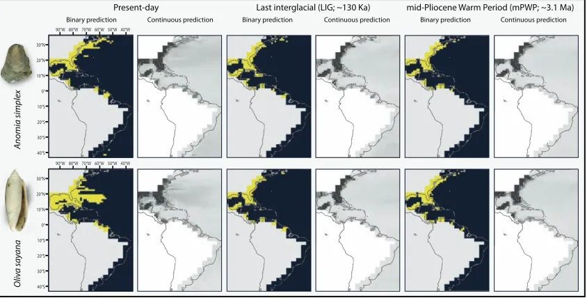
Figure 1 | Representative ecological niche models. Model results for the present, Last 728
Interglacial, and mid-Pliocene Warm Period for two species: Anomia simplex and Oliva
729
sayana. Binary and continuous predictions are presented, with binary predictions 730
thresholded using the mean suitability value from the continuous output. For the binary 731
predictions, yellow=suitable and dark blue=unsuitable, whereas for the continuous 732
predictions, darker greys indicate higher suitability. All analyses were conducted within 733
the geographic extent shown. Note that the modelled shorelines do not match the 734
continental shorelines because of the nature of our GCM data and the need to capture the 735
higher sea levels characteristic of the mid-Pliocene Warm Period.See electronic 736
supplementary material, figures S4-5, for remaining species analysed. 737
Anomia simplex
O
liv
a say
ana
Last interglacial (LIG; ~130 Ka)
Present-day mid-Pliocene Warm Period (mPWP; ~3.1 Ma)
Binary prediction Continuous prediction Binary prediction Continuous prediction Binary prediction Continuous prediction
30°N
20°N
10°N
0°
10°S
20°S
30°S
40°S
90°W 80°W 70°W 60°W 50°W 40°W
30°N
20°N
10°N
0°
10°S
20°S
30°S
40°S
90°W 80°W 70°W 60°W 50°W 40°W
738 739
740
741
742
743
744
745
746
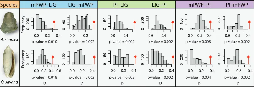
Figure 2 | Representative results from niche comparison analyses. Comparisons for 748
Anomia simplex and Oliva sayana using a PCA on the three most important 749
environmental variables: maximum and minimum surface temperature, and maximum 750
surface salinity. Comparisons are shown for the Last Interglacial (LIG, ~130 Ka), mid-751
Pliocene Warm Period (mPWP, ~3.1 Ma), and present-day (PI). The histograms show the 752
null distribution of similarity values (D) drawn from the study area, with the observed 753
similarity value in red. All comparisons indicate that niches are statistically more similar 754
than expected given the environmental backgrounds. For other comparisons, see table 1 755
and electronic supplementary material, table S3 and dataset S2. 756
A. simplex
O. sayana
LIG–mPWP
0.0 0.2 0.4
0
200
0.0 0.2
0
60
mPWP–LIG
0.0 0.4
0
150
0.0 0.4
0
200
PI–LIG LIG–PI
0.0 0.2 0.4
0
150
0.0 0.2 0.4
0
300
mPWP–PI PI–mPWP
Fr
equenc
y
Species
p-value = 0.002
p-value = 0.010 p-value = 0.002 p-value = 0.002 p-value = 0.008 p-value = 0.002
0.0 0.2 0.4 0.6
0
150
0.0 0.2 0.4
0
150
Fr
equenc
y
D D D D D D
0.0 0.2 0.4
0
150
0.0 0.2 0.4
0
100
0.0 0.2 0.4
0
200
0.0 0.2 0.4
0
200
p-value = 0.002 p-value = 0.002 p-value = 0.002 p-value = 0.004 p-value = 0.002
p-value = 0.018
757 758
759
760
761
762
763
764
765
766
767
768
769
770