This is a repository copy of On the influence of a translating inner core in models of outer core convection.
White Rose Research Online URL for this paper: http://eprints.whiterose.ac.uk/80886/
Version: Accepted Version
Article:
Davies, CJ, Silva, L and Mound, J (2013) On the influence of a translating inner core in models of outer core convection. Physics of the Earth and Planetary Interiors, 214. 104 - 114. ISSN 0031-9201
https://doi.org/10.1016/j.pepi.2012.10.001
[email protected] Reuse
Unless indicated otherwise, fulltext items are protected by copyright with all rights reserved. The copyright exception in section 29 of the Copyright, Designs and Patents Act 1988 allows the making of a single copy solely for the purpose of non-commercial research or private study within the limits of fair dealing. The publisher or other rights-holder may allow further reproduction and re-use of this version - refer to the White Rose Research Online record for this item. Where records identify the publisher as the copyright holder, users can verify any specific terms of use on the publisher’s website.
Takedown
If you consider content in White Rose Research Online to be in breach of UK law, please notify us by
On the influence of a translating inner core in models of outer core
convection
C. J. Daviesa,∗
, L. Silvaa, J. Mounda
a
School of Earth and Environment, University of Leeds, Leeds LS2 9JT, UK
Abstract
It has recently been proposed that the hemispheric seismic structure of the inner core can be explained by a self-sustained rigid-body translation of the inner core material, resulting in melting of the solid at the leading face and a compensating crystallisation at the trailing face. This process induces a hemispherical variation in the release of light elements and latent heat at the inner-core boundary, the two main sources of thermochemical buoyancy thought to drive convection in the outer core. However, the effect of a translating inner core on outer core convection is presently unknown. In this paper we model convection in the outer core using a nonmagnetic Boussinesq fluid in a rotating spherical shell driven by purely thermal buoyancy, incorporating the effect of a translating inner core by a time-independent spherical harmonic degree and order 1 (Y1
1) pattern of heat-flux imposed at the
inner boundary. The analysis considers Rayleigh numbers up to 10 times the critical value for onset of nonmagnetic convection, a parameter regime where the effects of the inhomogeneous boundary condition are expected to be most pronounced, and focuses on varying q∗
, the amplitude of the imposed boundary anomalies. The presence of inner boundary anomalies significantly affects the behaviour of the model system. Increasingq∗
leads to flow patterns dominated by azimuthal jets that span large regions of the shell where radial motion is significantly inhibited. Vigorous convection becomes increasingly confined to isolated regions asq∗
increases; these regions do not drift and always occur in the hemisphere subjected to a higher than average boundary heat-flux. Effects of the inner boundary anomalies are visible at the outer boundary in all models considered. At lowq∗
the expression of inner boundary effects at the core surface is a difference in the flow amplitude between the two hemispheres. As q∗
increases the spiralling azimuthal jets driven from the inner boundary are clearly visible at the outer boundary. Finally, our results suggest that, when the system is heated from below, a Y1
1 heat-flux pattern imposed on the inner boundary has a greater overall
influence on the spatio-temporal behaviour of the flow than the same pattern imposed at the outer boundary.
Keywords: Inner core translation, outer core convection, zonal flows, inhomogeneous heat-flux
∗Corresponding author
1. Introduction 1
Free thermal convection of the inner core, driven by either radiogenic heating (Jeanloz
2
and Wenk, 1988) or secular cooling (Buffett, 2009), has been proposed to explain the
ob-3
served cylindrical anisotropy in inner core P-wave velocity (Morelli et al., 1986; Woodhouse
4
et al., 1986). For this proposition to be viable the inner core must be (at least partially)
5
unstably stratified. Such a stratification may arise if the inner core temperature gradient
6
exceeds the adiabatic gradient at the relevant pressure-temperature conditions; previous
7
models suggest this may be true at present and was more likely in the past (Buffett, 2009;
8
Deguen and Cardin, 2009, 2011). Recent work suggests that the thermal conductivity of
9
the outer core is significantly higher than previously thought (Pozzo et al., 2012; de Koker
10
et al., 2012), which may affect the viability of thermal inner core convection, although these
11
calculations pertain to the liquid phase only. Another possibility is that the inner core is
12
compositionally unstable, which may arise if the amount of light element that remains in the
13
solid on freezing decreases with time (Deguen and Cardin, 2011; Alboussi`ere and Deguen,
14
2012). In reality the net inner core density gradient is determined by a combination of
15
thermal and chemical effects. Uncertainties in key parameters such the cooling rate at the
16
inner core boundary (ICB), the core-mantle boundary (CMB) heat-flux, and the partition
17
coefficients of the various light elements in the core prevent an unequivocal determination
18
of the inner core stratification and so inner core convection remains a realistic
possibil-19
ity. If the inner core does convect the preferred model likely depends on the bulk viscosity
20
(Deguen and Cardin, 2011). If the viscosity is sufficiently large the inner core could
un-21
dergo a translational mode of convection involving an eastward drift of inner core material
22
(Monnereau et al., 2010; Alboussi`ere et al., 2010). This mode has been used to explain an
23
observed asymmetry in seismic velocities between eastern and western hemispheres (Tanaka
24
and Hamaguchi, 1997; Niu and Wen, 2001; Waszek et al., 2011) and the existence of a
seis-25
mically slow layer in the bottom∼ 150 km of the outer core (Souriau and Poupinet, 1991;
26
Kennett et al., 1995; Zou et al., 2008).
27
Convection in the outer core is driven by a combination of thermal and chemical buoyancy
28
forces that in turn result from the Earth’s slow cooling (e.g. Buffett et al., 1996; Gubbins
29
et al., 2003, 2004). These buoyancy forces are likely to be strongest near the base of the
30
outer core (Davies and Gubbins, 2011) where inner core growth due to freezing of the liquid
31
iron alloy releases latent heat (Verhoogen, 1961), and a light component of the outer core
32
mixture, probably oxygen (Alf`e et al., 1999), remains in the liquid to provide a source of
33
compositional buoyancy (Braginsky, 1963). Models of outer core convection usually assume
34
that light element and latent heat release at the ICB are spherically symmetric and that
35
convection is driven uniformly from below (e.g. Braginsky and Roberts, 1995; Anufriev
36
et al., 2005); however, the translational mode of inner core convection requires freezing in
37
the western hemisphere and melting in the eastern hemisphere (Monnereau et al., 2010;
38
Alboussi`ere et al., 2010). The asymmetry arises because the eastward drift of inner core
39
material induces a west to east density gradient with heavy material on the freezing western
40
side; hydrostatic adjustment shifts the centre of mass of the inner core eastward so that the
41
eastern part of the inner core is above the melting temperature, leading to localised melting
(Alboussi`ere et al., 2010). Outer core convection is then driven non-uniformly from below:
43
in the western hemisphere, release of latent heat and light elements create outward buoyancy
44
fluxes that drive convection; in the eastern hemisphere, latent heat is absorbed and no light
45
elements are released, thereby creating a negative buoyancy flux.
46
In this paper we investigate the possible influence of a translating inner core on outer
47
core convection using a simple model of a rotating fluid-filled spherical shell. To incorporate
48
hemispherical variations induced by a translating inner core we note that the turnover time
49
of outer core convection,τc=d/U ∼102 yrs (Gubbins, 2007), is much shorter than both the 50
turnover time of the translational mode,τic =l/vt∼108 yrs, and the timescale for inner core 51
growth τg =l/vg ∼109 yrs (Labrosse et al., 2001). Here d is the outer core shell thickness, 52
U a characteristic outer core velocity, l the inner core radius, vt∼10
−10
m s−1
(Alboussi`ere
53
et al., 2010) a characteristic translational velocity and vg ∼ 10−11 m s−1 a characteristic 54
inner core growth rate. We therefore assume that, on the timescales associated with outer
55
core convection, both the ICB and the thermochemical anomalies resulting from translation
56
are stationary and can be modelled as a time-independent bottom boundary condition in the
57
outer core convection simulation. We further assume that this boundary condition takes the
58
form of a fixed flux. The outer core is well-mixed on timescales associated with inner core
59
convection, implying that the latter should be modelled with an isothermal and chemically
60
homogeneous ICB. Outer core convection must then respond to lateral variations in thermal
61
and chemical fluxes at the ICB induced by the translating inner core. The bottom boundary
62
condition is specified by the pattern and amplitude of thermochemical flux.
63
In this paper we approximate the pattern of hemispherical melting and freezing by a Y1 1 64
spherical harmonic. The amplitude of the anomaly is measured byq∗
, the ratio of the
peak-65
to-peak variation and the average flux through the boundary (see §2 for the mathematical
66
definition). Estimates of q∗
for the Earth are highly uncertain. The thermal contribution
67
depends on physical properties of the inner and outer cores, some of which are known to
68
within a factor of 3 at the relevant pressure-temperature conditions (Stacey, 2007), and
69
gross quantities such as the CMB heat-flux, which can only be estimated to within a factor
70
of 3–4 at present (Lay et al., 2009) and vary significantly over time (e.g. Nimmo et al.,
71
2004; Nimmo, 2007). The chemical contribution depends on the relative abundance of light
72
elements in both cores (i.e on the part of the ICB density jump not due to the phase change)
73
and on mixing properties of the core alloy, which are likely to be non-ideal (Helffrich, 2012)
74
and exhibit complex dependencies on partition coefficients (Alboussi`ere et al., 2010; Deguen
75
and Cardin, 2011).
76
A simple estimate of q∗
,q∗
e, can be obtained by neglecting chemical effects and assuming 77
that the only thermal buoyancy source at the ICB is latent heat (thus neglecting secular
78
cooling and the effect of the adiabat, both of which are likely to be smaller than the latent
79
heat (Davies and Gubbins, 2011)). The average ICB heat-flux per unit area, qL, is then 80
(Gubbins et al., 2003)
81
qL =ρiL
dri
dt =ρiLvg, (1)
where ri is the ICB radius, ρi the inner core density, and L the latent heat. An expression 82
(1). Assuming that the absolute value of the maximum and minimum heat-flux anomaly
84
are equal gives the estimate
85
q∗
e =
2vt
vg
. (2)
Using values from Alboussi`ere et al. (2010) gives present-day estimates in the range 1.q∗
e . 86
30 for a CMB heat-flux ranging from 8–11 TW. We vary q∗
in our simulations to exhibit
87
the dependence of the convection on this parameter.
88
This paper is organised as follows. In §2 we describe the numerical model used to
89
simulate convection in the outer core. In §3.1 we present models with a laterally-varying
90
Y1
1 inner boundary condition and a spherically symmetric outer boundary condition. We 91
discuss the changes in spatio-temporal behaviour that emerge as q∗
is varied and conduct a
92
detailed analysis of the mechanisms that drive large-scale flows in our models. In §3.2 we
93
briefly discuss models with a laterally-varyingY1
1 outer boundary condition and a spherically 94
symmetric inner boundary condition and compare to the results obtained in§3.1. Discussion
95
and conclusions are presented in§4.
96
2. Methods 97
We consider a model of convection in a rotating spherical shell that incorporates lateral
98
variations in the thermodynamic boundary conditions. A Boussinesq fluid of constant
ther-99
mal diffusivity,κ, constant coefficient of thermal expansion,α, and constant viscosity, ν, is
100
confined to a rotating spherical shell of thicknessd =ro−ri. Hereri andro are respectively 101
the inner and outer boundary radii in spherical polar coordinates, (r, θ, φ). The fluid rotates
102
about the axialz-axis with angular velocity Ω. To relate our results to previous studies and
103
to avoid double diffusive effects, which we regard as an unnecessary complication at this
104
stage, we consider a chemically homogeneous system heated from below, the analogue of
105
outer core convection driven by latent heat release at the inner boundary with no
composi-106
tional buoyancy. With no flow, the basic steady state temperature, T0, is maintained such 107
that∇T0 =−(β/r2)ˆr, whereβ measures the amplitude of the basic state radial temperature 108
gradient,r is the radial position vector and a hat denotes a unit vector. The total
tempera-109
ture field T =T0 +T
′
, where T′
is the deviation from the basic state temperature. Scaling
110
length by the shell thickness, d, time by the thermal diffusion time, d2/κ, and temperature 111
byβ/d, the nondimensional perturbation equations are
112
E P r
∂u
∂t + (u· ∇)u
+z×u = −∇P¯+RaT′r+E∇2u, (3)
∂T′
∂t + (u· ∇)T ′
= ∇2T′
+u·(βr−2)ˆr, (4)
∇ ·u = 0. (5)
The pressure gradient ∇P¯, is removed from the problem by taking the curl of (3). The
113
Ekman number E, Prandtl number P r, and modified Rayleigh number Ra are
114
E = ν
2Ωd2, P r=
ν
κ, Ra= αgβ
whereg is the gravitational acceleration at the outer boundary. Gravity varies linearly with
115
radius. The radius ratio, ri/ro, of the shell is set to 0.35. 116
The fluid velocity u is decomposed into toroidal and poloidal components,
117
u=∇ × Tr+∇ × ∇ × Pr. (7)
The toroidal, T, and poloidal, P, scalars along with the temperature T′
are expanded in
118
spherical harmonics Ym
l (θ, φ). The radial dependence of all variables is computed using 119
finite differences.
120
We use no-slip and impenetrable inner and outer boundaries, requiring
121
u(ri) =u(ro) = 0. (8)
We also fix the heat-flux on both boundaries. Lateral variations in heat-flux on the inner
122
boundary (IB) and outer boundary (OB) are modelled using the method described in
(Gib-123
bons et al., 2007). In all models the pattern of the boundary variation is a Y1
1 spherical 124
harmonic. The amplitude of the anomalies is measured by the parameter q∗
, defined as
125
the ratio of the peak-to-peak variation in boundary heat-flux and the average boundary
126
heat-flux
127
q∗ = qmax−qmin
q0
= 2qmax
q0
, (9)
whereqmax andqmin are the maximum and minimal values of the boundary anomaly. q0 is a 128
nondimensional measure of the average boundary heat-flux per unit area, q0 = (1/r2), and 129
is approximately a factor of 8 larger at the IB than at the OB. Hence, to impose the same
130
value ofqmax at the IB and OB requires that the value of q∗ is 8 times larger in the variable 131
OB heat-flux calculation compared to the variable IB heat-flux calculation.
132
The governing equations (3)–(5) are solved using a pseudo-spectral method. Detailed
133
descriptions of the code are given in Willis et al. (2007) and Davies et al. (2011).
134
3. Results 135
Table 1 lists all simulations conducted for this work. In order to facilitate comparisons
136
and to elucidate the effect of the laterally-varying IB condition, we fix the values ofEandP r
137
and varyRaandq∗
. For simplicity we use the valueP r= 1 throughout. The Ekman number
138
is the major computational challenge. The lowest value ofE used in a numerical simulation
139
is∼5×10⁻⁷(Kageyama et al., 2008); very few models have been conducted in this parameter 140
regime, which is still many orders of magnitude higher than the valueE ∼10−15
appropriate
141
to Earth’s outer core. We fix E = 10−5, which is low enough for rotation to dominate in 142
our calculations but high enough to conduct a suite of simulations run for long enough
143
to obtain time-averages that span many time units. At this value of E a linear stability
144
analysis (see Gibbons et al. (2007) and Davies et al. (2009) for details) with our chosen
145
boundary conditions and value ofP r shows that the most unstable azimuthal wavenumber,
146
mc = 9, and the corresponding value of the critical Rayleigh number, Rac = 25.5, for the 147
onset of non-magnetic convection with homogeneous boundaries (q∗
= 0). We focus on the
parameter range 3Rac ≤Ra≤10Rac, where we expect the influence of the inhomogeneous 149
boundary condition to be most pronounced. If boundary effects are not important in this
150
regime we would anticipate that they be less significant in the core whereRais likely to be
151
many times supercritical (Gubbins, 2001; Davies and Gubbins, 2011).
152
All simulations were started from the same initial condition with u = 0 and arbitrary
153
three dimensional seed perturbations superimposed on the basic state temperature profile.
154
The spatial resolution required to achieve a given level of spectral convergence increases with
155
Ra. At the lowest values of Ra we found thatNmax = 90 radial points and maximum har-156
monic degreeLmax = 84 produced a drop of four orders of magnitude between wavenumbers 157
with highest and lowest energy. At the highest values of Ra, Nmax = 120 and Lmax = 128 158
were required to obtain the same convergence.
159
For the subsequent discussion we define the dimensionless kinetic energy K =KT +KP,
160
where the toroidal and poloidal components are given respectively by
161
KT =
1 2
|∇ × Tr|2 ,
KP =
1 2
|∇ × ∇ × Pr|2 ,
and angled brackets indicate a time average over the length of the run quoted in Table 1.
162
The zonal part of the toroidal energy,Kz
T, is obtained by retaining only them = 0 harmonic
163
coefficient.
164
Our choice of nondimensionalisation means that the P´eclet number, P e = U d/κ =
165
p
2K/Vs, where Vs is the volume of the spherical shell, measures the amplitude of the 166
velocity U. With all other parameters fixed, increasing Ra leads to an increase inP e while
167
the ratios KT/K and KTz/K remain relatively constant in the parameter range considered
168
(Table 1). Increasingq∗
with all other parameters fixed shows a general increase inP e (see
169
also Figure 1), a slight increase in KT/K and little variation in KTz/K, which is a small
170
fraction of the total energy in all models.
171
In the next two sections we analyse the models in Table 1 in detail. In the subsequent
172
discussion φ = 0◦
corresponds to the rightmost edge of the equatorial projections and is
173
the longitude of minimum heat-flux; the maximum heat-flux is imposed at φ = 180◦
. The
174
western hemisphere, which is subject to a higher than average heat-flux, is defined as the
175
region 90◦
< φ ≤ 270◦
and the eastern hemisphere, which is subjected to a lower than
176
average heat-flux, is defined as the region −90◦
< φ≤90◦
.
177
3.1. Y1
1 inner boundary condition 178
Figure 2 shows four models with Ra = 90 that differ only by the value of q∗
. The
179
snapshots are taken at time t = 11 of Figure 1a. With homogeneous boundaries (q∗
= 0)
180
the familiar pattern of spiralling columnar rolls aligned with the rotation axis, a feature of
181
moderate P r and low Ra convection, is obtained (Zhang, 1992). The prograde drift speed
182
of the columns varies with radius and hence the convection is characterised by different
183
wavenumbers at different distances from the rotation axis (e.g. Sun et al., 1993; Tilgner
and Busse, 1997). The pattern of temperature anomalies in the equatorial plane is
well-185
correlated with radial velocity. Them-spectrum of kinetic energy (Figure 1) is characterised
186
by a peak atm = 0, and broad peaks around the most unstable mode and its overtones.
187
Imposing a Y1
1 heat-flux variation at the inner boundary significantly alters the large-188
scale flow pattern as q∗
is increased above zero. For Ra= 90 we identify three broad flow
189
regimes. For q∗
≤ 0.6 the homogeneous flow pattern is modulated by the presence of the
190
Y1
1 boundary anomaly. Figure 2 shows that, for q
∗
= 0.6, the velocity field in the western
191
hemisphere has a higher amplitude and a larger characteristic azimuthal wavenumber than
192
in the eastern hemisphere. The columnar rolls drift in the prograde sense in this model,
193
but accelerate when passing through the eastern (low heat-flux) hemisphere and decelerate
194
when passing through the western hemisphere. Similar behaviour was found by Zhang
195
and Gubbins (1993) in a convection model with lateral variations at the OB. Temperature
196
anomalies near the IB are predominantly negative in the region 0◦
< φ≤180◦
and positive
197
in the region 180◦
< φ≤ 360◦
; a similar phase shift of temperature anomalies with respect
198
to the boundary anomalies has been observed in models of convection with lateral OB
199
variations (Olson, 2003).
200
For 0.6< q∗
≤1.4 them= 1 mode becomes dominant in the m-spectrum of the kinetic
201
energy (Figure 1) and convection columns are absent in parts of the eastern hemisphere.
202
Very weak radial motions are observed between −90◦
< φ ≤ 0◦
as shown in Figure 2 for
203
q∗
= 1.4. This region is characterised by strong prograde and retrograde azimuthal jets that
204
are established near the IB at φ ≈ 180◦
and spiral outwards, terminating when they reach
205
the OB. Strong vertical and radial gradients in azimuthal velocity are evident in the region
206
spanned by the jets. The pattern of temperature anomalies is dominated by an m = 1
207
component and strong gradients in the region where the jets are formed.
208
Finally, for q∗
>1.4 the flow patterns are almost stationary as suggested by the kinetic
209
energy time-series in Figure 1a. Figure 2 for q∗
= 4.2 shows that the azimuthal jets become
210
stronger and have greater lateral extent than at lower values ofq∗
. The amplitude of vertical
211
and radial gradients in azimuthal velocity in the region spanned by the jets also increase
212
with q∗
. Strong upwelling and downwelling regions are visible in the plot of ur near the 213
locations where the azimuthal jets are initiated and terminated due to interaction with the
214
OB, but away from these regions the radial velocity is very weak. Temperature gradients
215
are strong in the region where the azimuthal jets are formed and departures from the basic
216
state are significant across broad regions of the shell.
217
The large-scale flow patterns described above forq∗
≥1.4 are reminiscent of those found
218
by Grote and Busse (2001) and Busse et al. (2003) in simulations of rotating convection
219
with homogeneous boundaries. In their models, convection columns are sheared by a strong
220
azimuthal zonal (m= 0) flow driven by Reynolds stresses; the zonal flow dominates in large
221
regions of the shell where radial motion is severely inhibited. Although a large-scale shear is
222
apparent in our models for q∗
≥1.4 there are three factors suggesting that it is driven by a
223
different mechanism to that described by Grote and Busse (2001). Firstly, our values ofRa
224
are much smaller than those used by Grote and Busse (2001); indeed, with a homogeneous
225
IB condition and Ra = 90, Figure 2 shows that convection columns are not confined to a
226
particular longitudinal band. Secondly, the region where convection columns are observed in
the Grote and Busse (2001) simulations is not fixed in space, in contrast to our models where
228
this region remains in the western hemisphere. Finally, our models contain only ∼1/10th
229
of the total energy in zonal components (Table 1), suggesting that the shear generated by
230
large-scale nonzonal flows could greatly exceed shear generated by the zonal flow. We now
231
explore these three points in detail by investigating the mechanisms that drive the azimuthal
232
flows observed forq∗
≥1.4 (Figure 2). We first consider the azimuthal zonal flow, which we
233
denoteuz
φ, and then focus on the nonzonal azimuthal flow, which is denotedunzφ hereafter. 234
There are two main driving mechanisms for uz
φ (e.g. Cardin and Olson, 1994; Aubert 235
et al., 2003). The first is due to Reynolds stresses arising from the convection columns,
236
which drive a zonal flow with cylindrical symmetry that tends to be strongly retrograde
237
near the IB (Busse, 1970; Cardin and Olson, 1994) and slightly retrograde (Cardin and
238
Olson, 1994) or prograde (Glatzmaier and Olson, 1993) near the OB. The second driving
239
force foruz
φ arises because more heat is lost in equatorial regions than polar regions, which 240
sets up axisymmetric latitudinal temperature gradients that drive zonal flows with shear in
241
the verticalz direction. To distinguish between these two mechanisms we follow Glatzmaier
242
and Olson (1993) and define the geostrophic wind as the portion of the zonal flow that
243
is uniform in the axial direction and the remainder, which contains vertical shear, as the
244
ageostrophic wind. We computeuz
φ by retaining only them = 0 component of the velocity 245
field, and the geostrophic wind, [u]z
φ by averaging this flow over z. The averaging operation 246
denoted by square brackets is defined by
247
[] = 1 2L
Z −L
L
dz, L=pr2
o−s2, (10)
where s = rsin(θ) is cylindrical radius. Figure 3 shows uz
φ and [u]zφ for q
∗
= 1.4 and 4.2.
248
The zonal flow is westward (retrograde) near the tangent cylinder (the imaginary cylinder
249
parallel to the rotation axis that touches the inner core equator) for all values ofq∗
including
250
q∗
= 0. Near the OB,uz
φis slightly prograde at mid-latitudes for low values ofq
∗
; forq∗
≥2.8
251
the progradeuz
φ at mid-latitudes is approximately half the value of the retrograde flow near 252
the IB. These features are also reflected in the profiles of [u]z
φ in Figure 3. Increasing q
∗
253
produces a mild increase inuz
φ, presumably due to nonlinear interaction with the large-scale 254
boundary forcing, and also causes an increase in [u]z
φ; the ratio [u]zφ/uzφ does not show a 255
strong dependence on q∗
for the particular Ra we have considered. We conclude that, for
256
the models considered, the geostrophic and ageostrophic contributions to the zonal flow are
257
comparable.
258
Our models contain a large-scale nonzonal azimuthal flow, unz
φ , that dramatically in-259
creases in amplitude as q∗
increases (compare the meridional sections in Figures 2 and 3).
260
The variation of uφ with z seen in both Figures suggests a significant thermal wind exists 261
in our models, as has been found in other simulations with inhomogeneous boundary
condi-262
tions (e.g. Zhang, 1992; Sreenivasan, 2009). Taking the curl of equation (3) with the viscous
263
force and acceleration term omitted gives
264
∂u
∂z +Ra∇ ×(Tr)− E
omitting the contribution from the divergence of the Reynolds stress (the last term) gives
265
the thermal wind balance. Figure 4 shows the terms in (11) and their sum for q∗
= 4.2.
266
For this model the first two terms in (11) are over an order of magnitude larger than the
267
last term. The remainder after summing terms on the left-hand side of (11) is close to zero
268
outside the tangent cylinder as shown in the rightmost column of Figure 4. These results
269
imply that a thermal wind balance holds for the model withq∗
= 4.2. Further calculations
270
(not shown) indicate that this balance holds well for all models conducted at Ra = 90.
271
Sumita and Olson (2002) noted that regions where ∂uφ/∂z > 0 and where |uφ| decreases 272
with z imply uφ < 0 if the thermal wind balance applies. Similarly, ∂uφ/∂z > 0 and |uφ| 273
increasing with z implies uφ > 0; ∂uφ/∂z < 0 and |uφ| decreasing with z implies uφ > 0; 274
∂uφ/∂z < 0 and |uφ| increasing with z implies uφ < 0. The meridional sections shown in 275
Figure 5 for q∗
= 4.2 indicate that the above relations are reasonably well-satisfied and
276
further calculations for models that contain large-scale azimuthal jets (see Figure 2) give
277
similar results. These results suggest that, in the models described above, the dominant
278
driving force for the nonzonal azimuthal flow,unz
φ , is a thermal wind. Furthermore, Figure 4 279
indicates that a thermal wind is the dominant driving force for the ageostrophic contribution
280
to the azimuthal zonal flow,uz φ. 281
Figures 3 and 5 show that changes in sign ofuz
φ andunzφ occur at almost the same (cylin-282
drical) radii in regions where radial flow is weak and azimuthal flow dominates, suggesting
283
that shear due to the zonal flow is reinforced by shear due to the nonzonal azimuthal flow
284
driven by the inhomogeneous boundary. This explains why convection columns are not
con-285
fined to a particular longitudinal band in models with no boundary forcing: shear in the
286
zonal flow alone is not strong enough to break down the convection columns. The region
287
where the columnar rolls can persist is determined by the amplitude of the shear produced
288
byuz
φ andunzφ . Forq
∗
≥2.8,ur andunzφ are both strongest above the maximum IB heat-flux 289
at φ = 180◦
, but the shear due to the strong unz
φ is sufficient to break down convection 290
columns directly east of the maximum heat-flux until unz
φ weakens sufficiently for columns 291
to reemerge around φ = 0◦
. At lower values of q∗
the unz
φ driven by the thermal wind is 292
not strong enough to shear convection columns in the western hemisphere where the high
293
heat-flux drives strong radial motions; however, in the eastern hemisphere, the combined
294
action of zonal and nonzonal azimuthal flows dominates over the relatively weak radial
mo-295
tions. This explains why the region where convection columns persist is always located in the
296
hemisphere where the IB heat-flux is higher than the average. Finally, our analysis suggests
297
that the large-scale azimuthal flows in the models described above are driven predominantly
298
by a thermal wind; Reynold’s stresses play a secondary role.
299
For Ra= 150 and Ra = 225 we did not obtain quasi-stationary solutions for any value
300
ofq∗
considered. Higher values ofRalead to more energy in small-scales compared to those
301
with Ra = 90, but the large-scale features are very similar to those described above for
302
Ra= 90. Figure 6 shows time-averaged flow patterns withq∗
= 1.4 and Ra= 90,150,225.
303
Instantaneous and time-averaged flows forRa= 90 show the same basic features, as could be
304
anticipated by comparing the time-averaged and instantaneous velocity spectra in Figure 1.
305
Interestingly, the time-averaged flow forq∗
= 1.4 indicates that upwellings and downwellings
306
in the western hemisphere, with a characteristic lengthscale much smaller than that of the
imposed boundary anomaly, occur in preferred locations. The superposition of scales in
308
flows forced by inhomogeneous outer boundary conditions was noted by Davies et al. (2009).
309
Equatorial sections forRa= 150 and 225 reveal large-scale nonzonal azimuthal flows similar
310
to those studied in detail for Ra= 90 and q∗
= 4.2; indeed, applying the same analysis to
311
these cases suggests that the mechanisms inferred to drive the zonal azimuthal flowuz φ, and 312
the nonzonal azimuthal flow unz
φ , are the same as those discussed for models withRa= 90. 313
IncreasingRafor fixedq∗
does not change the amplitude ofunz
φ significantly, but strengthens 314
uz
φ (Table 1) due to increased Reynolds stresses and axisymmetric latitudinal temperature 315
gradients. The combined shear due to uz
φ and unzφ (which are well-correlated as above) 316
produces similar large-scale effects at Ra= 150,225 as for Ra= 90. These results suggest
317
that the behaviour described for solutions with Ra = 90 is broadly characteristic of the
318
behaviour across the range ofRa considered.
319
3.2. Y1
1 outer boundary condition 320
In this section we briefly discuss the effect of imposing aY1
1 boundary anomaly at the OB 321
with a homogeneous IB. The model parameters are the same as used in§3.1, but we consider
322
only Ra = 90 . Simulations were conducted with q∗
= 11.2 and q∗
= 34.2 (see Table 1),
323
corresponding to OB anomalies that are equal in magnitude to the IB anomalies imposed in
324
the models with q∗
= 1.4 and 4.2 respectively. No quasi-steady solutions were obtained for
325
models withY1
1 OB anomalies at Ra= 90, unlike models with Y11 IB anomalies where such 326
solutions were obtained for Ra= 90 andq∗
≥2.8. Simulations at higher values of Ra were
327
not conducted, but quasi-steady solutions are not anticipated based on the results of §3.1.
328
Figure 7 shows a snapshot of the flow pattern for Ra = 90 and q∗
= 34.2. Temporal
329
variations are most apparent outside the tangent cylinder near the IB, where a sequence of
330
columnar rolls reminiscent of the pattern of homogeneous (q∗
= 0) convection (see Figure 2)
331
drift predominantly in the prograde sense. A cluster of rolls are located beneath the OB
332
under the region of high heat-flux and remain in this location for the length of our simulation
333
(6 time units). A previous study (Davies et al., 2009) with an imposed Y2
2 OB condition 334
found two such clusters. These results suggest that the number of clusters is determined
335
by the azimuthal wavenumber of the imposed boundary anomaly. Large-scale nonzonal
336
azimuthal flows are generated near the OB but do not penetrate all the way to the IB.
337
Figure 8 shows theφ-component of the thermal wind balance (equation (11)) forRa= 90
338
and q∗
= 34.2. Both terms are large and tend to balance near the OB; however, the
339
amplitude of the thermal wind decreases significantly with depth. Conducting the analysis
340
of§3.1 suggests that the large-scale nonzonal azimuthal flows near the OB are driven by the
341
thermal wind resulting from the OB heat-flux anomalies; these flows are much stronger than
342
those obtained with aY1
1 IB condition (see Table 1), which we attribute to the larger surface 343
area of the OB giving rise to a stronger thermal wind. Azimuthal flows are much weaker and
344
contain more small-scale structure at depth where the thermal wind is weak. This, together
345
with the fact that the homogeneous system is driven from below, suggests that the effects
346
of OB anomalies do not penetrate far enough into the shell to stop fluid near the IB from
347
drifting, as it would do in the absence of boundary anomalies. For this particular model
348
it appears that the Y1
characteristics of the flow than aY1
1 IB condition. We attribute this to the fact that, in our 350
simulations, the IB condition is imposed in the same location as the buoyancy source for
351
free convection.
352
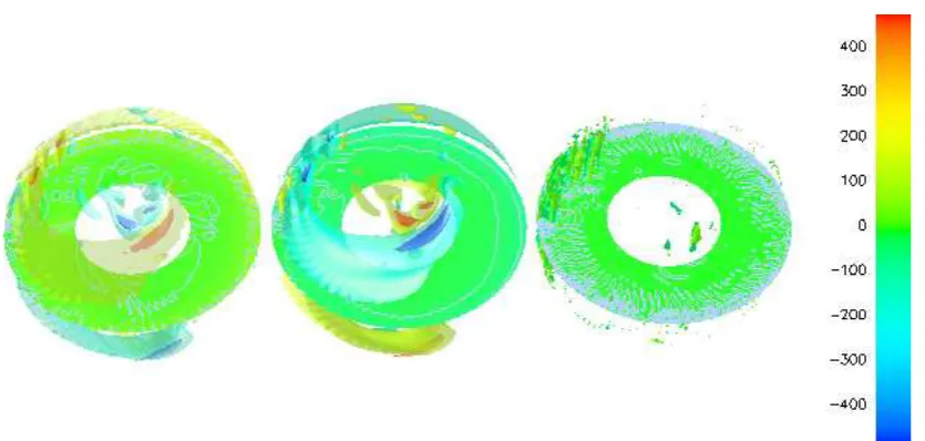
4. Discussion and conclusions 353
We have performed numerical simulations to investigate the effects of a translating inner
354
core on outer core convection. The novel feature of our model is that convection in the
355
outer core is driven non-uniformly from below. Many previous studies have investigated the
356
effects of laterally-varying outer boundary conditions on rotating convection (e.g. Zhang,
357
1992; Zhang and Gubbins, 1993; Davies et al., 2009) and magnetic field generation (e.g.
358
Olson and Christensen, 2002; Willis et al., 2007; Sreenivasan, 2009) in spherical shells. By
359
contrast, laterally-varying inner boundary conditions have received very little attention, save
360
for an investigation into possible long-term asymmetry in the geomagnetic field by Olson
361
and Deguen (2012). Studies with laterally-varying outer boundary conditions generally use
362
a pattern of boundary anomalies inferred from seismic tomography, a complex combination
363
of spherical harmonics, or the largest harmonic in this pattern, which isY2
2. Conversely, the 364
large-scale pattern imposed by inner core translation is a spherical harmonicY1
1. Motivated 365
by these issues, we used an idealised nonmagnetic model of thermally-driven convection in
366
a rotating spherical shell designed to highlight the effects of the imposedY1
1 inner boundary 367
heat-flux. Nonmagnetic models reduce computational costs, allowing a suite of simulations
368
to be conducted, and afford theoretical simplifications compared to geodynamo simulations.
369
Our results for the simpler hydrodynamic problem will hopefully guide future research into
370
geodynamo models with laterally-varying inner boundary conditions.
371
The suite of simulations conducted for this work use an Ekman number that is low enough
372
for the dynamics to be rotation-dominated and focus on low Rayleigh numbers, where the
373
influence of the boundary condition is expected to be prominent. Higher Rayleigh numbers
374
could lead to a weakening of boundary effects at the values of q∗
(which measures the
375
amplitude of boundary anomalies) used in this work, but higher values of q∗
may lead to
376
significant boundary effects even when the Rayleigh number is highly supercritical. Such a
377
regime cannot be ruled out given the significant uncertainties in the value ofq∗
appropriate
378
for the Earth.
379
In our models, increasingq∗
with all other parameters fixed leads to significant changes in
380
the large-scale flow pattern compared to the solution with a homogeneous inner boundary
381
(q∗
= 0). The most striking feature is the development of spiralling azimuthal jets that
382
span large portions of the shell. Radial motion tends to be weak where the azimuthal jets
383
are strong. Vigorous convection becomes increasingly confined to localised regions as q∗
384
increases; these regions do not drift and are always located in the hemisphere where the
385
boundary heat-flux is higher than the average.
386
We explored the processes responsible for generating the localised regions of convection
387
that emerge at large q∗
, focusing on shear generated by the large-scale zonal and nonzonal
388
azimuthal flows. Zonal flows generally account for only a small fraction of the total kinetic
389
energy in our models, partly due to our use of no-slip boundary conditions (Christensen,
2002) and partly due to choice of relatively lowRa. The energy in the zonal flow remains a
391
small fraction of the kinetic energy for all values ofq∗
considered. Large-scale nonzonal
az-392
imuthal jets significantly increase in amplitude withq∗
and tend to dominate the zonal flows
393
when the boundary forcing is strong. Our analysis suggests that the large-scale nonzonal
394
azimuthal jets are driven by a thermal wind resulting from the boundary anomalies and that
395
the shear generated by these jets leads to the destruction of columnar convection rolls (that
396
would otherwise exist in the absence of boundary anomalies) in regions where the shearing
397
flow is much greater than the amplitude of the radial flow. Thermal winds were found to be
398
more important for driving large-scale flows than Reynold’s stresses at high values ofq∗
.
399
Applying a Y1
1 heat-flux pattern at the outer boundary, with a spherically symmetric 400
inner boundary, appears to exert a weaker influence on fluid far from the inhomogeneous
401
boundary compared to a model with the same parameter values and a Y1
1 inner boundary 402
condition. We suggest that this occurs in the model because outer boundary effects are
403
weakest where the buoyancy force driving homogeneous convection is strongest. Models
404
with inhomogeneous inner and outer boundaries designed to simulate outer core-mantle and
405
outer core-inner core interactions are needed to further explore this potentially significant
406
result.
407
The effects of the inner boundary condition are visible in instantaneous and time-averaged
408
surface flows even for low values of q∗
. Figure 9 shows that the surface expression of the
409
lateral inner boundary anomalies is an amplitude difference between the flow in the eastern
410
and western hemispheres. The amplitude difference increases withq∗
. At the highest values
411
of q∗
there is a clear signature of the large-scale azimuthal flows that are generated near
412
the inner boundary and spiral outward. Close correspondence between magnetic and
non-413
magnetic flows found in models with laterally-varying outer boundary conditions (e.g. Willis
414
et al., 2007) raise the possibility that flows of this type may arise in geodynamo models.
415
This may be the case if the Lorentz force does not significantly alter the largest scales of
416
the flow.
417
Our principle conclusion is that the presence of thermal inner boundary anomalies can
418
significantly affect the dynamics of convection in a rotating spherical shell. This result
419
appears consistent with the models of Olson and Deguen (2012), which include the effect
420
of a magnetic field but operate at lower rotation rates than those considered here. Future
421
work is needed to assess the role of laterally-varying thermal inner boundary conditions at
422
rapid rotation rates with the inclusion of the magnetic field.
423
Acknowledgements 424
C.D. is supported by a Natural Environment Research Council personal fellowship,
425
NE/H01571X/1. L.S. and J.M. are funded by the Natural Environment Research
Coun-426
cil through grant NE/G002223/1. The authors thank Dr. P. Livermore for stimulating
427
discussions.
References 429
Alboussi`ere, T., Deguen, R., 2012. Asymmetric dynamics of the inner core and impact on the outer core. J.
430
Geodyn. In Press.
431
Alboussi`ere, T., Deguen, R., Melzani, M., 2010. Melting-induced stratification above the Earth’s inner core
432
due to convective translation. Nature 466, 744–747.
433
Alf`e, D., Price, G. D., Gillan, M. J., 1999. Oxygen in the Earth’s core: a first-principles study. Phys. Earth
434
Planet. Int. 110, 191–210.
435
Anufriev, A., Jones, C., Soward, A., 2005. The Boussinesq and anelastic liquid approximations for convection
436
in Earth’s core. Phys. Earth Planet. Int. 152, 163–190.
437
Aubert, J., Gillet, N., Cardin, P., 2003. Quasigeostrophic models of convection in rotating spherical shells.
438
Geochem. Geophys. Geosys. 4.
439
Braginsky, S., 1963. Structure of the F layer and reasons for convection in the Earth’s core. Sov. Phys. Dokl.
440
149, 8–10.
441
Braginsky, S., Roberts, P., 1995. Equations governing convection in Earth’s core and the geodynamo.
Geo-442
phys. Astrophys. Fluid Dyn. 79, 1–97.
443
Buffett, B., 2009. Onset and orientation of convection in the inner core. Geophys. J. Int. 179, 711–719.
444
Buffett, B., Huppert, H., Lister, J., Woods, A., 1996. On the thermal evolution of the Earth’s core. J.
445
Geophys. Res. 101, 7989–8006.
446
Busse, F., 1970. Differential rotation in stellar convection zones. Astrophys. J. 159, 629–639.
447
Busse, F., Grote, E., Simitev, R., 2003. Convection in rotating spherical shells and its dynamo action. In:
448
Earth’s core and lower mantle. Contributions from the SEDI 2000, The 7th Symposium, pp. 130–152.
449
Cardin, P., Olson, P., 1994. Chaotic thermal convection in a rapidly rotating spherical shell: consequences
450
for flow in the outer core. Phys. Earth Planet. Int. 82, 235–259.
451
Christensen, U., 2002. Zonal flow driven by strongly supercritical convection in rotating spherical shells. J.
452
Fluid Mech. 470, 115–133.
453
Davies, C., Gubbins, D., 2011. A buoyancy profile for the Earth’s core. Geophys. J. Int. 187, 549–563.
454
Davies, C., Gubbins, D., Jimack, P., 2009. Convection in a rapidly rotating spherical shell with an imposed
455
laterally varying thermal boundary condition. J. Fluid Mech. 641, 335–358.
456
Davies, C., Gubbins, D., Jimack, P., 2011. Scalability of pseudospectral methods for geodynamo simulations.
457
Concurrency Computat.: Pract. Exper. 23, 38–56.
458
de Koker, N., Steinle-Neumann, G., Vojtech, V., 2012. Electrical resistivity and thermal conductivity of
459
liquid Fe alloys at high P and T and heat flux in Earth’s core. Proc. Natl. Acad. Sci. 109, 4070–4073.
460
Deguen, R., Cardin, P., 2009. Tectonic history of the Earth’s inner core preserved in its seismic structure.
461
Nat. Geosci. 2, 419–422.
462
Deguen, R., Cardin, P., 2011. Thermochemical convection in Earth’s inner core. Geophys. J. Int. 187, 1101–
463
1118.
464
Gibbons, S., Gubbins, D., Zhang, K., 2007. Convection in a rotating spherical shell with inhomogeneous
465
heat flux at the outer boundary. Geophys. Astrophys. Fluid Dyn. 101, 347–370.
466
Glatzmaier, G., Olson, P., 1993. Highly supercritical thermal convection in a rotating spherical shell:
cen-467
trifugal vs. radial gravity. Geophys. Astrophys. Fluid Dyn. 70, 113–136.
468
Grote, E., Busse, F., 2001. Dynamics of convection and dynamos in rotating spherical fluid shells. Fluid
469
Dyn. Res. 28, 349–368.
470
Gubbins, D., 2001. The Rayleigh number for convection in the Earth’s core. Phys. Earth Planet. Int. 128,
471
3–12.
472
Gubbins, D., 2007. Dimensional analysis and timescales for the geodynamo. In: Gubbins, D.,
Herrero-473
Bervera, E. (Eds.), Encyclopedia of Geomagnetism and Paleomagnetism. Springer, pp. 287–300.
474
Gubbins, D., Alfe, D., Masters, G., Price, G., Gillan, M., 2003. Can the Earth’s dynamo run on heat alone?
475
Geophys. J. Int. 155, 609–622.
476
Gubbins, D., Alfe, D., Masters, G., Price, G., Gillan, M., 2004. Gross thermodynamics of two-component
477
core convection. Geophys. J. Int. 157, 1407–1414.
Helffrich, G., 2012. How light element addition can lower core liquid wave speeds. Geophys. J. Int., 1065–
479
1070.
480
Jeanloz, R., Wenk, H., 1988. Convection and anisotropy of the inner core. Geophys. Res. Lett. 15, 72–75.
481
Kageyama, A., Miyagoshi, T., Sato, T., 2008. Formation of current coils in geodynamo simulations. Nature
482
454, 1106–1109.
483
Kennett, B., Engdahl, E., Buland, R., 1995. Constraints on seismic velocities in the Earth from traveltimes.
484
Geophys. J. Int. 122, 108–124.
485
Labrosse, S., Poirier, J.-P., Le Moeul, J.-L., 2001. The age of the inner core. Earth Planet. Sci. Lett. 190,
486
111–123.
487
Lay, T., Hernlund, J., Buffett, B., 2009. Core-mantle boundary heat flow. Nat. Geosci. 1, 25–32.
488
Monnereau, M., Calvet, M., Margerin, L., Souriau, A., 2010. Lopsided growth of Earth’s inner core. Science
489
328, 1014–1017.
490
Morelli, A., Dziewonski, A., Woodhouse, J., 1986. Anisotropy of the inner core inferred from PKIKP travel
491
times. Geophys. Res. Lett. 13 (13), 1545–1548.
492
Nimmo, F., 2007. Thermal and compositional evolution of the core. In: Schubert, G. (Ed.), Treatise on
493
Geophysics, Vol. 8. Elsevier, Amsterdam, pp. 217–241.
494
Nimmo, F., Price, G., Brodholt, J., Gubbins, D., 2004. The influence of potassium on core and geodynamo
495
evolution. Geophys. J. Int. 156, 363–376.
496
Niu, F., Wen, L., 2001. Hemispherical variations in seismic velocity at the top of the Earth’s inner core.
497
Nature 410, 1081–1084.
498
Olson, P., 2003. Thermal interaction of the core and mantle. In: Earth’s core and lower mantle. Contributions
499
from the SEDI 2000, The 7th Symposium, pp. 1–38.
500
Olson, P., Christensen, U., 2002. The time-averaged magnetic field in numerical dynamos with non-uniform
501
boundary heat flow. Geophys. J. Int. 151, 809–823.
502
Olson, P., Deguen, R., 2012. Eccentricity of the geomagnetic dipole caused by lopsided inner core growth.
503
Nat. Geosci. 5, 565–569.
504
Pozzo, M., Davies, C., Gubbins, D., Alf`e, D., 2012. Thermal and electrical conductivity of iron at Earth’s
505
core conditions. Nature 485, 355–358.
506
Souriau, A., Poupinet, G., 1991. The velocity profile at the base of the liquid core from PKP(BC+Cdiff)
507
data: an argument in favor of radial inhomogeneity. Geophys. Res. Lett. 18, 2023–2026.
508
Sreenivasan, B., 2009. On dynamo action produced by boundary thermal coupling. Phys. Earth Planet. Int.
509
177, 130–138.
510
Stacey, F., 2007. Core properties, physical. In: Gubbins, D., Herrero-Bervera, E. (Eds.), Encyclopedia of
511
Geomagnetism and Paleomagnetism. Springer, pp. 91–94.
512
Sumita, I., Olson, P., 2002. Rotating thermal convection experiments in a hemispherical shell with
hetero-513
geneous boundary heat flux: Implications for the Earth’s core. J. Geophys. Res. 107.
514
Sun, Z.-P., Schubert, G., Glatzmaier, G., 1993. Transitions to chaotic thermal convection in a rapidly
515
rotating spherical fluid shell. Geophys. Astrophys. Fluid Dyn. 69, 95–131.
516
Tanaka, S., Hamaguchi, H., 1997. Degree one heterogeneity and hemispherical variation of anisotropy in the
517
inner core from PKP(BC)-PKP(DF) times. J. Geophys. Res. 102, 2925–2938.
518
Tilgner, A., Busse, F., 1997. Finite-amplitude convection in rotating spherical fluid shells. J. Fluid Mech.
519
332, 359–376.
520
Verhoogen, J., 1961. Heat balance of the Earth’s core. Geophys. J. R. Astr. Soc. 4, 276–281.
521
Waszek, L., Irving, J., Deuss, A., 2011. Reconciling the hemispherical structure of Earth’s inner core with
522
its super-rotation. Nat. Geosci. 4, 264–267.
523
Willis, A., Sreenivasan, B., Gubbins, D., 2007. Thermal core-mantle interaction: exploring regimes for
524
‘locked’ dynamo action. Phys. Earth Planet. Int. 165, 83–92.
525
Woodhouse, J., Giardini, D., Li, X.-D., 1986. Evidence for inner core anisotropy from free oscillations.
526
Geophys. Res. Lett. 13, 1549–1552.
527
Zhang, K., 1992. Convection in a rapidly rotating spherical shell at infinite Prandtl number: transition to
528
vacillating flows. Phys. Earth Planet. Int. 72, 236–248.
Zhang, K., Gubbins, D., 1993. Convection in a rotating spherical fluid shell with an inhomogeneous
tem-530
perature boundary condition at infinite Prandtl number. J. Fluid Mech. 250, 209–232.
531
Zou, Z., Koper, K., Cormier, V., 2008. The structure of the base of the outer core inferred from seismic
532
waves diffracted around the inner core. J. Geophys. Res. 113, B05314.
Ra q∗
P e KT (KT/K) KTz (KTz/K)
90 0 38.6 8851 (0.82) 1529 (0.14)
90 0.3 37.2 8162 (0.81) 1258 (0.12)
90 0.6 39.1 9093 (0.82) 1342 (0.12)
90 1.4 45.1 12534 (0.84) 1571 (0.10)
90 2.8 58.2 21689 (0.88) 4014 (0.16)
90 4.2 62.2 24784 (0.88) 4372 (0.16)
90* 11.4 62.8 23972 (0.83) 3814 (0.13)
90* 34.2 79.5 40287 (0.87) 15653 (0.34)
150 0 65.6 26125 (0.83) 3362 (0.11)
150 0.3 65.3 25869 (0.83) 3555 (0.11)
150 0.6 70.1 30392 (0.85) 4855 (0.14)
150 1.4 73.4 33677 (0.86) 5659 (0.14)
150 2.8 77.8 38179 (0.86) 6656 (0.15)
150 4.2 81.8 42048 (0.86) 7881 (0.16)
225 0.3 90.5 48935 (0.82) 7538 (0.13)
225 0.6 89.0 47127 (0.82) 7125 (0.12)
225 1.4 94.2 53996 (0.83) 7811 (0.12)
[image:17.595.71.526.110.391.2]225 2.8 102.3 64679 (0.84) 11481 (0.15)
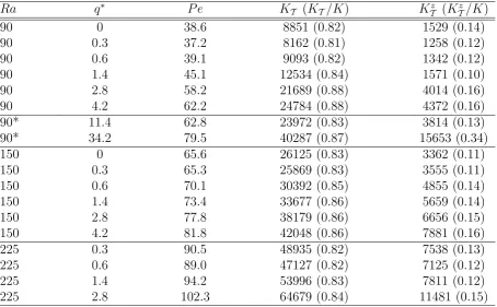
Table 1: Convection simulations used in this work. All simulations use P r = 1 and E = 10−5
. Ra is the Rayleigh number based on the average boundary heat-flux. All models employ a Y1
1 inner boundary condition and a spherically symmetric outer boundary condition except those denoted with an asterisk, which employ a Y1
1 outer boundary condition and a spherically symmetric inner boundary condition. Velocity is measured in units of the P´eclet number,P e=U d/κ=p
Figure 1: a) kinetic energy plotted against time for different values ofq∗ (top). Time is measured in units ofd2
/κ. b) and c) kinetic energy as a function of harmonic degreel and order mplotted up to degree and orderl=m= 30 at timet= 11 in a) (solid lines) and averaged over the period of time shown in a) (dashed lines). Other parameter values areE= 10−5
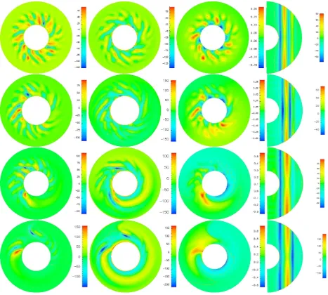
[image:18.595.161.431.104.656.2]Figure 2: Snapshots of simulations att= 11 in Figure 1a. From top to bottom: models withq∗= 0, 0.6, 1.4 and 4.2. Other parameter values areE = 10−5
, P r= 1,Ra = 90. From left to right: ur in the equatorial plane;uφin the equatorial plane; temperature perturbation with the spherically symmetric (Y0
Figure 3: Snapshots of the azimuthal component of the zonal flow, uz
φ, for q∗ = 1.4 (left) and q∗ = 4.2 (middle). Snapshots of the vertically (z) averaged azimuthal component of the zonal flow, [u]z
φ, as a function of radius for various values of q∗ (right). Snapshots are taken at t = 11 in Figure 1a. Other parameter values areE= 10−5
,P r= 1, Ra= 90.
Figure 4: Snapshots, taken att= 11 in Figure 1a, of the θ (top) andφ(bottom) components of equation (11) for a model withE = 10−5
,P r= 1,Ra= 90, q∗= 4.2 and a Y1
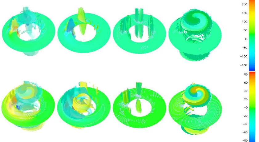
[image:20.595.89.510.371.602.2]Figure 5: Snapshots of the azimuthal component of the nonzonal (m6= 0) flow,unz
φ , atφ= 180◦(left), 225◦, 270◦ and 315◦ (right) forq∗= 4.2. Snapshots are taken att= 11 in Figure 1a. Other parameter values are
E= 10−5
,P r= 1,Ra= 90.
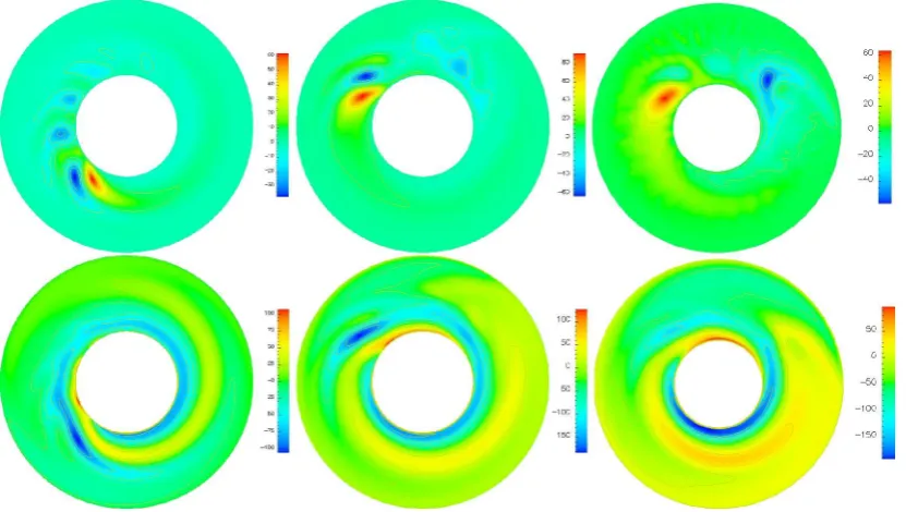
Figure 6: Time-averaged flows for E = 10−5
, P r = 1 and q∗ = 1.4. ur (top) and uφ (bottom) in the equatorial plane forRa= 90 (left), 150 (middle), and 225 (right). Time-averages span 6 time units, which are measured in units ofd2
[image:21.595.92.508.401.636.2]Figure 7: Snapshots of ur (left) and uφ (right) in the equatorial plane forRa = 90 andq∗ = 34.2 with a
Y1
1 outer boundary condition. φ= 0◦ corresponds to the rightmost edge of the plots and is the longitude of minimum heat-flux; maximum heat-flux is imposed atφ= 180◦. Other parameter values are E= 10−5
, P r= 1,Ra= 90.
Figure 8: Snapshots of theφcomponent of the thermal wind balance (first two terms in equation (11)) for a model withE = 10−5
, P r = 1, Ra= 90 and q∗ = 34.2 with aY1
[image:22.595.91.509.417.616.2]Figure 9: Snapshots (left) and time-averages (right) ofuφ in Mollweide projection forRa= 90 andq∗= 0.3 (top),Ra= 90 andq∗= 1.4 (middle) andRa= 225 andq∗= 1.4 (bottom). Snapshots are taken att= 11 of Figure 1a. Time-averages span 6 time units, which are measured in units ofd2