This is a repository copy of Robust control of uncertain multi-inventory systems via Linear Matrix Inequality.
White Rose Research Online URL for this paper: http://eprints.whiterose.ac.uk/89762/
Version: Accepted Version
Article:
Bauso, D., Giarré, L. and Pesenti, R. (2010) Robust control of uncertain multi-inventory systems via Linear Matrix Inequality. International Journal of Control, 83 (8). pp.
1727-1740. ISSN 0020-7179
https://doi.org/10.1080/00207179.2010.491131
[email protected] https://eprints.whiterose.ac.uk/ Reuse
Unless indicated otherwise, fulltext items are protected by copyright with all rights reserved. The copyright exception in section 29 of the Copyright, Designs and Patents Act 1988 allows the making of a single copy solely for the purpose of non-commercial research or private study within the limits of fair dealing. The publisher or other rights-holder may allow further reproduction and re-use of this version - refer to the White Rose Research Online record for this item. Where records identify the publisher as the copyright holder, users can verify any specific terms of use on the publisher’s website.
Takedown
If you consider content in White Rose Research Online to be in breach of UK law, please notify us by
arXiv:0710.4765v1 [math.OC] 25 Oct 2007
Robust control of uncertain multi-inventory
systems via Linear Matrix Inequality
D. Bauso,
aL. Giarr´e
band R. Pesenti
c,1a Dipartimento di Ingegneria Informatica
Universit`a di Palermo, Viale Delle Scienze, 90128 Palermo, Italy.
b Dipartimento di Ingegneria dell’Automazione e dei Sistemi
Universit`a di Palermo, Viale Delle Scienze, 90128 Palermo, Italy.
cDipartimento di Matematica Applicata - Universit`a “Ca’ Foscari” di Venezia,
Dorsoduro 3825/e, 30123 Venezia, Italy.
Abstract
We consider a continuous time linear multi–inventory system with unknown de-mands bounded within ellipsoids and controls bounded within ellipsoids or poly-topes. We address the problem ofε-stabilizing the inventory since this implies some
reduction of the inventory costs. The main results are certain conditions under which ε-stabilizability is possible through a saturated linear state feedback control.
All the results are based on a Linear Matrix Inequalities (LMIs) approach and on some recent techniques for the modeling and analysis of polytopic systems with saturations.
Key words: Impulse Control, Inventory Control, Hybrid Systems
1 Introduction
We consider a continuous time linear multi–inventory system with unknown demands bounded within ellipsoids and controls bounded within ellipsoids or polytopes. The system is modelled as a first order one integrating the discrepancy between controls and demands at different sites (buffers). Thus, the state represents the buffer levels. We wish to study conditions under
1 Corresponding author R. Pesenti, Research supported by PRIN “Advanced control and
which the state can be driven within an a-priori chosen target set through a saturated linear
state feedback control. Let ε be a maximal dimension of the target set, the above problem
corresponds to ε-stabilizing the state.
Motivations forε-stabilizing the state derive from the benefits associated to keeping the state
and consequently also the inventory costs bounded. This work is in line with some recent literature on robust optimization [1,5] and control [2] of inventory systems. Here as well as in [2] we focus on saturated linear state feedback controls since such controls arise naturally in any system with bounded controls.
The main results of this work can be summarized as follows. Initially we introduce the
necessary and sufficient conditions for theε-stabilizability in the form of an inclusion between
convex sets. In the case where both demands and controls are bounded within polytopes, it is well known that verifying such conditions is NP-hard [10]. Here, we prove that verification becomes easy when both demands and controls are bounded within ellipsoids (we will refer
to it as the ellipsoidal case). This is possible by rewriting the inclusion between ellipsoids in
terms of unconstrained quadratic maximization.
For the ellipsoidal case, we first characterize invariant sets through a fourth degree condition. As verifying such a condition is difficult, we then propose the best quadratic approximation of the same condition. We proceed by describing the region of linearity of the control and conclude by providing LMI conditions on the target set under which the saturated control
ε-stabilizes the system. The case where demands are bounded within ellipsoids and controls
are bounded within polytopes (we will refer to it as the polytopic case) is an open problem
and we propose certain sufficient LMI conditions to solve it.
All the results are based on a Linear Matrix Inequalities (LMIs) approach in line with the recent work [6] on inventory/manufacturing systems. In particular, when addressing the poli-topic case, we use the same technique provided in [9] to rewrite the model with saturations in polytopic form. Once we do this, we can apply the LMI analysis covered in the book [7] for polytopic systems.
This paper is arranged as follows. In Section 2, we formulate the problem. In Section 3, we introduce necessary and sufficient conditions for the admissibility of the problem. In Sections 4 and 5 we study the problem with ellipsoidal and polytopic constraints respectively. Finally, in Section 6, we draw some conclusions.
2 Problem Formulation
Consider the continuous time linear multi–inventory system
˙
u
1u2
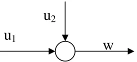
[image:4.612.231.368.57.119.2]w
Fig. 1. Graph with one node and two arcs.
where x(t) ∈ IRn is a vector whose components are the buffer levels, u(t) ∈ IRm is the
controlled flow vector, B ∈ Qn×m, with m ≥ n and rank(B) = n is the controlled process
matrix andw(t)∈IRnis the unknown demand. To model backlogx(t) may be less than zero.
Demands are bounded within ellipsoids, i.e.,
w(t)∈ W ={w∈Rn :wTRww≤1}. (2)
In a first case, in the following referred as ellipsoidal case, controls are bounded within
ellipsoids,
u(t)∈ U ={u∈Rm :uTRuu≤1}. (3)
In a second case, in the following referred as polytopic case, controls are bounded within
polytopes
u(t)∈ U ={u∈Rm : u− ≤u≤u+
} (4)
with assigned u+, u−.
For any positive definite matrix P ∈ Rn×n, define the function V(x) = xTP x and the
ellipsoidal target set Π = {x ∈ IRn : V(x) ≤ 1}. In addition, for any matrix K ∈ Rn×n,
define as saturated linear state feedback control any policy
u=−sat{Kx}=
−Kx if Kx∈ U
u(x)∈∂U otherwise (5)
where hereafter ∂F indicates the frontier of a given set F.
Problem 1 (ε-stabilizing) Consider a system (1) in the ellipsoidal or polytopic case. Find conditions on the positive definite matrix P ∈ Rn×n, under which there exists a saturated linear state feedback control u = −sat{Kx} such that it is possible to drive the state x(t)
within the target set Π.
Solving the above problem corresponds to ε-stabilizing the state x within Π.
Example 1 Throughout this paper we consider, as illustrative example, the graph with one node and two arcs depicted in Fig. 1. The incidence matrix is B = [1 1]. The continuous time dynamics is
˙
x(t) = [1 1]
| {z }
B
u1(t)
u2(t)
| {z }
u
−w =u1(t) +u2(t)−w(t),
with demand bounded in the ellipsoid
and with the following either ellipsoidal or polytopic constraints on the control u
(u1+u2)2 ≤1, (6)
−2≤u1 ≤3, −2≤u2 ≤1. (7)
Finally, the target set is the sphere of unitary radius Π ={x∈R:x2 ≤1}.
3 Stability necessary and sufficient conditions
System (1) is ε-stabilizable if and only if for all w ∈ W, there exists u ∈ int{U} such that
Bu=w (see, e.g., [3]). For the short of notation, the previous condition is usually expressed
as
BU ⊃ W. (8)
Deciding whether (8) holds is NP-hard, when U and W are polytopes. Here, we prove that
verifying (8) becomes easy when both U and W are ellipsoids. Observe that we can rewrite
Bu = w as uB = B−1w− B−1Nu
N, where B = [B|N] being B a basis of B and N the
remaining columns of B, correspondingly uB are the n components of u associated to the
basis B and uN are the m−n components of u associated to the columns in N.
As we observe that (8) is equivalent to
max
w∈Wu∈Rminm
:Bu=wuRuu <1,
Condition (8) holds if and only if
max
w∈WuNmin∈Rm−n
f(uB(w, uN), uN) =
=hwTB−T
−uTNNTB−T
|uTNiRu
B−1w− B−1Nu
N
uN
<1 (9)
When we consider the illustrative example in Section 1, we have B = [1], N = [1] then
problem (9) becomes
max
−1≤w≤1umin2∈R
f(uB(w, u2), u2) =
= [w−u2|u2]
1 0 0 1
w−u2
u2
= (w−u2)2+u22 <1 (10)
Now consider, functionf(uB(w, uN), uN). It is a differentiable convex function inuN. Then, for
anyw∈ Wwe can analytically determine the best responseu∗
by imposing
∇uNf(uB(w, uN), uN) = 2
h
−NTB−T
|IiRu
B−1w− B−1Nu
N
uN
= 0,
where I is the (m−n)×(m−n) identical matrix. We obtain
u∗N(w) =−
h
−NTB−T|IiRu
−B−1N
I −1
−NTB−T|I
Ru
B−1
0
| {z }
M
w=−Mw,
where 0 is the (m−n)×n null matrix. In the example under consideration, we have
u∗2(w) =−
[−1|1]
1 0 0 1 −1 1 −1
[−1|1]
1 0 0 1 1 0 w=
w
2.
For any w∈ W the minimal value off(uB(w, uN), uN) is
f(uB(w, u∗
N(w)), u∗N(w)) =w∗TΦw∗,
where
Φ = [B−T +MTNT
B−T
| −MT]
| {z }
HT
Ru
B−1+B−1NM −M
| {z }
H
=HTRuH (11)
is a positive definite n×n matrix, asM is full rank. So far, we have shown that we can find
the optimal value of problem (9) by solving problem
max
w∈W =w
TΦw, (12)
and checking that the optimal value is less than one.
We are ready to observe that problem (12) is easy as it reduces to determining the eigenvectors
of ann×n matrix.
Theorem 1 System (1) is ε-stabilizable if and only if w∗TΦw∗ < 1, for all w∗ eigenvec-tors associated to the maximum eigenvalue of matrix R−1
w Φ whose weighted quadratic norm
w∗TR
ww∗ is equal to 1.
Proof. AswTΦwis convex, its optimal valuew∗ lays on the frontier∂W of the setW, i.e., for
w∗TR
ww∗ = 1. Imposing the Karush Kuhn Tucker first order optimality condition, we obtain
2(Φ−λRw)w∗ = 0. Then the optimal values ofw∗ are some of the matrixRw−1Φ eigenvectors
whose weighted quadratic normw∗TR
ww∗ is equal to 1. In particular,w∗ are the eigenvectors
associated to the maximal eigenvalues of R−1
In the example under consideration Φ =h1
2
i
and w∗ =±1 then w∗TΦw∗ = 1
2 <1, hence the
associated system is ε-stabilizable.
In the following we discuss for which initial state the system is certainlyε-stabilizable through
a (pure) linear state feedback control; hence we show that if we saturated the previous linear
policy the system is ε-stabilizable for any initial state.
4 Ellipsoidal constraints
Let us start by considering only the constraints (2) on w and neglect the ellipsoidal
con-straints (3) onu. Among the saturated linear state feedback control (5) we prove that we can
solve Problem 1 using controls of type u=sat{−kHx}, with k ∈R and H ∈Rn as defined
in (11). Note that matrixH is a right inverse of B, that is BH =I. We motivate the choice
ofu=−sat{kHx} withH as defined in (11) as such a control describes the best response of
uunder the worst w as proved in the previous section. Also, note that the scalark ∈Rmust
be lower than a certain value, which means that we cannot use a bang-bang control. This is
motivated by the following reason. If we use a control u = sat{−kHx}, then the necessary
and sufficient condition (8) becomes
BUlin⊃ W (13)
where
Ulin ={u∈Rm : u=−kHx, k2xTHTRuHx≤1}.
Following the derivation of (12) in the previous Section, we have that (13) holds if and only if
k2w∗TΦw∗ <1.
For k = 1 the above condition holds true as it reduces to (12). Obviously, the value ˆk =
q
1
w∗TΦw∗ is an upper bound for k, namely, we must choose k such thatk < ˆk if we wish the
necessary and sufficient condition (13) be satisfied.
With the above considerations in mind, we can conclude that the dimensions of the target Π where it is possible to drive the state are lower bounded.
Denote by λmax(Z) the maximum eigenvalue of a given matrix Z. In the following theorem
we prove that ˙V(x) <0 within a given set (invariant set). This result will allow exploiting
V(x) as a Lyapunov function to prove the convergence to the target set Π.
Theorem 2 Consider system (1) subject to the only ellipsoidal constraints (2) on w, and controlled via linear state feedback u = −kHx, with H such that BH = I. Then condition
˙
V <0 holds if and only if
k2(xTP x)2−xTP R−1
Proof. For H such thatBH =I, condition ˙V <0 is equivalent to
2kxTP x+ 2wTP x > 0. (15)
We aim at proving that ˙V < 0 holds for any x external to an appropriate smooth closed
surface. To do this, we look for an x∈ Rn inducing a solution strictly greater than zero for
the following problem
min
w∈Wζ(x, w) = 2kx
TP x+ 2wTP x. (16)
Asζ(x, w) is linear inw, the optimalw∗ must lay on the boundary of setW. The Karush Kuhn
Tucker conditions impose thatP x=−λRww∗ for someλ≥0, that isw∗ =−λ1R−w1P x. Note
that beingP full rank, it necessarily holts thatλ6= 0 for allx6= 0. Then,ζ(x, w∗) = 2kxTP x−
2
λx
TP R−1
w P x > 0. As w∗ lays on the boundary of W, we have w∗TRww∗ = x
T
P R−1
w P x
λ2 = 1
from whichλ =qxTP R−1
w P x. Hence,ζ(x, w∗)>0, and therefore also (15) holds, if and only
if (14) holds.
We now exploit V(x) =xTP xas a Lyapunov function to prove the convergence to the target
set Π. We determine under which conditions onP andk we have that ˙V <0 or, equivalently,
inequality (14) hold for any x6∈Π.
When P = νRw, (14) becomes k2xTP x > ν. Then, in this case, we can use V(x) to prove
the convergence of the system to Π for k2 ≥ν.
In the following, we consider the general case when P 6=νRw.
Lemma 1 Consider system (1) subject to the only ellipsoidal constraints (2) on w, and controlled via linear state feedbacku=−kHx, with H such thatBH =I. Then,k2(xTP x)2−
xTP R−1
w P x > 0holds for anyx6∈Πif and only if k2−xTP R−w1P x≥0holds for anyx∈∂Π. Proof. (Necessity). Assume that there exists ˆx ∈∂Π such that k2 −xTP R−1
w P x < 0. Then,
there also exists a ball Ball(ˆx, r) centered in ˆx with a sufficiently small radius r > 0 such
that for all x∈Ball(ˆx, r) we have k2−xTP R−1
w P x < 0. This implies that there exist x6∈Π
for which condition (14) does not hold.
(Sufficiency). Assume that k2 −xTP R−1
w P x ≥ 0 holds for any x ∈ ∂Π. By contradiction,
consider ˆx 6∈ Π, i.e., ˆxTPxˆ = ρ > 1, such that k2(ˆxTPxˆ)2 − xˆTP R−1
w Px <ˆ 0, that is
k2ρ2−xˆTP R−1
w Px <ˆ 0. Then, there exists ˜x = √xˆρ ∈ ∂Π such that k
2ρ2−ρx˜TP R−1
w Px <˜ 0,
that is k2ρ−x˜TP R−1
w Px <˜ 0. This latter result is contradictory as we cannot have k2ρ <
˜
xTP R−1
w Px˜≤k2, forρ >1.
Lemma 2 Consider system (1) subject to the only ellipsoidal constraints (2) on w, and controlled via linear state feedback u=−kHx, with H such that BH =I. We can use V(x)
to prove the convergence of the system to Π for k2 ≥λ
max(R−w1P). Proof. Condition k2 −xTP R−1
xTP R−1
w P x} ≥ 0. Imposing the Karush Kuhn Tucker first order optimality condition, we
obtain 2(P R−1
w P −λP)x∗ = 0. Then the optimal values of x∗ are some of the matrix R−w1P
eigenvectors whose weighted quadratic norm x∗TP x∗ is equal to 1. In particular, x∗ are
the eigenvectors associated to the maximal eigenvalues of R−1
w P. For vectors x∗, condition
k2−x∗TP R−1
w P x∗ ≥0 becomes k2−λmax(R−w1P)x∗TP x∗ ≥0, that is k2−λmax(Rw−1P)≥0.
Observe that the system converges to the target set ΠR={x:k2xTRwx≤1}as any feasible
target set Π = {x : xTP x ≤ 1}, with k2 ≥ λ
max(R−w1P) includes ΠR. Indeed, Π ⊇ ΠR if
xTP x−k2xTR
wx=xT(P −k2Rw)x≤0 or equivalently if P −k2Rw 0. In turn, the latter
condition is equivalent to R−1
w P −k2I 0 that certainly holds as k2 ≥λmax(R−w1P)
In the next theorem we introduce the constraints on controls (3). To this end, we need to
define the family of ellipsoid Σ0(ξ) = {x∈ Rn : xTP x≤ x(0)TP x(0) := ξ} parametrized in
ξ ≥1.
Theorem 3 Given system (1) in the ellipsoidal case, we can drive the state x(t) from any initial value x(0) ∈ Σ0(ξ) to the target set Π via linear state feedback u = −kHx if the
following conditions hold
k2 ≥λmax(R−w1P) (17)
k2ξλmax(P−1Φ)≤1. (18)
Proof. By Lemma 2, under condition (17) it holds ˙V(t) <0 for all x(t) 6∈ Π and then V(x) can be considered as a Lyapunov function for the convergence of the state to the set Π when
the linear control u=−kHx is implemented. Condition ˙V(t)<0 also implies that Σ0(ξ) is
invariant with respect to the same linear feedback asξ ≥1 which means Σ0(ξ)⊇Π. Then
max
t≥0 u
T(t)R
uu(t)≤ max x∈Σ0(ξ)k
2xTHTR
uHx= max
x∈Σ0(ξ)k
2xTΦx=k2ξλ
max(P−1Φ).
Therefore the constraint u=−kHx(t) ∈ U for all t ≥0 is enforced if (18) holds true.
The following theorem provides a solution to Problem 1. Let us denote byX the set of states
x where we can define a linear control u(x) = −kHx, i.e., X = {x: −kHx∈ U}. Consider
the saturated linear state feedback control of type
u(x) =
−kHx if x∈X
−√ Hx
xTHTR uHx
if x6∈X . (19)
Theorem 4 Consider a system (1) in the ellipsoidal case. For any positive definite matrix
P ∈Rn×n satisfying condition (17), the saturated linear state feedback control (19) drives the state x(t) within the target set Π for any initial state x(0).
Proof. By construction,u(x) is a continuous function with U as codmain. When we use such
a control, we know that ˙V(x)<0 also holds for any x6∈Π, if Π⊂X and k2 ≥λ
(see Lemma 2).
First observe that, for all x ∈ ∂X, we have xTP x > k2xTHTR
uHx = 1, where the
lat-ter inequality holds as Π ⊂ X. Then, for any x 6∈ X, that is for k2xTHTR
uHx > 1, we
have xT
P x xTHTR
uHx > k
2 ≥ λ
max(R−1P) since both xTP x and xTHTRuHx are positive definite
quadratic forms.
In Lemma 2, we have proved that ˙V(x) < 0 for x ∈ X\Π. Now, we consider x 6∈ X. We
have ˙V(x)<0 if and only if−xTP Bu(x) +xTP w >0, for allw∈ W, that is
min
w∈W
(
xTP x
√
xTHTR uHx
+xTP w
)
>0 (20)
must hold. Applying the Karush-Kuhn-Tuker conditions, we transform (20) in √ xTP x
xTHTR uHx−
q
xTPTR−1
w P x > 0. In turn, the latter inequality holds if x
T
P x xTHTR
uHx −λmax(R
−1P) > 0, as
xTPTR−1
w P x≤λmax(R−1P)xTP x. We then conclude that ˙V(x)<0 since x
T
P x xT
HT
RuHx > k
2 ≥
λmax(R−1P).
Observe that the saturated linear state feedback control (19) is not decentralized in the sense
that the generic ith control ui in general depends on the demand at different nodes and on
the other controls uj, j 6=i. This is due to either the structure of matrixH or the ellipsoidal
constraints (3).
Remark 1 Consider the two equivalent matrix inequalities on P and Q=P−1,
(2k−1)P −P R−1
w P ≥0, (2k−1)Q−R−w1 ≤0. (21) Trivially, any P satisfying condition (17) also satisfies the two above matrix inequalities.
Matrix inequalities of the above form will be used in the following sections.
Example 2 Consider the graph depicted in Fig. 1, with one node and two arcs and incidence matrix B = [1 1]. Controls are subject to ellipsoidal constraints (6). Then we have,Rw = 1,
Ru =I and Φ = 12. We can stabilize the system within Π ={x∈R :x2 ≤1} for any initial state x(0) ≤ √2 via a pure linear state feedback u = −kHx. To see this take Q = I, and observe that the matrix inequality on Q (21) is satisfied for any k ≥ 1. Furthermore, if we assume k = 1, then from (18) we must have k2 = 1 ≤ 2
ξ2 = 2
x(0)2.
5 Polytopic constraints
Controls u are subject to the polytopic constraints (4). Again, we study under which
such that BH = I. In this case, we interpret the sat{.} operator as componentwise. More specifically, we choose the control
ui =sat[u−
i,u
+
i]{−kHi•x}, (22)
with H such thatBH =I, Hi• denoting theith row of H and where, for any given scalar a
and b
sat[a,b]{ζ}=
b, if ζ > b, ζ, if a≤ζ ≤b, a, if ζ < a.
Henceforth we omit the indices of the satfunction.
Under the controlu=sat{−kHx}, the closed loop dynamics becomes
˙
x=Bsat{−kHx} −w. (23)
Our idea is to rewrite the above dynamics in the following polytopic form
˙
x=A(t)x(t)−w(t), w(t)TRww(t)≤1, (24)
where the time varying matrices A(t) are expressed as convex combinations of 2m matrices
Aj, j = 1, . . . ,2m. More precisely the expressions for A(t) are
A(t) =
2m
X
j=1
σj(t)Aj,
2m
X
j=1
σj(t) = 1. (25)
The procedure to compute matrices Aj’s is borrowed from [9] and recalled below. Let us
rewrite the control policy as
ui =sat{−kHi•x}=θi(x)(−kHi•x),
where θi(x) are the “degree of saturation” of the control components defined as follows
θi(x) =
u−
i
−kHi•x if −kHi•x < u
−
i
1 if u−
i ≤ −kHi•x≤u+i u+i
−kHi•x if −kHi•x > u
+
. (26)
Letθ = [θ1, . . . , θm] be a vector whose componentsθi are such that 0≤θi ≤1 and represent
lower bounds of θi(x(t)), for t ≥ 0. Lower bounds depend on x(0) and can be computed
as θi = minx∈Σ0(ξ)θi(x) where we remind the definition of Σ0(ξ) = {x ∈ Rn : xTP x ≤
x(0)TP x(0) :=ξ}. Also define the vector ψθ = [ψθ
1, . . . , ψmθ] with ψiθ = θ1i and the associated
portion of the state space
According to the above definition of the θis we derive that S(ψθ)⊇Σ0(ξ). Note that we can
affirm thatθi are lower bounds because the state trajectory never exitsS(ψθ) as we will show
in the proof of Theorem 5.
Consider now the 2m vectorsγ
j ∈ {1, θ1} ×. . .× {1, θm}, with j = 1, . . . ,2m. In other words,
γj is anm component vector withith component γji taking value 1 orθi. Then, each matrix
Aj can be expressed as Aj = −Bkdiag(γj)H. Roughly speaking each vector γj stores the
minimum and or maximum degree of saturation of all control components. Also, note that
matrices Ajs induce a partition of S(ψθ) into regions Xj, with j = 1. . . ,2m. Each region is
defined as the set of state values such that the control components are saturated with degree
of saturation equal to γji, namely
Xj ={x∈Rn: θi(x) =γji, i= 1, . . . , m}.
We remind here that γji is the ith component of γj.
To complete the derivation of the polytopic form (24) it is left to be noted that given any
x(t) ∈ S(ψθ) we can compute the associated degree of saturation from (26) and derive the
weights σj(t) of the convex combination (25). All the results in the rest of this section try to
give an answer to Problem 1 with respect to the polytopic system (24). For each Aj, let us
define a matrix
Mj =QATj +AjQ+αQ+
1
αR
−1
w
for a given positive and arbitrarily chosen scalarα and let (λr
j, vjr) withr∈ {1, . . . , n}be the
negative eigenvalues and corresponding eigenvectors of Mj.
Theorem 5 Consider system (1) in the polytopic case. The saturated linear state feedback control (22) drives the state x(t) within the target set Π if
Xj ⊆Span{vjr}, for all j = 1, . . . ,2n. (27)
Proof. First of all, note that if (27) holds true then Σ0(ξ) is invariant. Consequently, as
Σ0(ξ) ⊆ S(ψθ) and by definition x(0) ∈ Σ0(ξ), we also have that the state trajectory x(t)
will never exit S(ψθ). Now, we must show that ˙V(x) < 0 for all x and w such that x 6∈ Π,
u∈ U and w∈ W. In formulas, we must have
˙
V(x) = ˙xTP x+xTPx˙ = [A(t)x−w]TP x+xTP[A(t)x−w] =
= xTA(t)TP x+xTP A(t)x−wTP x−xTP w < 0 (28)
for all x and w satisfying
1−xTP x≤0 (29)
wTRww−1≤0. (30)
there exist α, β ≥0, such that for all x and w x w T
A(t)TP +P A(t)T +αP −P
−P −βRw
x w
−α+β≤0. (31)
Trivially it must hold β ≤α. Assume without loss of generality β =α. Remind that α and
β can be chosen arbitrarily. After pre and post-multiplying byQ=P−1, the above condition
becomes x w T
QA(t)T +A(t)TQ+αQ −I
−I −αRw
x w
≤0. (32)
Now, as the state never leaves the region S(ψθ), i.e., x(t) ∈ S(ψθ), we can always express
A(t) as convex combination of the Ajs as in (25).
By convexity, the above condition is true if it holds, for all j = 1, . . . ,2n,
x(j)
w(s)
T QAT
j +ATjQ+αQ −I
−I −αRw
x(j)
w(s)
≤0. (33)
Using the Shur complement the condition (33) is implied by (27).
Stronger conditions are established in the following theorem which also highlights the
depen-dence of Mj on the scalar α.
Theorem 6 Consider system (1) in the polytopic case. The saturated linear state feedback control (22) drives the state x(t) within the target set Π if there exists a scalar α ≥ 0 such that
Mj <0, for all j = 1, . . . ,2n. (34)
Proof. Trivially, if we observe that (34) implies (27).
Both (27) and (34) are sufficient, but not necessary, conditions. When they hold, we are sure that the system state converge to a state strictly included in the target set Π. We discuss more on this topic in the next section.
5.1 Approximation error
We wish to estimate the difference in terms of volumes between the target set Π and the target
On this purpose, denote by Qj the matrix of the smallest (in volume) ellipsoid satisfying
Mj <0, which is given by
Qj = arg inf
Q minα {det(Q), Mj =QA T
j +AjQ+αQ+
1
αR
−1
w <0}. (35)
To do this, let matrix A be the matrix Aj withj = 1, . . . ,2m obtained when no controls are
saturated and note that the dynamics associated to this single matrix is the same as if we
assumed the controls unbounded. To be more precise, A = −BkH as all components of γj
are equal to one. Remind that γj stores the degree of saturation of each control component.
Also let us define Q the solution of (35) for Aj =A. We do this, as the target set Π within
which we can stabilize the state, must inscribe the ellipsoid defined by Q, i.e.,
Π⊃ {x∈Rn: xTQ−1x≤1}.
Similarly, let matrixAbe the matrixAj withj = 1, . . . ,2m obtained when all controls are
sat-urated at their lowest degree of saturation. To be more precise, A=−Bkdiag([θ1, . . . , θm])H
as all components of γj are equal to θi for i = 1, . . . , m. If we also define Q the solution
of (35) forAj =A, the target set Π must be inscribed in the ellipsoid defined by Q, namely,
Π⊂ {x∈Rn: xTQ−1x≤1}.
The approximation error can be measured by the ratio
e= det(Q
−1
)−det(Q−1)
det(Q−1) .
Example 3 Consider the graph depicted in Fig. 1, with one node and two arcs, incidence matrix B = [1 1], and target set Π = {x ∈ R : x2 ≤ 1}. Controls are subject to polytopic
constraints (7). Take H = [1 2
1 2]
T and k = 1. Then according to (26) we have (here x is a scalar)
θ1(x) =
2
x/2 if x/2>2
1 if −3≤x/2≤2
− 3
x/2 if x/2<−3
θ2(x) =
2
x/2 if x/2>2
1 if −1≤x/2≤2
− 1
x/2 if x/2<−1
.
If we consider initial states x(0) satisfying −10 ≤ x(0)≤ 10, possible lower bounds for the
θ’s are θ1 = 25 and θ2 = 15. Note that S(ψθ) = {x ∈ Rn : −10 ≤ x ≤ 10}. Vectors γ’s and
matrices A’s turn out to be
γ1 = [1 1]T γ2 = [0.4 1]T γ3 = [1 0.2]T γ4 = [0.4 0.2]T
A1 =−2 A2 =−1.4 A3 =−1.2 A4 =−0.6
. (36)
Dynamics (24) is then
˙
with P4
j=1σj(t) = 1. Furthermore, we have
M1 = [−4 +α]Q+ α1 M2 = [−2.8 +α]Q+ 1α
M3 = [−2.4 +α]Q+ 1α M4 = [−1.2 +α]Q+ 1α
.
To apply Theorem 5 and 6, note that A =A4 and that M4 <0 implies consequently Mj <0 for allj. The solution of (35), forj = 4isQ4 =Q= 0.136 andα= 0.6, then the approximation
error is e = 1−0.36
0.36 = 1.78.
6 Conclusions and future works
We have addressed the problem of ε-stabilizing the inventory of a continuous time
lin-ear multi–inventory system with unknown demands bounded within ellipsoids and controls bounded within ellipsoids or polytopes. Motivations are due to the cost reduction associated with a bounded inventory. As main results we have provided certain LMIs conditions under
which ε-stabilizability is possible through a saturated linear state feedback control. We have
also exploited some recent techniques for the modeling and analysis of polytopic systems with saturations.
This work is a continuation of [2] and is in line with some recent applications of LMI tech-niques to inventory/manufacturing systems [6]. In a future work, we will study the validity in probability of the LMI conditions derived in this paper. This is in accordance with some
recent literature onchance LMI constraints developed in the area of robust optimization [4,8].
References
[1] E. Adida, and G. Perakis, “A Robust Optimization Approach to Dynamic Pricing and Inventory Control with no Backorders”,Mathematical Programming, Ser. B vol. 107, 2006, pp. 97–129.
[2] D. Bauso, F. Blanchini, R. Pesenti, “Robust control policies for multi-inventory systems with average flow constraints”, Automatica, Special Issue on Optimal Control Applications to Management Sciences, vol. 42, no. 8, pp. 1255-1266, Aug. 2006.
[3] F. Blanchini, F. Rinaldi and W. Ukovich, “A network design problem for a distribution system with uncertain demands”,SIAM Journal on Optimization, 7 (1997), pp. 560–578.
[4] A. Ben-Tal, A. Nemirovsky, “On tractable approximations of uncertain linear matrix inequalities affected by interval uncertainty”, SIAM Journal on Optimization, vol. 12, pp. 811–833, 2002.
[5] D. Bertsimas, A. Thiele, “A Robust Optimization Approach to Inventory Theory ”, Operations Research, vol. 54, no. 1, Jan-Feb 2006, pp. 150–168.
[7] S. Boyd, L. El Ghaoui, E. Feron, and V. Balakrishnan,Linear Matrix Inequalities in System and Control Theory, volume 15 ofStudies in Applied Mathematics, Society for Industrial and Applied Mathematics (SIAM), Philadelphia, PA, 1994.
[8] G. Calafiore, M. C. Campi, “Uncertain Convex Programs: Randomized Solutions and Confidence Levels”, Mathematical Programming, 102, pp. 25–46, 2005.
[9] J. M. Gomes da Silva, Jr. and S. Tarbouriech “Local Stabilization of Discrete-Time Linear Systems with Saturating Controls: An LMI-based Approach”, IEEE Trans. on Automatic Control, vol. 46, no. 1, pp. 119-124, Jan. 2001.
[10] S.T. McCormick, “Submodular containment is hard, even for networks”, Operations Research Letters, 19 (1996), pp. 95–99.