Addressing the Challenge of Defining Valid Proteomic Biomarkers and Classifiers

R E S E A R C H A R T I C L E

Open Access

Addressing the Challenge of Defining Valid

Proteomic Biomarkers and Classifiers

Mohammed Dakna

, Keith Harris

, Alexandros Kalousis

, Sebastien Carpentier

, Walter Kolch

, Joost P Schanstra

,

Marion Haubitz

, Antonia Vlahou

, Harald Mischak

, Mark Girolami

Abstract

Background:The purpose of this manuscript is to provide, based on an extensive analysis of a proteomic data set, suggestions for proper statistical analysis for the discovery of sets of clinically relevant biomarkers. As tractable example we define the measurable proteomic differences between apparently healthy adult males and females. We choose urine as body-fluid of interest and CE-MS, a thoroughly validated platform technology, allowing for routine analysis of a large number of samples. The second urine of the morning was collected from apparently healthy male and female volunteers (aged 21-40) in the course of the routine medical check-up before recruitment at the Hannover Medical School.

Results:We found that the Wilcoxon-test is best suited for the definition of potential biomarkers. Adjustment for multiple testing is necessary. Sample size estimation can be performed based on a small number of observations via resampling from pilot data. Machine learning algorithms appear ideally suited to generate classifiers.

Assessment of any results in an independent test-set is essential.

Conclusions:Valid proteomic biomarkers for diagnosis and prognosis only can be defined by applying proper statistical data mining procedures. In particular, a justification of the sample size should be part of the study design.

Background

The field of biomarker discovery or clinical proteomics has raised high hopes generated by reports on potential biomarkers, which in many cases subsequently could not be substantiated in validation studies [1,2]. Promi-nent examples are the findings in [3,4]. This develop-ment has resulted in large scepticism from both clinicians and regulatory agencies, which will make the application of valid biomarkers into the arsenal of clini-cal diagnostics even more of a challenge [5,6]. Further, it is now generally accepted that single biomarkers are unlikely to result in major advancements as the com-plexity of disease cannot be captured by a single marker; instead, a panel of such biomarkers must be employed [7,8]. However, it is equally evident that such a panel must consist of clearly defined and validated biomarkers in order to provide a well defined signature. This raises the issue of the definition of a valid biomarker. As this

is obviously of central importance, we have revisited this issue, not only employing theoretical considerations, but also by using a tractable yet realistic case study. The theoretical considerations in this area apply to the fol-lowing main challenges:

1 Is the change (frequency or abundance) of a cer-tain molecule observed in a proteomics study of dis-ease, the result of the disdis-ease, or does it merely reflect an artefact due to technical variability in the pre-analytical steps or in the analysis, biological variability, or bias introduced in the study (e.g. due to lifestyle, age, and gender)?

2 How should we estimate the number of samples required for the definition of likely valid biomarkers? 3 Which algorithms can be employed to combine biomarkers into a multi-marker classifier, and how can the validity of a multi-marker classifier be assessed? Is validation in an independent test set necessary?

* Correspondence: h.mischak@clinmed.gla.ac.uk

1_{Mosaiques diagnostics and therapeutics, Hannover, Germany}

Full list of author information is available at the end of the article

In an effort to investigate these issues and propose answers to these questions, we have employed different analysis and statistical strategies towards biomarker defi-nition and validation using a set of data obtained from real samples. While technical differences do exist between proteomics and peptidomics, these approaches investigate a highly similar chemical entity, and the pro-blems and challenges associated with the identification of potential proteomic and peptidomics biomarkers (fea-tures significantly associated with the studied physiologi-cal or pathophysiologiphysiologi-cal condition) are essentially identical. Therefore, we feel it is appropriate not to dis-tinguish between peptidomics and proteomics through-out this manuscript. Several platforms for proteomics or peptidomics are currently being used in biomarker dis-covery studies (reviewed in e.g. [9].

We have chosen data from CE-MS as one representa-tive example, due to the following reasons: a) CE-MS is being used in clinical trials and data from CE-MS are applied in clinical decision-making, b) sufficient datasets of CE-MS were available to us, and c) the analytical per-formance characteristics of the CE-MS platform are well documented [10,11]

In order to permit a rigorous and realistic assessment of the methodology, the study must (i) represent a real proteomic dataset that is acquired using the same tech-nologies and experimental design as for a biomarker study; (ii) be a classification problem with“typical” com-plexity, but simple enough to be tractable by standard methods; and (iii) permit the deployment of commonly used statistical analysis strategies in order to benchmark them against an unequivocal outcome. Based on these considerations we choose as an example the definition of proteomic differences between apparently healthy adult males and females. This avoids any bias due to a non-verifiable physiological condition in the subjects, since gender can be assessed with close to 100% confi-dence [12]. This design avoids an important problem in biomarker discovery pipelines: the so called verification bias. This bias occurs if subjects are not equally likely to have the diagnosis verified by a gold-standard test and if selection for further evaluation is dependent on the diagnostic test result. Of course, in general the clinical situation will not allow for such a sharp definition as in the male-female case, but standard methods exist for accounting for the verification bias if the clinical readout cannot be assigned with 100% confidence [13-15]. We also used a cohort of subjects with diabetes type II either with normal kidney function (controls, CD) or diabetic nephropathy (cases, DN) to demonstrate the applicability of the methods to a case where the clinical readout may not be verified with 100% confidence. The difference in the male-female study turned out to be more subtle than in the CD versus DN case, as the

differences between the proteomic profiles between males and females are less pronounced than in the CD-DN case.

As body fluid to be analysed we have chosen urine. The urinary proteome/peptidome is of high stability, reducing pre-analytical variability [16]. CE-MS was cho-sen as technology as it allows for the routine analysis of a large number of samples, and has been thoroughly validated as a platform technology for proteomic bio-marker studies [17]. As result of the current study we demonstrate the importance of a strict and correct use of statistics, especially adjustment for multiple testing. We further describe algorithms that enable prediction of the number of samples required for the definition of biomarkers with high confidence. The results presented here also show that different machine learning algo-rithms perform similarly (and very well) in establishing discriminatory multi-marker models. However, it is equally evident that these only lead to meaningful results if the number of data points employed is suffi-cient to learn the difference between the groups, and that the performance of such models can only be assessed on an independent test set. Although our results have been obtained with a particular proteomic technology, CE-MS, the principal conceptual considera-tions, and hence also the conclusions, are independent of the technology used. Therefore, the results reported here should also be applicable to other datasets gener-ated using alternative standard proteomics technologies such as LC-MS or MALDI. Unfortunately, to the best of our knowledge, there is currently no similar dataset publicly available for MALDI or for LC-MS. Hence, we cannot report on the application of the proposed meth-ods for either platform.

Results and Discussion Biomarker selection

at zero may either be biological, as the protein is really absent in these samples, or technical, as the protein is pre-sent but its signal is below the limit of detection (LOD) [18]. The only known fact about the point mass at zero is that those values are between zero and the LOD. In statis-tical terminology, the proteomics data are left censored. Therefore, usage of standard statistical methods which focus on one part of this mixture at a time can fail to detect differences between classes. The data employed here contains 1169 consonant differences (the group with the higher proportion of zeros has the smaller mean in the continuous component), 38 dissonant differences (the group with the higher proportion of zeros has a larger mean in the continuous component) and 9 without point-mass component. The higher number of consonant mar-kers reflects the fact that marmar-kers showing a higher mean are better detectable than those with a mean near to the LOD. A difference in means between the two groups may

have its origin in a difference in the proportion of zeros, a difference in the mean of the continuous component, or both. The standard parametrict-test may be inappropriate for such data as the underlying assumptions of the test are strongly violated. Non-parametric tests like the Wilcoxon rank sum test (WT) may be more appropriate [19], but may still fail to distinguish the contributions of the two mixture components to the male and female profiles [20]. This suggests the usage of hypothesis tests specifically developed for point-mass mixture data, like the two-part t-test, two-part WT and empirical likelihood ratio test, which tests the null hypothesis of no difference in the point-mass proportions and no difference in the means of the continuous components [20]. As expected, owing to differences in statistical power, the number of biomarkers declared statistically significant strongly varies with the type of test adopted (Table 1). When subsequently validat-ing in the hold-out set, the majority of the initially defined

CE-MS analysis

Healty male 21-40 years

Healty female 21-40 years

7

7

20

20

33

33

67

67

Evaluation of

individual biomarkers

Evaluation of

biomarker models

Figure 1Study design. Usage of samples and flow of information. 67 samples from males and females were each employed in a training set

potential biomarkers could not be confirmed. This result is likely due to the inherent multiplicity of the problem, strongly supporting the requirement for adjustment for multiple testing [21-23]. These results are even more pro-nounced when a smaller cohort is employed, resulting in≤ 10% of the potential biomarkers being confirmed in the test set (data not shown). To control the false discovery rate (FDR) as correction to multiple testing, the Benja-mini-Hochberg (BH) procedure was used [24]. In Table 1 we report the number of potential markers with adjusted

p-values less than 0.05. After adjustment for multiple test-ing, the WT reports the largest number of significant mar-kers (Table 1). Moreover, 78% of the 112 marmar-kers declared significant by the two-part WT are also significant when using the standard WT, indicating that using just standard WT, which is part of standard statistical software (e.g., SAS or SPSS), should enable definition of reliable biomar-kers. The fact that many of the values in the profiles are tied to zero only makes the WT conservative and thep -values more trustable [25]; as in a pilot study, a false

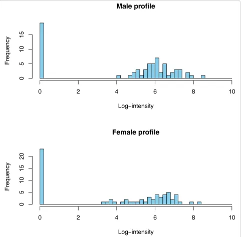
Male profile

Log

−

intensity

Frequency

0

2

4

6

8

10

0

5

10

15

Female profile

Log

−

intensity

Frequency

0

2

4

6

8

10

0

5

10

15

20

Figure 2Typical male and female peptide profiles. Distribution of a peptide included in the male-female comparative study. The frequency

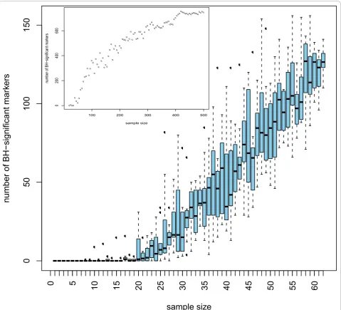
negative is less harmful than a false positive. To test the stability of the significant markers chosen by the different tests, we investigated which of the differentially expressed markers established will still be a valid marker when tested alone on an independent test set (2 × 67 samples). As seen from Table 1 the standard WT has the most markers holding up in the independent test set. Furthermore, the concordance between the biomarkers found in the training set and in the test set is only slightly lower than that for the two-part WT. The results given above argue in favour of using the standard WT for any similar proteomics data. Previous reports have already stressed that non-parametric statistical tests such as the WT may be more appropriate for proteomics data. However, the use of the standardt -test is still frequently used and reported in the literature [26-28]. We subsequently investigated the number of potential biomarkers that can be defined when employing only a subset of the original samples. Statistically, if a real difference exists, it may always be detected when the sam-ple size is ad-equate. Hence, studies on small cohorts may over-look important markers. With appropriate sample size all the differentially expressed markers should be detected. Of course, not every difference found with larger sample sizes will be of clinical relevance, hence the need for the incorporation of biological back-ground informa-tion. Interestingly, even a subset of the markers found using moderate sample size may still be enough for build-ing a good classifier. As expected, the number of signifi-cant markers increases with increasing sample size (see Figure 3). Our simulations, where populations of sizes up to 2 × 480 were generated using resampling with replace-ment from the 2 × 67 samples, showed that this behaviour stops at sample sizes around 2 × 400 where a plateau is reached (Figure 3 on top left). The concordance of these

potential biomarkers in the test set also increases with the sample size. With sample sizes less than 13, no differen-tially expressed markers are detected at all.

Resampling as means to define“better biomarkers” Variable selection may be seen as the first part in find-ing a good classifier and must be performed based on training data only. Usually, variable selection is per-formed only once using all the available training data. This may, however, introduce a substantial bias in declaring a biomarker differentially expressed. This fact is due to the biological variability in the compared populations (here male and female). Cross-validation and Monte Carlo cross-validation (random splitting into learning and test sets) may be adopted to protect the analysis against such a bias. However, as the number of biomarkers may be quite high, these procedures are computationally challenging. Holding out 30% randomly from the 134 male and female training samples and examining the distribution of these biomarkers in the 134 independent test samples, we can detect a clear advantage of the biomarkers that were found with higher frequency in the resamples. From Table 2 we see, provided enough resamplings are done (i.e.,N≥30), that if a biomarker is found significant in more than 75% of the independent resamples then the chance that it could be confirmed in the test set was between 70 and 100%. However, this procedure also results in a further reduc-tion of the available biomarkers, and appears to be only useful when a rather large number of potential biomar-kers should be reduced. In depth analysis of the data indicated that for building classifiers (see also below), a reduction via resampling of the number of biomarkers may not be necessary (data not shown). However, the

Table 1 The number of significant markers depends on the statistical test used

p-values Test No point-mass Dissonant Consonant Total Validated % Validated

unadjusted t-test 3 0 245 248 63 25%

Wilcoxon 4 5 314 323 109 33%

Two-part-t 3 8 229 240 68 28%

Two-part-W 4 11 286 301 104 34%

Empirical LRT 4 7 271 282 81 28%

BH-adjusted t-test 0 0 57 57 27 47.3%

Wilcoxon 3 1 137 141 58 41.1%

Two-part-t 0 3 66 69 30 43.4%

Two-part-W 3 6 103 112 55 49.1%

Empirical LRT 2 5 109 116 43 37.0%

implementation of such resampling is clearly advanta-geous for e.g. describing any association with (patho) physiology, as this procedure allows for identify-ing those biomarkers that show the highest likelihood of actually being associated with the investigated (patho) physiology.

Estimation of the sample sizes

An important question in the design of clinical proteomics studies is the selection of an appropriate sample size [29]. The number of units to be included in the study should typically address two issues. First, the differential sample

size Ndiff should allow the identification of putative

biomarkers that are differentially expressed between two conditions (e.g. disease versus control). Second, the discri-minative sample sizeNdiscof the training data should

allow the learning of a confident rule for classifying blinded items.

Estimation of the differential sample size

Here the question is: what is the minimum sample size required to attain a desired statistical power for detect-ing a meandetect-ingful difference between samples? This can

0

50

100

150

sample size

number of BH

−

significant mar

kers

0

5

₁₀

₁₅

₂₀

₂₅

₃₀

₃₅

₄₀

₄₅

₅₀

₅₅

₆₀

qqqq q

q q

q qq

q qq

q q

q q

q

q q

q q

q q

q

qqq q

q q

q q q

q q

q q

qqqqqq q

q qq

qq qq

q q

q qq

q qqq

qq q

qqqq qqqq

qqq qq

qqqqqqqqqqqqqqqqqqqq

100 200 300 400 500

0

200

400

600

sample size

number of BH

−

significant mar

kers

Figure 3Number of significant markers depends on sample size. From the 2 × 67 training data, data sets of sizesNdiffranging from 7 to 67

be answered by estimation of the differential sample size Ndiff. This sample size depends on the false positive rate

a, typically set at 0.05, the statistical power 1-b(e.g. 0.9) and the standardized effect size (e.g. Cohen’s δ) for quantifying how the classes differ. Indeed, the effect size and its variation turn out to be the most important fac-tors influencingNdiffestimation. Both, effect size and its

variation, are traditionally estimated from previously reported experimental data. Unfortunately, in proteo-mics typically no previous data are available and antici-pation of the expected as in [30,31] may hardly be justified. We therefore investigated a resampling-based approach by directly sampling from the pilot data at hand. To simulate a typical proteomics study, we ran-domly choose 7 samples of each gender from the total training set of 67 males and 67 females. From the 2 × 7 data, we used the bootstrap [32] to generate 2000 sam-ple sets of different larger sizes (2 × 10 to 2 × 120) without any assumption about the underlying distribu-tion of the sampled populadistribu-tion. To take into account the multivariate aspect of the problem, we ask for the sample size required for declaring all the markers signif-icant while controlling the FDR at 0.05 using the BH procedure. This is equivalent to conducting the single tests at a more stringent“average type one error” aave.

Using the result [24]

  



ave = − ave + − − ⎡

⎣

⎢ ⎤

⎦ ⎥

−

(1 ) 1 (1 ) ,

1

0 0

1

q q

where (1 -b)aveis the average power for a single

mar-ker (set e.g. to 0.9),q is the expected value of the false discovery rate, i.e.q = E(FDR), andπ0is the proportion

of markers that are differentially non expressed (true null). To estimate π0 we use the method described in

[33] and fit the observed distribution of the Wilcoxon p-values to the following two component model

f p( )=_{0 0}f p( )+ −(1 ₀)f_A( ),p

withf0(p) being the density of the null features (that is

the differentially non expressed markers) is given by the uniform distribution U(0, 1), whereasfA(p) is the

alter-native density for the differentially expressed markers. Hence we may write

f p( )=0+ −(1 0)fA( ).p

This resulted in a estimate π0 = 0.5652831 which

plugged into Equation 1 leads toaave= 0.00223.

To estimateNdiffwe set the value ofaave= 0.00223 to

control the FDR at 0.05 and examined for biomarkers that can be declared significantly differentially distribu-ted. WT was applied to each data set generadistribu-ted. Let  be the number of times the null hypothesis is rejected. Discarding 5% of  (the false positives) is essentially a power estimate. By examining the graphs as in Figure 4 the sample size required for any predefined power can be deduced. Obviously, the more precise the information about the effect size δ, the better the trial can be designed. If the sample size is“sufficiently large”, then the central limit theorem guarantees that δ will be approximately normally distributed. The bootstrap pro-vides a powerful tool to estimate the required differential sample size by directly sampling from the available data and has been shown to give an unbiased estimate of power [34]. However, the key issue here is that the avail-able data be reliavail-able and representative. In the absence of a reliable data set, bootstrapping is not appropriate [35].

In the above considerations, we opted for simplicity for the standard definition of the sample size as the minimum number of samples necessary to achieve a specified power. Alternatively, the“confidence probabil-ity formulation”[36] may also be used as it relies on the permutation of pilot study data of small sample sizes.

Table 2 The concordance of the markers

All data 30% data hold out

# resamples N = 0 N = 2 N = 10 N = 20 N = 30 N = 40 N = 50 N = 100

f(100%) 141 44 16 12 7 8 7 6

f(80%) 141 44 32 27 22 16 20 21

f(50%) 141 125 53 57 49 45 46 47

Concordance in test set

58 (41%) 19 (43%) 11 (68%) 10 (83%) 7 (100%) 7 (87%) 6 (85%) 6 (100%)

58 (41%) 19 (43%) 21 (65%) 18 (66%) 16 (72%) 13 (81%) 15 (75%) 16 (76%)

58 (41%) 43 (34%) 26 (49%) 30 (52%) 26 (53%) 26 (57%) 25 (54%) 25 (53%)

Estimation of the discriminative sample size

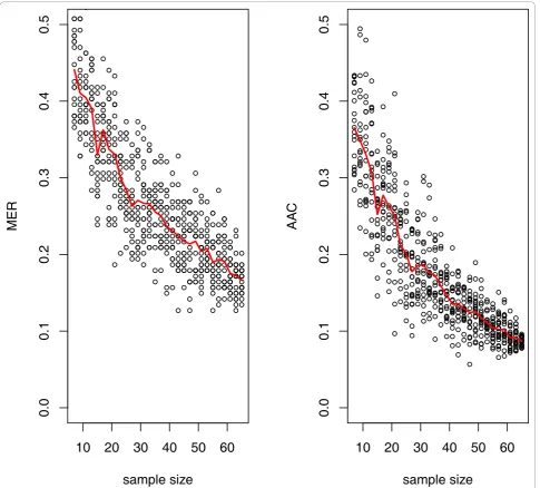
To estimate the effect of training sample size on a clas-sifiers performance we employed learning curves [37]. We used the inverse power-law model

E Y( _train)= + ×Γ  N_train− , Γ, ,  ≥0,

whereE(Ytrain) is the expected value of a performance

metric, e.g. the misclassification error rate MER (MER = 1-ACC, with ACC being the overall model accuracy) or the area above the curve AAC (AAC = 1-AUC), given training sample size Ntrain. Γ is the minimum

classification error that can be expected asNtrain® ∞,

the so called Bayes error which provides the lowest achievable error rate for a given pattern classification problem (Γ=Γ(∞)),gis referred to as the learning rate, andbthe scale. Using SVM classification, the learning curves for AAC and MER are given in Figure 5. SVM was chosen since this approach has been found to give the best or the near best performance for many microarray data sets [38]. For the actual male and female data, the fit resulted in the equations: AAC=0 03 1 39. + . ×N_train−0 716. and MER=0 02 1 052. + . ×N_train−0 597. . From these equa-tions the required sample size can easily be deduced.

20

40

60

80

Sample size

Po

w

er

10

30

50

70

90

110

ID:138036

0

204

06

08

0

Sample size

Po

w

er

10

30

50

70

90

110

ID:19655

Figure 4The resulting power for two markers showing significance after BH adjustments. The power is calculated as the percentage of

times the null hypothesis is rejected. To reach 90% power,Ndiff= 30 samples per group is required for ID:138036 (top), whereas for ID:19655

(bottom)Ndiff= 15 may be enough. From the original 134 samples, 30 cohorts of 2 × 7 subjects each were randomly built. From each cohort,

E.g. for reaching AAC or MER of 10%,Ndisc= 65 andNdisc

= 75, respectively. Hence, MER seems to overestimate the sample sizeNdisc, as this quantity holds only for a given

threshold whereas the AAC gives a global measure for all thresholds. It is important to note that different classifiers will result in different estimates for the AAC and MER and hence another estimate ofNdiscwill be obtained.

In practice it is impossible to reachΓ and only upper bound estimates to it can be reached. The aim is to find the discriminative sample size Ndisc, that guarantees

thatΓ (Ndisc) of the classifier is within some threshold

(e.g = 5%) from the optimal Bayes classifier obtained for infiniteNdisc [39] (that is,Γ(∞) - Γ(Ndisc)≤). Ndisc

may then be obtained by resolving the equation Γ(∞)

-Γ(Ndisc) = . Interestingly, here again the effect size δ

turns out to be the parameter that determines Ndisc. In

the classification context, the effect size measures the distance between the classes. If the pilot study shows a small effect size then it is unlikely that a good discrimi-nator will be easily obtained. The required Ndisc that

maximizes the Γ(Ndisc) implicitly depends on the false

positive rate a [39,40]. Consequently, using those

10 20 30 40 50 60

0.0

0.1

0.2

0.3

0.4

0.5

sample size

AA

C

10 20 30 40 50 60

0.0

0.1

0.2

0.3

0.4

0.5

sample size

MER

Figure 5Learning curve estimation ofNdisc. Cohorts with sample sizes ranging from 2 × 7 - 2 × 65 (given on the x-axis) were arbitrarily

markers that control the FDR should generally produce a good classifier [39,40]. For the 67 male and 67 female profiles, controlling the FDR at 0.05 we are able to define 78 significant peptide markers requiring anNdiff

< 67. With their calculated effect sizes we found that Ndisc = 48 is required to obtain a classifier with 10%

performance short of the optimal Bayes classifier. The analytical method described in [39,40] relies on strong distributional assumptions and seems to be less conser-vative than the learning curve estimation ofNdisc.

Classification

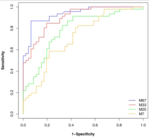
Once a classification rule has been built, its performance must be evaluated. Frequently, complete leave-one-out cross validation (or similar approaches that all are a reflection of the classifier onto the training set) is employed for error estimation. We have investigated if such an approach is indeed appropriate. An SVM-based classifier was built, based on randomly selected 2 × 7, 2 × 20, 2 × 33 datasets, and the entire 2 × 67 cases and controls. As shown in Figure 6 assessment of the

0.0

0.2

0.4

0.6

0.8

1.0

0.0

0.2

0.4

0.6

0.8

1.0

1

−

Specificity

Sensitivity

M67

M33

M20

M7

Figure 6Classification results of an SVM-based classifier. Male and female datasets of size 7, 20, 33, and 67 each were compared. Features

performance based on the complete leave-one-out cross validation (LOOCV) resulted in apparently excellent performance, with the classifier based on 7 cases and controls only appearing to be 100% correct. However, when the classifiers are then tested in the blinded data-set, the results of the classifiers that were built only on a small set of samples could not be verified. As expected, best performance was observed for the classi-fier based on all available data, where the results from the cross validation and the assessment in the indepen-dent dataset are quite similar. These data indicate that results based on the training set only remain question-able, evaluation in an independent set is indeed essential and the ultimate test any procedure must pass. This conclusion supports the findings of [41,42] where the LOOCV error estimate was found to be biased for small samples sizes. For large sample sizes the LOOCV error estimates may be seen as reliable. Therefore we employed the independent test set consisting of 67 male and 67 female samples for evaluation of the perfor-mance of all classifiers. The classification results are reported in Table 3. The results suggest that the perfor-mance of many machine learning algorithms is quite similar and outperforms a simple tree model. Table 3 also suggests that the use of a generalized linear model (GLM) may not be suitable for similar data. GLM, and the tree model seem to be the more sensitive to the variability and the censored structure of the data.

Applications to the CD-DN case study

To further test the applicability of the reported methods we investigated the difference between CD and DN patients using a data set of 120 CD and 120 DN subjects randomly split into 2 60 training and 2 × 60 test data-sets (data available as Additional file 3 and Additional file 4). The differences in this dataset are much more pronounced than the male-female case (Additional file 5). Using the 2 × 60 training data and 10 different ran-dom splits we found that on average 447 peptides may be declared differentially expressed using the adjusted WT. 65% of those markers could be validated in the test data (Additional file 6). The fact that using a pilot study of larger size results in more markers being declared

significant clearly applies here too, as readily seen from the figure in the Additional file 7. The learning curve of this dataset also shows clearly the inverse power law behaviour (Figure in Additional file 8) and suggests that for the CD-DN case fewer subjects than in the male-female comparison may be required to obtain a classifi-cation of comparable performance.

Conclusions

In this report we have examined what requirements have to be met in order to identify significant proteomic biomarkers and establish classifiers that have a high probability of being valid and can be generalized. To avoid misinterpretation: we did not aim at actually iden-tifying biomarkers that we claim to be gender-asso-ciated. The aim of this study was purely to analyse and delineate approaches which ensure a robust study design. In addition, we realize that a study aiming at the identification of biomarkers for classifiers is associated with further challenges, like the above mentioned verifi-cation bias. However, some of the main challenges in biomarker discovery may best be investigated using a well defined experimental system, as the one chosen here. In regard to the first major challenge: how to improve the detection of biomarkers clearly associated to disease, we show that the WT test seems to be best suited for this challenge. However, it also is evident that statistical analysis must be adjusted for multiple testing [43], and we demonstrate the deleterious effects of the avoidance of multiple testing. This effect is even more pronounced when only a small number of samples is being used for the analysis. The un-adjusted p-values obtained from a small sample set are essentially mean-ingless, and are not at all connected with the probability of a certain molecule to be a true biomarker in the test set. In fact, the commonly made silent assumption that among the apparently significant biomarkers (based on unadjusted testing), true significant biomarkers can be found with higher probability than in the apparently non-significant group, could not be verified (data not shown). In our dataset the actual significant features were evenly distributed in these two artificial groups (unadjustedp-values below and above 0.05), which are only generated due to inappropriate statistics, hence they should be considered to be artefacts. This again underlines the notion that unadjusted p-values should not be reported in the absence of other evidence. The lack of statistical power, as well as the unadjusted p-values that erroneously are often considered significant, are mostly a consequence of an incorrect estimation of the true distribution. Due to the relatively high variability observed (in the datasets employed here mostly due to biological variability), the true mean cannot be correctly assessed based on a small set of samples. The incorrect

Table 3 Test errors for different classifiers

Ntrain SVM Hierarchical Bayes

AdaBoost Random Forest

Tree GLM

7 44.7% 32.8% 43.2% 40.2% 48.1% 41.1%

20 40.2% 30.6% 40.2% 35.8% 43.2% 42.5%

33 32.0% 26.1% 23.1% 34.3% 38.1% 38.5%

67 16.4% 21.6% 14.1% 17.1% 26.0% 46.7%

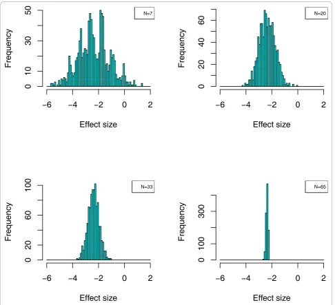
distribution suggests significant differences, which in fact are not true. Only upon investigation of a sufficiently large number of samples can the true mean in the cases and controls be determined. This is also evident from the example shown in Figure 7. We also show that confi-dence in the identified biomarkers can be further improved by resampling of the data, thereby generating a larger number of experiments. Biomarkers that appear significant in each of these experiments, are likely also significant in an independent test set, hence can be

generalized. While such a strategy clearly comes at a cost: the number of biomarkers identified is significantly lower, this strategy may nevertheless represent a pre-ferred option to define likely valid biomarkers, due to the high level of confidence that can be reached. Based on a representative proteomic data set, we also presented methods for answering the second important question: how to estimate the required sample size, both for class comparison (differential sample size) and subject classifi-cation (discriminative sample size). Our data demonstrate

Effect size

Frequency

−

6

−

4

−

2

0

2

0

20

60

100

Effect size

Frequency

−

6

−

4

−

2

0

2

0

100

300

N=65

Effect size

Frequency

−

6

−

4

−

2

0

2

0

103

05

0

N=7

Effect size

Frequency

−

6

−

4

−

2

0

2

02

0

40

60

N=20

Figure 7Effect of sample size on the determination of the distribution of standardized mean-differences. The distribution of a single

peptide, ID:19655, was investigated for four different study designs (N = 7, 20, 33, 67) in 1000 re-sampled distributions out of the complete set of 134 cases and controls each. Typical effect sizeδ= (μmale-μfemale)/s(withμmaleandμfemalebeing the mean logarithmic intensity for a given

that estimation of the differential sample size required for achieving significance in detecting a certain number of specific biomarkers is possible based on resampling from a relatively small dataset. While we have successfully employed only 7 cases and controls, it seems advisable to slightly increase this number to 12 [44]. A similar strat-egy may be adopted for estimating the discriminative sample size required for achieving a predefined confi-dence of a given classifier. Based on the data subse-quently obtained, we used the approach of fitting learning curves. This approach may result in an overesti-mation of the required discriminative sample size. This is in fact beneficial, as it will generally avoid the initiation of an underpowered study. Our data also indicate that testing of biomarkers (e.g. by assessing thep-value) or biomarker models (e.g. by cross validation) in the training set will likely result in an overestimation of their quality. As a consequence, it appears that the quality of biomar-kers or combinations thereof can only be addressed with confidence in an independent test set. Even when analys-ing a significant number of samples, statistics appears to overestimate the value of the potential biomarkers. Statis-tics is based on the assumption of an even distribution of the features across the training and test sets, that the findings can be generalized, and on the association with (in our example) gender only. This is apparently not even the case when using the data from 134 cases and con-trols. The expected result, that 95% of the significant bio-markers should stay significant in the test set, could not be observed. This may indicate that additional variables influence the outcome, and result in an overestimation of the statistical value. Especially when sample sizes are small, even statistically valid results must be interpreted with caution. In such situations, findings should be viewed as tentative and exploratory rather than conclu-sive. Our results further reveal that different machine learning algorithms perform similarly well, and seem to outperform linear classifiers. How-ever, we could also clearly demonstrate that the assessment of the perfor-mance of such a classifier can only be performed on an independent test set, the results obtained from the train-ing set (even when performtrain-ing leave-one-out cross vali-dation) may be misleading. Based on the data presented here, it appears advisable to begin a study aiming at iden-tification of biomarkers or classifiers by performing an analysis of 12 cases and controls, estimate sample size required for certain performance (e.g. accuracy of classifi-cation, level of confidence for biomarkers) based on re-sampling, and then perform the actual study with a suffi-ciently large set of samples. Potential biomarkers must pass WT, adjusted for multiple testing, preferably consis-tently when employing a set of > 30 resamples that each contain e.g. 70% of the available data. Classifiers are best established employing any of the available machine

learning algorithms. The validity of both, biomarkers and classifiers, is generally overestimated in the training set, hence can only be addressed with confidence in an pendent test set. The methods proposed here are inde-pendent on which clinical readout is considered. This fact has been shown by applying them to a dataset com-posed from diabetes type II either with normal kidney function or diabetic nephropathy. This last case study shows that the male-female case is reasonably representa-tive of situations where the search for biomarkers and the classification tasks are rather involved.

Methods

Patients, Procedures and Demographics

Second morning urine samples were collected from apparently healthy volunteers in the course of the medi-cal examination prior to employment at the Hannover Medical School. Consent was given by all participants. Samples were collected in 10 ml Sarstedt urine monov-ettes and frozen immediately after collection without the addition of any preservatives. All samples were col-lected anonymously, only age and gender were recorded. All samples were collected in Germany, and under German law this study does not require IRB approval.

Sample preparation and CE-MS analysis

detail elsewhere [10,17,45]. In short, the detection limit is in the range of 1 fmol, depending on the ionization properties of the individual peptide. This corresponds to 100 -1000 fmol/ml in a crude urine sample (before processing).

Data processing

Mass spectral ion peaks representing identical molecules at different charge states were deconvoluted into single masses using MosaiquesVisu software [47]. Migration time and ion signal intensity (amplitude) were normal-ized based on 29 collagen fragments that serve as inter-nal standards [17]. These interinter-nal polypeptide standards are the result of normal biological processes and have proven to be unaffected by any disease state studied to date (greater than 10,000 samples analysed to date) [48]. The resulting peak list characterizes each peptide by its molecular mass [Da], normalized migration time [min], and normalized signal intensity. All detected peptides were deposited, matched, and annotated in a Microsoft SQL database, allowing further analysis and comparison of multiple samples (patient groups). To establish the identity of peptides observed in different samples, a lin-ear function was employed that allowed, depending on the mass of the polypeptide, a 50 ppm absolute mass deviation for peptides of 800 Da that increased linearly to 100 ppm absolute mass deviation for peptides with a maximum mass of 20 kDa. These values have been found appropriate in several recent studies [11,49,50], as a compromise between avoiding erroneous assignment of the same identity to two different peptides, and assigning two different identities to the same peptide in different analyses, due to mass deviation, especially at low abundance. A similar linear function was used when comparing CE migration times, allowing a 4% absolute deviation. CE-MS data of all individual samples can be accessed in Additional files 1, 2.

Statistical methods, definition of biomarkers and sample classification

All the statistical analyses were implemented with inter-nal scripts, using the R core software [51] as well as the contributed cran-packages ada, Kernlab, Ran-domForest, rpart, WilcoxCv, multtest, and ROCR available at http:// cran.us.r-project.org.

Additional material

Additional file 1: Training set data file for the male-female study. The pivot table CE-MS-male-female-train.xls contains the amplitudes of each peptide in the 67 males (labelled as M...) and 67 females (labelled as F...) used for defining the biomarkers and training the classifiers for differentNtrain. The pivot tables also contain a worksheet named

“Peptides assignment_”that shows the mass (Mass, in Da) and migration time (CE-Time, in min) of peptides assigned to a certain Pep:ID, which is subsequently utilized as the unique identifier in the database.

Additional file 2: Test set data file for the male-female study. The table CE-MS-male-female-test.xls contains the amplitudes in the 67 males and 67 females used for testing the concordance of the biomarkers and estimating the errors of different classifiers. The pivot tables also contain a worksheet named_“Peptides assignment_”that shows the mass (Mass, in Da) and migration time (CE-Time, in min) of peptides assigned to a certain Pep:ID, which is subsequently utilized as the unique identifier in the database.

Additional file 3: Training set data file for the CD-DN study. The pivot table CE-MS-DN-CN-train.xls contains the amplitudes of each peptide in the 60 DN (labelled as DN...) and 60 CD (labelled as CN...) used for defining the biomarkers and training the classifiers for different

Ntrain.

Additional file 4: Test set data file for the CD-DN study. The table CE-MS-DN-CN-test.xls contains the amplitudes in the 60 DN and 60 CD used for testing the concordance of the biomarkers and estimating the errors of different classifiers.

Additional file 5: Typical effect size of a differentially expressed marker in CD versus DN case. The distribution of two peptides, ID:67632 (upper panel) and ID:48751 (lower panel), was investigated in the complete training set (2 × 60) and 1000 re-sampled distributions. Typical effect size_δ= (_μCD-μDN)/s(withμCDandμDNbeing the mean

logarithmic intensity for a given peptide in the CD and DN populations, andsthe pooled standard deviation) is shown. Effect sizes as extreme as -4 and +8 are observed.

Additional file 6: Concordance in the biomarkers using CD-DN data set. The concordance of the markers defined using 60-CD and 60-DN subjects as training set in an independent test set of 60-CD and 60-DN is reported using 10 random splits of the total (2 × 120) data. On average, 447 markers are reported as being significant and 65% of them may be validated on average in the test data.

Additional file 7: Number of significant markers depends on sample size. From the 2 × 60 training data, data sets of sizesNdiffranging from

7 to 60 were built via resampling. At each sample size the number of significant biomarkers (defined as having ap-value after BH adjustments < 0.05) is shown on the vertical axis. The procedure was repeated 10 times to generate the Box-Whisker plots. In all 10 experiments, no biomarkers could be declared significantly differentially expressed below a sample size of 7.

Additional file 8: Learning curve estimation ofNdisc. Cohorts with sample sizes ranging from 2 × 7 - 2 × 58 (given on the x-axis) were arbitrarily generated out of the entire 2 × 60 CD-DN training dataset. 20 repetitions were performed for each size cohort. An SVM-based classifier was built for each dataset and its performance was tested in the independent test set. In the left hand panel the area above the curve AAC (AAC = 1-AUC) for each classifier is shown. The misclassification error rate MER is shown on the right. The red curves represent the mean AAC and mean MER. The inverse power law behaviour is obvious.

List of abbreviationsused

1) AUC: area under the ROC curve; 2) AAC: area above the ROC curve; 3) BH: Benjamini-Hochberg; 4) CE-MS: capillary electrophoresis coupled mass spectrometry; 5) CD: diabetes type II with normal kidney function; 6) DN: diabetic nephropathy; 7) ESI: electro-spray ionization; 8) FDR: false discovery rate; 9) GLM: generalized linear model; 10) LC-MS: liquid chromatography coupled mass spectrometry; 11) LOD: limit of detection; 12) LOOCV: leave-one-out cross validation; 13) MALDI: matrix assisted laser desorption ionization; 14) MER: misclassification error rate; 15)Ndiff: differential sample

size; 16)Ndisc: discriminative sample size; 17) ROC: receiver operating

characteristic; 18) SQL: structured query language; 19) SVM: support vector machine; 20) WT: Wilcoxon rank sum test.

Acknowledgements

FP7 DECanBio (201333) and by the European Community’s 7th Framework Programme, grant agreement HEALTH-F2-2009-241544 (SysKID). JPS acknowledges financial support from the Agence Nationale pour la Rechérche (ANR-07-PHYSIO-004-01), and support by Inserm, the_“Direction Régional Clinique”(CHU de Toulouse, France) under the Interface program. WK is supported by the Science Foundation Ireland under Grant No. 06/CE/ B1129.

Author details

1_{Mosaiques diagnostics and therapeutics, Hannover, Germany.}2_{Water and}

Environment Research Group, School of Engineering, University of Glasgow, Glasgow, UK.3_{Computer Science Department, University of Geneva, Geneva,}

Switzerland.4_{Laboratory of Tropical Crop Improvement, Katholieke}

Universiteit, Leuven, Belgium.5The Beatson Institute for Cancer Research and Sir Henry Wellcome Functional Genomics Facility, University of Glasgow, Glasgow, UK.6Systems Biology Ireland, Conway Institute, Belfield, Dublin 4, Ireland.7_{Institut National de la Santé et de la Recherche Médicale (INSERM),}

U858, Toulouse, France.8Université Toulouse III Paul-Sabatier, Institut de Médecine Moleculaire de Rangueil, Equipe n° 5, IFR150, Toulouse, France.

9_{Department of Nephrology, Hannover Medical School, Hannover, Germany.} 10_{BHF Glasgow Cardiovascular Research Centre, University of Glasgow,}

Glasgow, UK.11_{Research Foundation, Academy of Athens, Athens, Greece.} 12

Department of Statistical Science, University College London, London, UK.

Authors’contributions

All authors participated in the design of the study. MD and HM performed the statistical analysis. HM performed the CE-MS analysis and initial data evaluation. AK, KH, SC, MD, and MG developed the high dimensional models. JPS and MH were involved in the recruitment of study participants. All authors were involved in drafting the manuscript, have read and approved the final manuscript.

Authors_’information

Joost P Schanstra, Antonia Vlahou and Harald Mischak are all members of EUROKUP

Received: 3 November 2010 Accepted: 10 December 2010 Published: 10 December 2010

References

1. Rifai N, Gillette MA, Carr SA:Protein biomarker discovery and validation: the long and uncertain path to clinical utility.Nat Biotechnol2006,

24(8):971-83, [Rifai1, Nader Gillette, Michael A Carr, Steven A Research Support, N.I.H., Extramural Research Support, Non-U.S. Gov’t Review United States Nature biotechnology Nat Biotechnol. 2006 Aug;24(8):971-83.]. 2. Listgarten J, Emili A:Practical proteomic biomarker discovery: taking a

step back to leap forward.Drug Discov Today2005,10(23-24):1697-702. 3. Petricoin EF, Ardekani AM, Hitt BA, Levine PJ, Fusaro VA, Steinberg SM,

Mills GB, Simone C, Fishman DA, Kohn EC, Liotta LA:Use of proteomic patterns in serum to identify ovarian cancer.Lancet2002,

359(9306):572-7.

4. McLerran D, Grizzle WE, Feng Z, Thompson IM, Bigbee WL, Cazares LH, Chan DW, Dahlgren J, Diaz J, Kagan J, Lin DW, Malik G, Oelschlager D, Partin A, Randolph TW, Sokoll L, Srivastava S, Thornquist M, Troyer D, Wright GL, Zhang Z, Zhu L, Semmes OJ:SELDI-TOF MS whole serum proteomic profiling with IMAC surface does not reliably detect prostate cancer.Clin Chem2008,54:53-60.

5. Diamandis EP:Point: Proteomic patterns in biological fluids: do they represent the future of cancer diagnostics?Clin Chem2003,49(8):1272-5. 6. Ransohoff DF:Bias as a threat to the validity of cancer molecular-marker

research.Nat Rev Cancer2005,5(2):142-9.

7. Mischak H, Apweiler R, Banks RE, Conaway M, Coon J, Dominiczak A, Ehrich JHH, Fliser D, Girolami M, Hermjakob H, Hochstrasser D, Jankowski J, Julian BA, Kolch W, Massy ZA, Neusuess C, Novak J, Peter K, Rossing K, Schanstra J, Semmes OJ, Theodorescu D, Thongboonkerd V, Weissinger EM, Van Eyk JE, Yamamoto T:Clinical proteomics: A need to define the field and to begin to set adequate standards.PROTEOMICS - Clinical Applications2007,1(2):148-156[http://dx.doi.org/10.1002/prca.200600771]. 8. Decramer S, Gonzalez de Peredo A, Breuil B, Mischak H, Monsarrat B,

Bascands JL, Schanstra JP:Urine in clinical proteomics.Mol Cell Proteomics

2008,7(10):1850-62.

9. Fliser D, Novak J, Thongboonkerd V, Argiles A, Jankowski V, Girolami MA, Jankowski J, Mischak H:Advances in Urinary Proteome Analysis and Biomarker Discovery.J Am Soc Nephrol2007,18(4):1057-1071[http://jasn. asnjournals.org/cgi/content/abstract/18/4/1057].

10. Haubitz M, Good DM, Woywodt A, Haller H, Rupprecht H, Theodorescu D, Dakna M, Coon JJ, Mischak H:Identification and validation of urinary biomarkers for differential diagnosis and evaluation of therapeutic intervention in anti-neutrophil cytoplasmic antibody-associated vasculitis.Mol Cell Proteomics2009,8(10):2296-307.

11. Good DM, Zürbig P, Argilés n, Bauer HW, Behrens G, Coon JJ, Dakna M, Decramer S, Delles C, Dominiczak AF, Ehrich JHH, Eitner F, Fliser D, Fromm-berger M, Ganser A, Girolami MA, Golovko I, Gwinner W, Haubitz M, Herget-Rosenthal S, Jankowski J, Jahn H, Jerums G, Julian BA, Kellmann M, Kliem V, Kolch W, Krolewski AS, Luppi M, Massy Z, Melter M, Neusüss C, Novak J, Peter K, Rossing K, Rupprecht H, Schanstra JP, Schiffer E, Stolzenburg JU, Tarnow L, Theodorescu D, Thongboonkerd V, Vanholder R, Weissinger EM, Mischak H, Schmitt-Kopplin P:Naturally Occurring Human Urinary Peptides for Use in Diagnosis of Chronic Kidney Disease.Molecular and Cellular Proteomics2010,9(11):2424-2437[http://www.mcponline.org/ content/9/11/2424.abstract].

12. Mischak H, Allmaier G, Apweiler R, Attwood T, Baumann M, Benigni A, Bennett SE, Bischo R, Bongcam-Rudloff E, Capasso G, Coon JJ, DHaese P, Dominiczak AF, Dakna M, Dihazi H, Ehrich JH, Fernandez-Llama P, Fliser D, Frokiaer J, Garin J, Girolami M, Hancock WS, Haubitz M, Hochstrasser D, Holman RR, Ioannidis JPA, Jankowski J, Julian BA, Klein JB, Kolch W, Luider T, Massy Z, Mattes WB, Molina F, Monsarrat B, Novak J, Peter K, Rossing P, Sanchez-Carbayo M, Schanstra JP, Semmes OJ, Spasovski G, Theodorescu D, Thongboonkerd V, Vanholder R, Veenstra TD, Weissinger E, Yamamoto T, Vlahou A:Recommendations for Biomarker Identification and Qualification in Clinical Proteomics.Science Translational Medicine2010,2(46):46ps42[http://stm.sciencemag.org/ content/2/46/46ps42.abstract].

13. Alonzo TA, Kittelson JM:A novel design for estimating relative accuracy of screening tests when complete disease verification is not feasible. Biometrics2006,62(2):605-12, [Alonzo, Todd A Kittelson, John M R01 GM54438/GM/NIGMS NIH HHS/United States Comparative Study Research Support, N.I.H., Extramural Research Support, Non-U.S. Gov’t United States Bio-metrics Biometrics. 2006 Jun;62(2):605-12.].

14. Buzoianu M, Kadane JB:Adjusting for verification bias in diagnostic test evaluation: a Bayesian approach.Stat Med2008,27:2453-2473.

15. Page JH, Rotnitzky A:Estimation of the disease-specific diagnostic marker distribution under verification bias.Computational Statistics and Data Analysis2009,53(3):707-717[http://www.sciencedirect.com/science/article/ B6V8V-4SX9FTT-1/2/a708b210a358c83a359bd1c2ca7bef7f].

16. Mischak H, Coon JJ, Novak J, Weissinger EM, Schanstra JP, Dominiczak AF:

Capillary electrophoresis-mass spectrometry as a powerful tool in biomarker discovery and clinical diagnosis: an update of recent developments.Mass Spectrom Rev2009,28(5):703-24.

17. Jantos-Siwy J, Schiffer E, Brand K, Schumann G, Rossing K, Delles C, Mischak H, Metzger J:Quantitative urinary proteome analysis for biomarker evaluation in chronic kidney disease.J Proteome Res2009,

8:268-81.

18. Wang P, Tang H, Zhang H, Whiteaker J, Paulovich AG, Mcintosh M:

Normalization regarding non-random missing values in high-throughput mass spectrometry data.Pac Symp Biocomput2006, 315-326.

19. Helsel R:Nondetects and data analysis: statistics for censored environmental data.New York: Wiley-Interscience; 2005.

20. Taylor S, Pollard K:Hypothesis tests for point-mass mixture data with application to‘omics data with many zero values.Stat Appl Genet Mol Biol2009,8:Article 8.

21. Broadhurst D, Kell D:Statistical strategies for avoiding false discoveries in metabolomics and related experiments.Metabolomics2006,2(4):171-196 [http://dx.doi.org/10.1007/s11306-006-0037-z].

22. Dakna M, He Z, Yu WC, Mischak H, Kolch W:Technical, bioinformatical and statistical aspects of liquid chromatography-mass spectrometry (LC-MS) and capillary electrophoresis-mass spectrometry (CE-MS) based clinical proteomics: a critical assessment.J Chromatogr B Analyt Technol Biomed Life Sci2009,877:1250-1258.

23. Oberg AL, Vitek O:Statistical Design of Quantitative Mass Spectrometry-Based Proteomic Experiments.Journal of Proteome Research2009,

24. Benjamini Y, Hochberg Y:Controlling the False Discovery Rate: A Practical and Powerful Approach to Multiple Testing.Journal of the Royal Statistical Society. Series B (Methodological)1995,57:289-300[http://vorlon.case.edu/ ~sray/mlrg/controlling_fdr_benjamini95.pdf].

25. Hemelrijk J:Note on Wilcoxon’s Two-Sample Test when Ties are Present. Annals of Mathematical Statistics1952,23:133-135.

26. Soares AJ, Santos M, Trugilho M, Neves-Ferreira A, Perales J, Domont G:

Differential proteomics of the plasma of individuals with sepsis caused by Acinetobacter baumannii.Journal of Proteomics2009,73(2):267-278 [http://www.sciencedirect.com/science/article/B8JDC-4X9NVD1-1/2/ e97759e56b52f471a9361b9d05d3072b].

27. Matsubara J, Ono M, Honda K, Negishi A, Ueno H, Okusaka T, Furuse J, Furuta K, Sugiyama E, Saito Y, Kaniwa N, Sawada J, Shoji A, Sakuma T, Chiba T, Saijo N, Hirohashi S, Yamada T:Survival Prediction for Pancreatic Cancer Patients Receiving Gemcitabine Treatment.Molecular and Cellular Proteomics2010,9(4):695-704[http://www.mcponline.org/content/9/4/695. abstract].

28. Ma Y, Peng J, Huang L, Liu W, Zhang P, Qin H:Searching for serum tumor markers for colorectal cancer using a 2-D DIGE approach.Electrophoresis

2009,30(15):2591-2599.

29. Altman DMD, TN B, MJ G:Statistics with Confidence: Confidence intervals and statistical guidelines.London: BMJ Books;, 2 2000.

30. Cairns DA, Barrett JH, Billingham LJ, Stanley AJ, Xi-narianos G, Field JK, Johnson PJ, Selby PJ, Banks RE:Sample size determination in clinical proteomic profiling experiments using mass spectrometry for class comparison.Proteomics2009,9:74-86.

31. Jackson D, Herath A, Swinton J, Bramwell D, Chopra R, Hughes A, Cheeseman K, Tonge R:Considerations for powering a clinical proteomics study: Normal variability in the human plasma proteome.PROTEOMICS -CLINICAL APPLICATIONS2009,3(3):394-407.

32. Efron B, Tibshirani R:An Introduction to the Bootstrap.Boca Raton: Chapman & Hall/CRC; 1993.

33. Strimmer K:A unified approach to false discovery rate estimation.BMC Bioinformatics2008,9:303.

34. Lesaffre E, Scheys I, Frohlich J, Bluhmki E:Calculation of power and sample size with bounded outcome scores.Stat Med1993,12:1063-1078. 35. Walters SJ:Sample size and power estimation for studies with health

related quality of life out-comes: a comparison of four methods using the SF-36.Health Qual Life Outcomes2004,2:26.

36. Lin WJ, Hsueh HM, Chen JJ:Power and sample size estimation in microarray studies.BMC Bioinformatics2010,11:48.

37. Mukherjee S, Tamayo P, Rogers S, Rifkin R, Engle A, Campbell C, Golub TR, Mesirov JP:Estimating dataset size requirements for classifying DNA microarray data.J Comput Biol2003,10(2):119-42.

38. Kenneth RH, Caimiao W:Learning Curves in Classification With Microarray Data.Seminars in oncology2010,37:65-68.

39. Dobbin KK, Zhao Y, Simon RM:How large a training set is needed to develop a classifier for microarray data?Clin Cancer Res2008,14:108-14. 40. Dobbin KK, Simon RM:Sample size planning for developing classifiers

using high-dimensional DNA microarray data.Biostatistics2007,8:101-117. 41. Braga-Neto UM, Dougherty ER:Is cross-validation valid for small-sample

microarray classification?Bioinformatics2004,20(3):374-80. 42. Molinaro AM, Simon R, Pfeiffer RM:Prediction error estimation: a

comparison of resampling methods.Bioinformatics2005,21(15):3301-7. 43. Dudoit S, van der Laan M:Multiple Testing Procedures with Applications

to Genomics.New York: Springer; 2008.

44. Hogg R, Tannis E:Probability and Statistical Inference.Prentice Hall: Pearson;, 8 2010.

45. Theodorescu D, Wittke S, Ross MM, Walden M, Conaway M, Just I, Mischak H, Frierson HF:Discovery and validation of new protein biomarkers for urothelial cancer: a prospective analysis.Lancet Oncol

2006,7(3):230-40.

46. Wittke S, Mischak H, Walden M, Kolch W, Radler T, Wiedemann K:Discovery of biomarkers in human urine and cerebrospinal fluid by capillary electrophoresis coupled to mass spectrometry: towards new diagnostic and therapeutic approaches.Electrophoresis2005,26(7-8):1476-87. 47. Neuhoff N, Kaiser T, Wittke S, Krebs R, Pitt A, Bur-chard A, Sundmacher A,

Schlegelberger B, Kolch W, Mischak H:Mass spectrometry for the detection of differentially expressed proteins: a comparison of surface-enhanced laser desorption/ionization and capillary electrophoresis/mass spectrometry.Rapid Commun Mass Spectrom2004,18(2):149-56.

48. Coon JJ, Zurbig P, Dakna M, Dominiczak AF, Decramer S, Fliser D, Frommberger M, Golovko I, Good DM, Herget-Rosenthal S, Jankowski J, Julian BA, Kellmann M, Kolch W, Massy Z, Novak J, Rossing K, Schanstra JP, Schiffer E, Theodorescu D, Vanholder R, Weissinger EM, Mischak H, Schmitt-Kopplin P:CE-MS analysis of the human urinary proteome for biomarker discovery and disease diagnostics.Proteomics Clin Appl2008,2:964. 49. Alkhalaf A, Zürbig P, Bakker SJL, Bilo HJG, Cerna M, Fischer C, Fuchs S,

Janssen B, Medek K, Mischak H, Roob JM, Rossing K, Rossing P, Rychlík I, Sourij H, Tiran B, Winklhofer-Roob BM, Navis GJ, for the PREDICTIONS Group:Multicentric Validation of Proteomic Biomarkers in Urine Specific for Diabetic Nephropathy.PLoS ONE2010,5(10):e13421[http://dx.doi.org/ 10.1371%2Fjournal.pone.0013421].

50. Maahs DM, Siwy J, Argilés n, Cerna M, Delles C, Dominiczak AF, Gayrard N, Iphöfer A, Jänsch L, Jerums G, Medek K, Mischak H, Navis GJ, Roob JM, Rossing K, Rossing P, Rychlík I, Schiffer E, Schmieder RE, Wascher TC, Winklhofer-Roob BM, Zimmerli LU, Zürbig P, Snell-Bergeon JK:Urinary Collagen Fragments Are Significantly Altered in Diabetes: A Link to Pathophysiology.PLoS ONE2010,5(9):e13051[http://dx.doi.org/10.1371% 2Fjournal.pone.0013051].

51. R Development Core Team:R: A Language and Environment for Statistical Computing.R Foundation for Statistical Computing, Vienna, Austria; 2010 [http://www.R-project.org], [ISBN 3-900051-07-0].

doi:10.1186/1471-2105-11-594

Cite this article as:Daknaet al.:Addressing the Challenge of Defining

Valid Proteomic Biomarkers and Classifiers.BMC Bioinformatics2010

11:594.

Submit your next manuscript to BioMed Central and take full advantage of:

• Convenient online submission

• Thorough peer review

• No space constraints or color figure charges

• Immediate publication on acceptance

• Inclusion in PubMed, CAS, Scopus and Google Scholar

• Research which is freely available for redistribution