promoting access to White Rose research papers
Universities of Leeds, Sheffield and York
http://eprints.whiterose.ac.uk/
This is an author produced version of a paper published in Annals of Operations Research.
White Rose Research Online URL for this paper:
Published paper
Adcock, C.J. (2010) Asset pricing and portfolio selection based on the multivariate extended skew-Student-t distribution, Annals of Operations Research, 176 (1), pp. 221-234
Asset Pricing and Portfolio Selection Based on the Multivariate Extended Skew-Student-t Distribution
by
C J Adcock
The University of Sheffield, UK
Abstract
The returns on most financial assets exhibit kurtosis and many also have probability distributions that possess skewness as well. In this paper a general multivariate model for the probability distribution of assets returns, which incorporates both kurtosis and skewness, is described. It is based on the multivariate extended skew-Student-t distribution. Salient features of the distribution are described and these are applied to the task of asset pricing. The paper shows that the market model is non-linear in general and that the sensitivity of asset returns to return on the market portfolio is not the same as the conventional beta, although this measure does arise in special cases. It is shown that the variance of asset returns is time varying and depends on the squared deviation of market portfolio return from its location parameter. The first order conditions for portfolio selection are described. Expected utility maximisers will select portfolios from an efficient surface, which is an analogue of the familiar mean-variance frontier, and which may be implemented using quadratic programming.
Key words: Capital Asset Pricing Model, Efficient frontier, Market Model, Multivariate skew-normal distribution, Multivariate Student distribution, Portfolio selection, Utility functions
Correspondence Address
C J Adcock
The Management School University of Sheffield 9, Mappin Street Sheffield, S1 4DT UK
Tel: +44 (0)114 222 3402 Fax: +44 (0)114 222 3348 Email: [email protected]
1. Introduction
Modern portfolio theory makes extensive use, both explicit and implicit, of the normal distribution. Two aspects of the importance of normality of asset returns are as follows. First, when asset returns follow a multivariate normal distribution, the market model, the equation that links assets returns to returns on the market portfolio, is linear and may be correctly estimated using OLS. Secondly, investors who select portfolios by maximising the expected utility of return will always be located on Markowitz’ mean-variance efficient frontier. This well-known feature is a consequence of Stein’s lemma, Stein (1981). In reality, it is accepted that asset returns are not normally distributed. It is now common practice to recognise the non-normality inherent in returns and to build more appropriate models. Nowadays, there is a very wide variety of models, ARCH/GARCH and neural networks to name just two, that is in common use. For applications which require models of the multivariate distribution of asset returns, there has been substantial growth in recent years of the use of copulae in finance; see for example the recent book by Cherubini et al (2004). Such models, however, can leave two issues unresolved. These are (a) the correct form of the market model and (b) the choice of an appropriate utility function for portfolio selection.
The form of the market model is an important issue for the following reason. It is conventionally assumed that this takes the familiar linear regression form. However, the OLS model makes strong assumptions about the form of the multivariate probability distribution of asset returns. In the absence of normality, OLS is not the optimal estimation method. Furthermore in the absence of elliptical symmetry there is no guarantee that the relationship between asset returns and market returns is linear. The choice of utility function is also an important consideration. Under some return distributions, certain choices of the functional form of the utility function are prohibited because the expected values do not exist. From a more pragmatic perspective, the question of whether there is a utility function that is “optimal” in some sense for a given return distribution is always likely to receive attention. In addition, to date anyway, the use of copulae is restricted to a small number of dimensions. This does not of course limit their importance or usefulness, but does mean that applications like large-scale portfolio selection require simplifying assumptions to be made.
The past two decades has seen the development of a large body of theory concerning multivariate probability distributions which are elliptically symmetric. The standard source reference is the well-known monograph by Fang et al (1990). These distributions result in market models which are linear, although of course OLS is not the optimal method for parameter estimation. Papers by Liu (1994), Landsman (2006) and Landsman and Nešlehová (2008) present extensions to Stein’s lemma which indicate that, ceteris paribus, there is a single efficient frontier for all expected utility maximisers.
is readily apparent that the use of a single multivariate distribution requires that compromises be made in the ability to estimate marginal distributions. The view taken in this work is that the gains offered by a coherent multivariate model offset the effects of such compromises. Furthermore, as is very well known, estimation error for associated with models used in finance is almost always substantial and it is debatable whether a more complex model will yield superior properties in practice.
The MEST distribution described in this paper is a development of the multivariate skew-normal (MSN) distribution introduced by Azzalini and Dalla-Valle (1996), henceforth AZ&DV. The MSN distribution was first used as a model for returns in finance in Adcock and Shutes (2001), henceforth A&S, who introduced an extension of the model which is often referred to the multivariate extended skew-normal or MESN distribution.
The motivation for an extended skew-Student-t model as distinct to the skew-normal is that kurtosis is almost always present in asset returns. The ability to incorporate fat-tails as well as skewness is therefore an important practical consideration. The use of a Student model is motivated to some extent by tractability, but also by a number of papers spanning several decades that indicate that the Student distribution is a useful model for fat-tailed returns. Two examples of such work include the well-known papers by Praetz (1972) and Blattberg and Gonedes (1974) and the study of returns on European securities by Aparicio and Estrada (2001).
Development of the multivariate skew-Student-t and related distributions is an active area of research. The publication of initial papers by Branco and Dey (2001), Azzalini and Capitanio (2003) and Sahu et al (2003) has been followed by articles by several authors including Arellano-Valle and Genton (2005), Arrellano-Valle et al (2006), Arrellano-Valle and Azzalini (2006) and Azzalini and Genton (2008). An extended skew Student distribution and many of its properties are described in Arellano-Valle and Genton (2008), henceforth AV&G.
There are also several papers which present other multivariate distributions, all of which possess skewness and which are based on the Student distribution. Examples of such work are in Jones (2001, 2002), Jones and Faddy (2003) and Bauwens and Laurent (2005). There is also a univariate skewed t distribution, which was introduced by McDonald and Xu (1995). This has been generalised and applied to financial data in Theodossiou (1998), who calls the model the skewed generalized t distribution. However, no multivariate form of this model appears in the literature.
investors’ utility function. Under the MEST distribution, portfolio selection may be implemented using quadratic programming.
The structure of the paper is as follows. Section 2 contains a short summary of the multivariate extended skew-normal distribution. Section 3 describes the derivation and probability density function of the MEST distribution that is used in this paper and presents properties that are required in subsequent sections. This includes the general conditional distribution for the case when the vector of returns R is partitioned into two components R1 and R2 say and R1 is taken as given. In section 4 this is applied to the situation where R1 is the scalar return on a market portfolio. The resulting market model is shown to be non-linear in general. Section 5 is concerned with portfolio selection and efficient set mathematics. Section 6 concludes the paper. There are two short appendices.
In the text of this paper, the word beta refers to the conventional measure of risk; that is the covariance of asset returns with the return on the market portfolio divided by market variance. The notation β is reserved for a different definition of risk that arises with market models based on the MEST distribution. However, as is shown in the paper, there are cases where β is essentially the same as beta. Notation is that in common use.
2. The Multivariate Extended Skew-Normal Distribution
There are several ways of deriving multivariate skew-normal distributions. With financial applications in mind, the following method from A&S is used. Let Ybe an n-vector with the full rank multivariate normal distribution N
(
µ,Σ)
. Let X be a scalar random variable which is independent of Y and which has a normal distribution with mean τ, variance 1 and is left truncated at zero. The vector of variables R =Y+λX has a multivariate extended skew-normal, henceforth MESN, distribution. This may be interpreted as follows. If R denotes returns on risky financial assets over a single period, the definition above means that each return Ri has two components: Yiwhich is normally distributed with mean µi and a skewness shock λiX . The shock is generated by the single variable X . The sensitivity of security i to the shock is λi, which may take any real value including zero. The skewness shock may be interpreted as a departure from market efficiency in the sense of Fama (1970).Using the notation above, the distribution of the vector of returns R has probability density function
( )
(
)
( )λ λ
λ
) µ (
λλ
,
λ
µ
; τ Φ τ τ
n φ
f Φ
− +
− −
+ +
+ =
1 T 1
1 T T
Σ Σ
r
Σ
r
r , (1.)
( )
τΦ denotes the standard normal distribution function evaluated at τ. When τ takes the value zero, this is equivalent to the corresponding result in AZ&DV with a change of notation. The explicit use of non-zero values of τ facilitates some subsequent manipulations of the density. It also creates a richer family of probability distributions. The distribution at (1.) is denoted R~ MESN
(
µ,Σ,λ,τ)
. Moments and related properties of this distribution, expressed in the above notation, are described in A&S. AZ&DV show that when the vector R is partitioned into two components,1
R and R2, containing n1 and n2 =n−n1elements respectively, the conditional distribution of R2 given that R1 =r1 is multivariate skew-normal of the same family. In the usual way, partition as µ, Σand λ as
= = = 2 1 22 21 12 11 2
1 , ,
λ λ λ µ µ µ Σ Σ Σ Σ V .
The conditional distribution of R2 given that R1 =r1 is MESN
(
µ2|1,Σ2|1λ2|1,τ2|1)
where . λ λ ) µ ( λ , λ λ λ λ λ , ), µ ( µ µ | | | | 1 1 11 T 1 1 1 1 11 T 1 1 2 1 1 11 T 1 1 1 11 21 2 1 2 12 1 11 21 22 1 2 1 1 1 11 21 2 1 2 1 1 − − − − − − + − + τ = + − = − = − + = Σ r Σ Σ Σ Σ Σ Σ Σ Σ Σ r Σ Σ τ
A&S apply this to the situation where R2 represents individual asset returns and R1, which is a scalar variable, is the return on the market portfolio, Rp say. It will be apparent from the form of the parameters in the above equations that the market model, the expected value of the vector of asset returns conditional on the return on the market portfolio, is non-linear in rp, the given value of the market return. This model may also be applied to general regression. In this case, the conditioning vector
1
R represents selected explanatory variables. The vector R1 may have a multivariate normal distribution, in which case λ1 =0. In this case, the regression model that links the dependent variables R2 to the independent variables r1 is linear in r1.
3. The Multivariate Extended Skew-Student-t Distribution
The MEST distribution may be derived using the standard form of multivariate Student distribution (see for example Johnson & Kotz, 1972, page 162 et sec or Bernardo and Smith, 1994, page 435 and 441). The vector R is defined as above, except that the vector
− − τ X µ Y ,
now has a centred multivariate Student distribution with υ degrees of freedom and dispersion matrix equal to
1 T 0 0 Σ ,
with the variable X being left-truncated at zero. The joint distribution of Y and X has probability density function proportional to
[
1 {( ) ( ) ( ) }/]
2( 1) ( )1 2
1 − + −τ τ
−
+ − − + +
υ
n
υ
T µ x υ T
µ Σ y
y ,
for x>0 where Tυ
( )
τ denotes the distribution function for the Student-t distribution with υ degrees of freedom evaluated at τ. Standard transformation of the variables gives the joint distribution of R and X . Writing this joint probability density in the conditional form f( ) ( )
x|r f r and integrating with respect to x gives the MEST distribution, with probability density function
( )
(
)
{
}
) ( υ T T υ τ Q T τ υ n υ n υ T υ T τ n t f τ + − + − − + + + + + = λ λ λ µ λ µ λλ λ µ r 1 1 ) , , , , ( 1 1 ) ( , , ; Σ Σ r Σ r Σr . (2.)
The quadratic form Q(r,µ,λ,τ,Σ)is defined as
Q τ
(
τ)
T(
T)
(
τ)
λ µ λλ λ µ λµ Σ = r− − Σ+ − r− −
r, , , , ) 1
( . (3.)
The function
(
υ)
nThe distribution derived in Sahu et al (2003) uses more than one skewness variable. An extended MEST distribution with more that one truncated variable is also reported in AV&G and Adcock (2008). It is a development of similar extensions to the multivariate skew normal distribution described in Gonzàlez-Farías et al (2004) and Arellano-Valle and Azzalini (2006). As AV&G rightly remark these “are … generalizations that are of interest from a theoretical point of view”. As the papers by Horrace (2005) and Adcock (2007) make clear, the computational difficulties alone are substantial.
The rest of this section presents properties of the MEST distribution, which are used in Section 4. A number of other properties of the distribution which are not required are omitted.
3.1 Linear Transformations of Multivariate Extended Skew-Student-t Variables
When R~MEST
(
µ,Σ,λ,τ,υ)
, the linear transformation ΜR+η, where Μis an
m× matrix of rank less that or equal to n is distributed as
(
Μµ η,ΜΣΜT,Μλ,τ,υ)
MEST + . The proof of this is omitted. Allowing for changes in notation, this result is essentially the same as proposition 5 of AV&G.
3.2 A New Elliptically Symmetric Distribution
When the λ equals the zero vector, the probability density function is
( )
(
)
{
}
) ( υ T
υ τ Q
τ υ
n υ n υ T υ n
t r f
τ
+ + +
= r;µ,Σ, 1 (r,µ,0, ,Σ) .
The effect of τ >0
( )
<0 is to increase (decrease) the peakedness of the density around 0R= when compared with the standard multivariate Student density. This distribution is also reported in AV&G, who note that certain values of τ will produce lighter tails than the normal distribution. From the perspective of finance, the potential interest in this distribution lies in the fact that it can be more peaked than the Student distribution. It may therefore have the ability to describe the returns on assets which are thinly traded and for which the frequency of zero returns is higher than that predicted by Student’s t. The following result is an interesting by-product of this distribution.
Lemma 1
Let Ybe an n-vector which has a multivariate Student distribution with location parameter vector µ, scale matrix Σ and υ degrees of freedom. Let the quadratic form Q(y,µ,λ,τ,Σ) be as defined at equation (3.). The following result holds
) ( υ T υ ) ,0, , , Q( 1
τ υ
n υ n υ T
E = τ
+ +
+
Σ
0 µ
3.3 Expectation and Variance Covariance Matrix of R
Direct evaluation of the higher unconditional moments of the distribution of R, when they exist, is not straightforward and is beyond the scope of this paper. However, it is straightforward to show that for υ>1 and υ>2, respectively
( )
{
(
)
}
{
(
)
}
( )
(
)
{
}
( )
{
(
(
)
)
}
{
(
) ( )
}
( )
,) (
2 τξ τ υT τ υ 2 /υ υ 2T τ η τ X
E
, τ ξ τ ) ( T 1 υ υ τ 1 τ υt τ X E
υ υ
2
υ υ
υ υ
2
υ
= −
− +
− = −
+ = τ − +
+ =
− τ
where )tυ(τ denotes the density function for the Student-t distribution with υ degrees of freedom evaluated at τ. The unconditional expected value of R is
( )
τ ξ (τ)E R = µ+λ +λ υ . The conditional covariance matrix of R given X =x is
(
|x)
υ{1(
x τ)
2/υ}( )
υ-1ar
v R = + − Σ . For υ>2, the unconditional covariance matrix of R is
( )
{
( )
} ( )
{
( )
( )
}
Tυ υ
υ τ υ υ- η τ ξ τ
η υ
ar
v R = 1+ Σ 1 + − 2 λλ .
When all elements of λ are equal to zero, the covariance matrix is a function of τ, even though this variable does not then affect expected returns. Since the above result holds for all values of Σ and λ the following
{
1+η (τ) υ}
≥0,{
η (τ)−ξ (τ)2}
≥0υ υ
υ ,
hold for all values of τ. As υ→∞, the covariance matrix of Rtends to the corresponding expression for the MESN distribution in Section 2.
3.4 Conditional Distributions
Let R be partitioned into two components, R1 and R2, containing n1 and
1 2 n n
n = − elements respectively and the parameters µ, Σ, λ partitioned correspondingly. The conditional distribution of R2 given that R1 =r1is also MEST. The derivation is omitted, but the method is the same as that briefly described in Section 2 or in AZ&DV. The conditional distribution of R2 given R1 =r1 is
(
µ2|1, 2|1,λ2|1,τ2|1,υ+n1)
(
)
(
) (
)
(
1)
(
1)
,) ( ) ( , 1 1 , ) 1 ( ), ( 1 1 11 1 1 1 1 1 11 1 1 | 2 1 1 1 11 1 1 1 11 21 2 1 | 2 12 1 11 21 22 1 1 | 2 1 1 1 11 21 2 1 | 2 λ λ µ λ λ λ λ λ λ µ µ µ − − − − − − + + − + τ + = τ + + + − = − + + = − + = Σ r Σ Σ Σ Σ Σ Σ Σ Σ Σ r Σ Σ T T 1 1 T 1 υ Q υ n υ n υ υ Q υ υ Q ) n (υ υ
with Q1 =Q(r1,µ1,λ1,τ,Σ11). The expected value of R2 given that R1 =r1is a non-linear function r1. The details of three cases of the conditional distribution: (i)
0
=
1
λ ; (ii) at least one element of λ1is non-zero and (iii) λ2|1 =0 are described in Appendix A. The vector λ2|1is referred to as conditional skewness.
4. The Market Model
When R represents the returns on a set of assets, the return on the market portfolio or market proxy is given by the linear transformation TR
p
R =w , where the vector w represents the weights of each asset. The market model, in which R1 is the now scalar variable Rp may be established using the results above. From the definition of the distribution, it follows that Rphas a (univariate) extended skew-Student-t distribution
(
τ,υ)
EST
R T T T
p ~ w µ,w Σw,w λ, , equivalently
(
µ ,σ ,λp,τ,υ)
2p p
EST . The distribution of a vector of asset returns R2 given that Rp =rp follows the MEST distribution with
1
υ+ degrees of freedom and parameters
(
)
(
)
(
)
(
)
(
/)
. , / 2 , 1 ) 1 ( , 22 2 − + + = − + = + + − + + = + + + − = 2 p σ 2 p 2 p 2 p 2 p c σ σ υ / λ 1 υ c 1 2 p /σ p )λ p µ p (r τ υ 1) (υ c τ 1 υ υ) c υ(1 / λ 1 p λ c T c p p c υ υ µ r Q Q Q β λ λ Σ Σ β µ ββ µThe vectorβ(which, as stated in the introduction, is not equivalent to the conventional beta) and the quadratic form Qc are, respectively
) λ (σ τ) λ µ (r σ 2 p 2 p 2 p p p 2
p = − − +
= 22w , Qc
β Σ .
The conditional mean vector of R2 given r is therefore p
where δis defined as
(
) (
2)
p 2 p T σ +λ += λ λ w
δ Σ22 2 2 .
This is a generalisation of the result derived for the MESN distribution in A&S. There is a difference in the last term, which reflects the underlying Student distribution. The definitions in Section 3 mean that δ is not the vector of covariances with the market portfolio divided by market variance and so is not equal to the conventional beta. Nonetheless, δ measures the linear sensitivity of asset returns to market return. There are three forms of the market model to consider, which depend on the skewness of the market portfolio as follows: (i) λp =0, (ii) λp ≠0 and (iii) λc =0. First, note that the conditional variance of asset returns is time varying and through the quadratic form defined at (3.) depends on the squared deviations of the return on the market portfolio from its location parameter.
Case 1: λp = 0
Since λTw p
λ = 2 , the case λp =0 implies that δ= βand that the vector β has the usual interpretation as long as υ>1. The conditional expected value is
(
rp)
E( )
{
rp E( )
Rp}
∆p E R2 | = R2 +β − +λ2 ,where
(
1 Q υ) (
υ) ( )
ξ ξ( )
τ υ∆p = + 1 +1 υ+1 Θ − υ , Θ=τ υ
(
1+Q1 υ) (
υ+1)
,and E
( )
∆p =0.Case 2: λp≠ 0
When 0λp ≠ , the market model takes the form:
(
rp)
E( )
{
rp E( )
Rp}
∆p E R2 | = R2 +δ − +~λ2~ ,where
(
) (
)
(
)
2p 2 p p
2 2 2 p 2 p c
υ
c 1
υ
1
p = υ1+Q υ υ+1ξ (τ )−ξ (τ ) 1+λ /σ λ = λ −βλ 1+λ σ
∆~ + ,~
The non-linearity in the model is contained in the term ∆~p. This term is non-zero for all values of τ and υ, although its expected value is zero. As already noted above, δ
Case 3: λc = 0
The final form of market model arises when λc =0. For this case, the market model is linear in rpand the measure of risk is β, as defined above:
(
rp)
E( )
{
rp E( )
Rp}
E R2 | = R2 + β − .
The conditional distribution of R2 is the elliptically symmetric modification of the multivariate Student-t described in Section 3.2. The vector β has the usual meaning as long as the degrees of freedom υare greater than one. The interpretation of this result is that the conditioning variable Rp accounts for all the skewness in R2. It implies that a linear regression model may conceal skewness in the dependent or independent variables or in both.
In general, the conditional expected value is a non-linear function of rp. Figure 1 shows a sketch, which illustrates the effect of skewness on the conditional expectation. In this context R2 is the scalar return on an asset or a portfolio of assets. As the sketch indicates, the effect of increasing λ is to change the level of E
(
R2 |rp)
and to introduce curvature as λ increases. The straight line corresponding to λ=0 corresponds to the security market line or SML. For negative values of λ the corresponding graphs would be convex functions plotting below the SMLFigure 1 about here
The curves shown in Figure 1 are similar to the well known model for market timing introduced by Treynor and Mazuy (1966). In the notation of this paper, their model may be written as
(
)
{
( )
}
{
( )
}
22 1
0
2 |rp rp E rp rp E rp R
E =γ +γ − +γ −
According to the Capital Asset Pricing Model, the quadratic coefficient γ2 must be identically zero and the conditional expected return on a portfolio must lie on the SML. Thus, if conditional expected return is found to be significantly greater than zero, the portfolio exhibits better performance than that predicted by theory. The implication is that the manager of such a fund exhibits superior skill and should expect to be rewarded. Conversely, the manager of a fund with a value γ2 significantly less than zero might expect some form of sanction. However, the implication of the curves shown in Figure 1 is that performance above the security market line may be a consequence of positive skewness in asset returns and not necessarily due to manager skill at all. Conversely, performance below the security market line may be a consequence of negative skewness in asset returns. Thus, neither rewards nor sanctions may be warranted.
5. Portfolio Selection and Efficient Set Mathematics
{
}
( )
{
( )
}
∫
∫
= −= ∂ ∂
p i
p i p i p i T
i i
r u' E r E dr )dr r , f(r ) (r u' , r cov )d
)f( (
u' r w
E[u()]
r r r
w ,
where r is the vector of asset returns, ri is the return on asset i, rp is the return on the portfolio, f
( )
r is the multivariate probability density function of asset returns and( )
rpu is the utility function. When returns follow a multivariate normal distribution the issue of the choice of utility function does not arise because all well-behaved utility functions lead to a point on Markowitz’ mean-variance efficient frontier. This result is a consequence of Stein’s lemma, Stein(1981), which is applied to general portfolio selection in Kallberg and Ziemba(1983). As noted in the introduction, papers by Liu (1995), Landsman (2006) and Landsman and Nešlehová (2008) present extensions to Stein’s lemma for elliptically symmetric distributions. When asset returns follow the multivariate skew normal distribution at (1.), Lemma 1 of Adcock (2007) shows that there is a single mean-variance-skewness surface. Subject to some regularity conditions on u
( )
. all expected utility maximising investors will be located on this surface regardless of their individual utility functions. Adcock (2008) shows that a similar result obtains for the multivariate extended skew-Student-t distribution(
µ,Σ,λ,τ,υ)
MEST . Ignoring the Lagrange multiplier of the budget constraint, the first order conditions are a vector equation of the form
{ }
( ) ∂ =(
+)
− − ≥0∂ T 1 2 1,2
p θ θ θ
r u
E w Σ λλ w µ λ, ,
where the scalar quantities θ1,2, which represent preferences for µ and λ
respectively, are functions of the expectations of derivatives of the utility function
( )
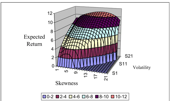
.u . When they exist, this equation may be re-expressed in term of the expected return vector, the covariance matrix and λ the vector of skewness coefficients. A sketch of the efficient surface is shown in Figure 2. The equations that generate it are essentially the same as those in A&S and are summarised in Appendix B.
Figure 2 about here
It is well known that the moment generating function does not exist for random variables that follow Student distributions. Consequently, when asset returns follow the MEST distribution, the use of the negative exponential function is not available to expected utility maximisers. However, the implication of the regularity conditions is that utility functions may be constructed which are continuous and for which the first two derivatives exist. For given values of θ1,2 portfolio selection may be carried out using quadratic programming.
6. Concluding Remarks
The properties of the market model may be summarised as follows. Under the MEST distribution, there are three forms of market model. First, when the market portfolio does not possess skewness, the market model is non-linear in market portfolio return rp. However, the non-linearity vanishes as the degrees of freedom increase. In this case, the sensitivity of asset returns to the market is similar to the conventional beta. Secondly, if the market portfolio does possess skewness, then the market model is always non-linear and the sensitivity of asset returns to the market is not equivalent to beta. Finally, in the case where conditional skewness equals zero, the market model is always linear and the sensitivity, as above, is similar to beta. The conditional variance of asset returns is time varying and is dependent on the squared deviation of market portfolio return from its location parameter.
Although there are some restrictions on the choice of utility function, all expected utility maximisers will select portfolios from an efficient surface, which is the analogue of the familiar mean-variance frontier.
The treatment of skewness depends on the use of a single skewness variable. A development of this work will be to extend the model so that multiple skewness shocks may be incorporated. As already noted, this extension is expected to be of mainly theoretical interest, since the practical difficulties associated with such a model are substantial.
Acknowledgements
This is a revised version of a paper originally presented at the Multi-moment Capital Asset Pricing Conference held in Paris in April 2002. It benefitted from the comments of several conference participants, with particular thanks to Renato Flores and Steve Satchell as well as to Emmanuel Jurczenko and Bertrand Maillet, the organisers of the meeting. More recently this work has been presented at the workshop on skew-elliptical distributions held in Bertinoro, Italy in April 2008 organised by Adelchi Azzalini and Antonella Capitanio and at a seminar at the University of Padua. Both this paper and intended future developments have been greatly assisted by the comments of participants at the workshop and at the seminar. I am very grateful to the two organisers of the workshop for the opportunity to participate in the meeting and for their helpful guidance. I am also grateful to Marc Genton for a pre-print of his 2008 paper with Reinaldo Arellano-Valle. Finally, this paper has benefitted greatly from the comments of the anonymous referee and from recent correspondence from Professor Azzalini. Remaining errors and shortcomings are mine alone.
Appendices
A – The Conditional Expected Value
Three cases of the conditional distribution are considered: (i) λ1 =0, (ii) at least one element of λ1is non-zero and (iii) the special case λ2|1 =0.
Case 1: λ1 = 0
(
|)
1( 1 1) 2(
) (
)
( ) 11 21 2 2 12 = + τ+ − − + υ1+Q1 υ υ+n1 ξυ+n1 Ξ
E R r µ λ Σ Σ r µ λ ,
where ξυ
( )
is as defined above and Ξ=τ υ(
1+Q1 υ) (
υ+n1)
. Using the formulae in Section 3.7 for the expected value of R2 and noting that, for υ>1, E( )
R1 = µ1, the above conditional expectation may be written as(
)
E( )
{
E( )
}
{
υ(
1 Q υ) (
υ n)
ξ( )
ξ( )
τ}
E = + − − + + 1 + 1 υ+n1 Ξ − υ
2 1 1 1 11 21 2 1
2 |r R Σ Σ r R λ
R .
Since λ1 =0, −1 =Β 11 21Σ
Σ is the n2×n1 matrix of theoretical coefficients for the multivariate regression of R2on R1. The regression above has two components. The first is linear in the conditioning vector r1. The matrix Βhas almost the same interpretation as in regression1. The residual term
(
1 Q υ) (
υ n)
ξ( )
ξ( )
τυ 1 1 υ n υ
1 Ξ −
+ +
=
∆ + ,
is non-linear in r1. As the degree of freedom parameter υ increases without limit, 0
→
∆ with probability one. The conditional expectation therefore has a limiting linear form as υ→∞. Taking expectations gives E
( )
∆ =02 for all υ. The term ∆acts like a residual; it contributes to variability, but not to unconditional expected return. The implication is that the use of OLS would result in an unbiased estimator of
Β, but that the results would be inefficient.
Case 2: At least one element of λ1 not equal to 0
When λ1 ≠0, that is when one or more of the conditioning variables possesses skewness, the conditional expected value may be written as
(
2 1)
( )
2{
1( )
1}
2 ~ ~ ~|r = R +Br − R +∆λ
R E E
E
where:
(
1) (
)
( ) ( ) 1 .~ , 1 ~ , ) )( ( ~ 1 1 11 1 1 | 2 1 1 1 1 11 1 1 1 11 21 2 2 1 1 1 11 1 2 21
1 λ λ
λ λ λ λ λ λ λ λ λ − + − − − + τ ξ − τ ξ + + = ∆ + − = + + = Σ Σ Σ Σ Σ Σ B T υ n υ T T T n υ υ Q υ
The matrix B~ still measures the linear sensitivity of the elements of R2 to elements of r1. However, the interpretation of B~ is different. A second difference is that ∆~
1 It has the same interpretation as long as υ> 2. For smaller values of υ, a slightly different
interpretation of B is needed, although it still determines the sensitivity of elements of R2 to elements
does not tend to zero as the degrees of freedom increase, although it is of course true that E
( )
∆~ =0 . Thus, even in the limiting case of multivariate skew-normality, the regression model is non-linear.Case 3: λ2|1 = 0
A model that is exactly linear with respect to R1 arises when λ2|1 = ~λ2 =0. In this case, the conditional expected value of R2 given r1 is
(
R2 |r1)
E( )
R2 B{
r1 E( )
R1}
E = + − .
Where B is as defined above. Although this is a special case, it merits a comment. The vector variables R1 and R2 have a MEST distribution both jointly and individually. When λ2|1 = ~λ2 =0, the conditional distribution of R2 given that
1 1 r
R = is the elliptically symmetric modification of the multivariate Student in Section 3.2. The interpretation of this result is that the conditioning variable
1
R accounts for all the skewness in R2. In view of the linear transformations property in Section 3.1, this raises the possibility of creating linear combinations of R which account for the skewness present in all variables. Conversely, it raises the possibility that a linear regression model may conceal skewness in the dependent or independent variables or in both.
B – Efficient Set Mathematics
For given values of θ1 and θ2, the solution to the standard efficient set problem
(
)
{
}
s. .t 1 Emax wT Tw =
w u R 1 is the set of equations
(
Σ+λλT)
w−θ1µ−θ2λ-ζ1=0,where ζ is the Lagrange multiplier of the budget constraint, which is the n-vectors of ones, 1. A&S show that this leads to an efficient surface as follows. Let the solution be w*and define
λ
µ T T
T
E*=w ,V*=w Σw,S*=w .
Some algebra gives the following
(
)
(
)
{
(
)
1}
2 2 2
1 2 0 1 1
2 0
0 γ S* γ /γ α γ γ V* α S* γ γ
α *
E − = − + − − − − ,
(
)
(
)
(
)
, . , , 1 , , 1 1 2 1 1 1 1 1 1 1 1 1 0 1 2 1 1 1 1 1 1 1 0 1 Σ 1 1 Σ 1 Σ 1 Σ 11 Σ Σ 1 Σ 1 Σ 11 Σ Σ 1 Σ 1 1 Σ 1 Σ 11 Σ Σ 1 Σ 1 1 Σ − − − − − − − − − − − − − − − − − = γ − = γ − = γ = α − = α = α T T T T T T T T T T T T T T λ λ λ λ µ µ µ µ ReferencesAdcock, C. J. (2005)Exploiting Skewness To Build An Optimal Hedge Fund With A Currency Overlay, The European Journal of Finance, 11, 445-462.
Adcock, C. J. (2007) Extensions of Stein’s Lemma for the Skew-normal Distribution, Communications in Statistics – Theory and Methods, 36, 1661-1672.
Adcock, C. J. (2008) Extensions of Stein’s and Siegel’s Lemmas for the Skew-Student Distribution, Working Paper.
Adcock, C. J. & K. Shutes (2001) Portfolio Selection Based on the Multivariate Skew-Normal Distribution in Financial Modelling (A Skulimowski, Editor), Krakow , Progress and Business Publishers.
Aparicio, F. & J. Estrada (2000) Empirical distributions of stock returns: European Securities markets, European Journal of Finance, 7, 1-21.
Arrellano-Valle, R. B. and A. Azzalini (2006) On the unification of families of skew-normal distributions, Scand. J. Statist., 33, 561-574.
Arellano-Valle, R. B., M. D. Branco & M. G. Genton (2006). A unified view on skewed distributions arising from selections. Canad. J. Statist., 34, 581–601. Arellano-Valle, R. B. and M. G. Genton (2005). On fundamental skew distributions,
J. Multivariate Analysis, 96, 93-116.
Arrellano-Valle, R. B. & M . G. Genton (2008) Multivariate Extended Skew-t Distributions and Related Families with Applications, Technical Report # 080628, Department of Econometrics, University of Geneva
Azzalini, A. (1985) A Class of Distributions Which Includes The Normal Ones, Scand. J. Statist, 12, 171-178.
Azzalini, A. (1986) Further Results on a Class of Distributions Which Includes The Normal Ones, Statistica, 46, 199-208.
Azzalini, A. & A. Capitanio (2003) Distributions Generated by Perturbation of Symmetry With Emphasis on a Multivariate Skew t Distribution, J Roy Statist. Soc Series B, 65, 367–389.
Azzalini, A. & A. Dalla-Valle (1996) The Multivariate Skew-normal Distribution, Biometrika, 83, 715-726.
Azzalini, A. & M. G. Genton (2008) Robust Likelihood Methods Based on the Skew-t and Related Distributions, International Statistical Review (2008), 76, 106– 129
Bauwens, L. & S. Laurent (2005) A New Class of Multivariate Skew Densities, With Applications to GARCH Models, Journal of Business and Economic Statistics, 23, 346-354.
Bernardo, J. M. & A. F. M. Smith (1994) Bayesian Theory, New York, John Wiley and Sons Inc.
Branco, M. D. and D. K. Dey (2001) A general class of multivariate skew-elliptical distributions, J. Multivariate Anal., 79, 99-113.
Cherubini, U., E. Luciano, & W. Vecchiato (2004) Copula Methods in Finance. New York, John Wiley.
Fama, E. (1970) Efficient Capital Markets: A Review of Theory and Empirical Work, Journal of Finance, 25, 383-417.
Fang, K.-T., S. Kotz & K.-W. Ng, (1990). Symmetric multivariate and related distributions. Monographs on Statistics and Applied Probability, Vol. 36. London, Chapman & Hall, Ltd.
Genton, M.G. (2004) Skew-Elliptical Distributions and Their Applications: A Journey Beyond Normality. Edited volume, Boca Raton, Chapman & Hall/CRC Press. Gonzàlez-Farías, G., A. Dominguez-Molína & A. K. Gupta (2004) Additive
Properties of skew normal random vectors, Journal of Statistical Planning and Inference, 126, 521-534.
Johnson, N. L. & S. Kotz (1972) Distributions in Statistics, Continuous Multivariate Distributions, New York, John Wiley and Sons Inc.
Jones, M. C. (2001) Multivariate t and Beta Distributions Associated with the Multivariate F Distribution, Metrika, 54, 215-231.
Jones, M. C. (2002) Marginal Replacement in Multivariate Densities, with Application to Skewing Spherically Symmetric Distributions, Journal of Multivariate Analysis, 81, 85-99.
Jones, M. C. & M. J. Faddy (2003 A skew Extension of the t Distribution, with Applications, J Roy Statist. Soc Series B, 65, 159-174.
Harvey, C. R., J. C. Leichty, M. W. Leichty & P. Muller (2004) Portfolio Selection With Higher Moments, Working Paper.
Horrace, W. C. (2005). Some results on the multivariate truncated normal distribution. J. Multivariate Anal. 94, 209–221.
Kallberg, J. G. & W. T. Ziemba (1983) Comparison of Alternative Functions in Portfolio Selection Problems, Management Science, 11, 1257 – 1276.
Landsman, Z. (2006) On the generalization of Stein’s Lemma for elliptical class of distributions, Statistics & Probability Letters, 76, 1012–1016
Landsman, Z. & J. Nešlehová (2008) Stein’s Lemma for elliptical random vectors, Journal of Multivariate Analysis, 99, 912 – 927
Liu, J. S. (1994) Siegel’s Formula via Stein’s Identities, Statistics and Probability Letters, 21, 247-251.
McDonald, J. B. & Y. J. Xu (1995) A Generalization of the Beta Distribution with Applications, Journal of Econometrics, 66, 133-152.
Meucci, A. (2006) Beyond Black-Littermann: views on non-normal markets, Risk, February 2006, 87-92.
Praetz, P. (1972) The Distribution of Share Price Changes, Journal of Business, 45, 49-55.
Sahu, S. K., D. K. Dey & M. D. Branco (2003) A New Class of Multivariate Skew Distributions With Applications to Bayesian Regression Models, Canad. J. Statist., 31, 129-150.
Stein, C. (1981) Estimation of the Mean of a Multivariate Normal Distribution, Annals of Statistics, 9, 1135-1151.
Theodossiou, P. (1998) Financial Data and the Skewed Generalized T Distribution, Management Science, 44, 1650-1661.
Figure 1 - A Sketch of Conditional Expected Value
-1 -0.5 0 0.5 1 1.5 2
-0.5 -0.4 -0.3 -0.2 -0.1 0.0 0.1 0.2 0.3 0.4 0.5
Market return
E[R|Market return]
lambda = 0 lambda = 0.1 lambda = 0.5 lambda = 1.0
Figure 2 – Sketch of the Mean-Variance-Skewness Efficient Surface
1 5 9
13 17
21
S1 S11
S21 0
2 4 6 8 10 12
Expected Return
Skewness
Volatility
[image:19.595.119.480.429.641.2]