A structure-preserving matrix method for the deconvolution of two Bernstein basis polynomials

This is a repository copy of A structure-preserving matrix method for the deconvolution of two Bernstein basis polynomials.

White Rose Research Online URL for this paper: http://eprints.whiterose.ac.uk/91525/

Version: Accepted Version

Article:

Winkler, J.R. and Yang, N. (2014) A structure-preserving matrix method for the

deconvolution of two Bernstein basis polynomials. Computer Aided Geometric Design, 31 (6). 317 - 328. ISSN 0167-8396

https://doi.org/10.1016/j.cagd.2014.02.009

Reuse

Unless indicated otherwise, fulltext items are protected by copyright with all rights reserved. The copyright exception in section 29 of the Copyright, Designs and Patents Act 1988 allows the making of a single copy solely for the purpose of non-commercial research or private study within the limits of fair dealing. The publisher or other rights-holder may allow further reproduction and re-use of this version - refer to the White Rose Research Online record for this item. Where records identify the publisher as the copyright holder, users can verify any specific terms of use on the publisher’s website.

Takedown

If you consider content in White Rose Research Online to be in breach of UK law, please notify us by

A structure-preserving matrix method for the

deconvolution of two Bernstein basis

polynomials

Joab R. Winkler,

Ning Yang

a_{Department of Computer Science, The University of Sheffield, Regent Court,} 211 Portobello, Sheffield S1 4DP, United Kingdom

[email protected],[email protected]

Abstract

This paper describes the application of a structure-preserving matrix method to the deconvolution of two Bernstein basis polynomials. Specifically, the deconvolution ˆ

h/fˆ yields a polynomial ˆg provided the exact polynomial ˆf is a divisor of the exact polynomial ˆh and all computations are performed symbolically. In practical situations, however, inexact forms, h and f of, respectively, ˆh and ˆf are specified, in which case g = h/f is a rational function and not a polynomial. The simplest method to calculate the coefficients ofgis the least squares minimisation of an over-determined system of linear equations in which the coefficient matrix is Tœplitz, but the solution is a polynomial approximation of a rational function. It is shown in this paper that an improved result forg is obtained when the Tœpliz structure of the coefficient matrix is preserved, that is, a structure-preserving matrix method is used. In particular, this method guarantees that a polynomial solution to the deconvolution h/f is obtained, and thus an essential property of the theoretically exact solution is retained in the computed solution. Computational examples that show the improvement in the solution obtained from the structure-preserving matrix method with respect to the least squares solution are presented.

Key words: Polynomial deconvolution; Bernstein basis polynomials; structure-preserving matrix methods

1 Introduction

developed [3,4], and this paper considers the deconvolution of two Bernstein basis polynomialshandf, that is, the computation of the polynomialg =h/f. Ifh= ˆh andf = ˆf where ˆhand ˆf are the exact forms ofhand f respectively,

ˆ

f is an exact divisor of ˆh, and all computations are performed symbolically, then ˆg = ˆh/fˆis a polynomial. In practical problems, however, the polynomials h and f are inexact, in which case g = h/f is a rational function and not a polynomial. It is shown in this paper that in this circumstance, a polynomial is returned when a structure-preserving matrix method is used to compute g. This solution must be compared with the simplest solution, that is, the least squares (LS) solution of an over-determined set of linear equations, in which case a polynomial approximation of a rational function is returned.

The approximation of a rational function by a polynomial may be adequate in some applications, but other applications may require that the algorithm for polynomial deconvolution return a polynomial, and not an approximation of a polynomial. The requirement that a polynomial be returned arises in the computation of multiple roots of a polynomial because the algorithm includes a series of deconvolutions in which the denominator polynomial is an exact divisor of the numerator polynomial [8]. The discussion above shows that if the polynomials are subject to error and/or the computations are performed in finite precision arithmetic, it cannot be guaranteed that the result of each deconvolution is a polynomial. In this circumstance, the algorithm returns in-correct results or fails, and it is shown in this paper that a structure-preserving matrix method returns polynomial solutions to these deconvolutions, which is, as noted above, essential for the computation of multiple roots of a polynomial.

The deconvolution of two Bernstein basis polynomials is considered in Section 2. It is shown that the problem can be cast as the computation of the vector ˆ

g, which stores the coefficients of ˆg, from the equation,

D−1_{T( ˆf)ˆg= ˆh, (1)}

where D−1 _{is a diagonal matrix of combinatorial factors, T( ˆf) is a Tœplitz}

matrix whose non-zero entries are the coefficients of ˆf, and ˆh stores the coef-ficients of ˆh. The Tœplitz structure of T( ˆf) is retained when inexact polyno-mials hand f are specified, but h, the vector that contains the coefficients of h, does not lie in the column space ofD−1_{T(f) in this circumstance, and thus}

(1) is replaced by

D−1_{T(f)g≈h. (2)}

The approximation in (2) implies that a computed solutionw has a non-zero error, kD−1_{T(f)w−hk > 0, from which it follows that the entries of w are}

It is shown in Section 3 that if the Tœplitz structure of T(f) is retained in the computations, that is, a structure-preserving matrix method is used, an exact polynomial, and not a polynomial approximation of a rational function, is returned when an approximate solution of (2) is computed.

The application of a structure-preserving matrix method to the deconvolution of two Bernstein basis polynomials is considered in Section 4. This method requires the iterative solution of a non-linear equation, and the condition for its convergence is discussed in Section 5. Section 6 contains two examples that compare the solutions obtained from the method of LS with the solutions ob-tained from a structure-preserving matrix method. The solutions are discussed in Section 7, and Section 8 contains a summary of the paper.

2 The deconvolution of two Bernstein polynomials

This section considers the deconvolution of two Bernstein polynomials and it is shown it can be considered in the matrix form (1).

Let ˆf(y),gˆ(y) and ˆh(y) be Bernstein polynomials of degrees m, n and m+n respectively,

ˆ f(y) =

m

X

i=0

ˆ ai

m i

!

(1−y)m−i_yi_{, (3)}

ˆ g(y) =

n

X

i=0

ˆ_bi n i

!

(1−y)n−i_yi_{, (4)}

ˆ h(y) =

m+n

X

i=0

ˆ ci

m+n i

!

(1−y)m+n−iyi. (5)

It follows from (3) and (4) that the coefficients ˆci in (5) are given by

ˆ ck=

min(m,k)

X

i=max(0,k−n)

ˆ ai

_m

i

ˆ_{bk−i n}

k−i

_m+n

k

, k = 0, . . . , m+n,

which can be written in matrix form as

D−1T( ˆf)

ˆ

b= ˆc, (6)

D−1 = diag

1

(m+n 0 )

1

(m+n 1 )

· · · 1

( m+n m+n−1)

1

(m+n m+n)

∈R(m+n+1)×(m+n+1),

T =T( ˆf)∈R(m+n+1)×(n+1), ˆb∈Rn+1, ˆc∈Rm+n+1 and

T =                          ˆ a0 _m 0 ˆ a1 _m 1 ˆ a0 _m 0 .. . ˆa1

_m

1

. ..

... ... ... ˆa0

_m 0 ˆ am _m m ..

. . .. ˆa1

_m 1 ˆ am _m m . .. ... . .. ... ˆ am _m m                         

, bˆ =

              ˆ b0 _n 0 ˆ b1 _n 1 .. . ... ˆ_bnn

n              

, ˆc=

              ˆ c0 ˆ c1 .. . ... ˆ cm+n

              .

Previous work [11,12] has shown it is numerically advantageous to express ˆb

as the product of a diagonal matrix Q ∈R(n+1)×(n+1) _{and a vector ˆp∈ R}n+1

of the coefficients ˆbi,

ˆ

b=Qpˆ, Q= diag

_n 0 n 1

· · · n_n

, pˆ =

ˆ_b0 ˆ_{b1 · · ·} ˆ_bnT _,

and thus (6) can be written as

D−1_{T( ˆf)Qpˆ = ˆc, (7)}

where the coefficient matrix is of order (m +n+ 1)×(n+ 1). It is better to calculate the coefficients of ˆg(y) from (7) than from (6) because numerous experiments showed that

κ

D−1T( ˆf)Q

< κ

D−1T( ˆf)

,

where κ(X) denotes the condition number of X. It therefore follows that (7) is more stable than (6), and thus improved solutions are expected from (7).

normalisation of the entries in the right hand side vector, by their geometric means yield significantly improved results. The geometric mean of the terms that contain the coefficients of ˆf in D−1_{T( ˆf)Q is [12]}

λ=

Qm

i=0

ˆai

_m

i

1

m+1Qn

k=0

_n

k

1

n+1

(Qm

i=0Pi)

1 (n+1)(m+1)

, (8)

where

Pi = i+n

Y

j=i

m+n j

!

, i= 0, . . . , m,

and thus the normalised form of ˆf(y) is

¯ f(y) =

m

X

i=0

¯ ai

m i

!

(1−y)m−iyi, ¯ai =

ˆ ai

λ. (9)

The normalised form of ˆh(y) is

¯ h(y) =

m+n

X

i=0

¯ ci

m+n i

!

(1−y)m+n−i_yi_{, ¯c} i =

ˆ ci

µ, (10)

where the geometric mean µof the coefficients ˆci is

µ=

m+n

Y

i=0

|ˆci|

!_m+1_n+1

. (11)

It therefore follows from (9) and (10) that (7) becomes

D−1T( ¯f)Q

¯

p= ¯c, (12)

where ¯c∈Rm+n+1 _{and ¯p∈R}n+1 _{are, respectively,}

¯

c=

¯

c0 ¯c1 · · · ¯cm+n

T

and p¯ =

¯_b0 ¯_{b1 · · ·} ¯_bnT_,

¯ g(y) =

n

X

i=0

¯ bi

n i

!

(1−y)n−i_yi_.

The normalisation of the coefficients of ˆf(y) retains the Tœplitz structure of T, but the inclusion of the diagonal matricesD−1 _{andQimplies that the}

coef-ficient matrix in (12) is not Tœplitz, but it is still structured. It is appropriate to consider, therefore, a structure-preserving matrix method for the solution of (12), and this issue is addressed in the next section.

3 A structure-preserving matrix method

This section considers the application of a structure-preserving matrix method to the solution of (12), and the difference between the solution obtained using this method, and the solution obtained by solving a LS problem, is described.

If exact polynomials are considered and all computations are performed in infinite precision arithmetic, the coefficients of ¯g can be computed from the LS solution of (12),

¯

p=

D−1_{T( ¯f)Q}†_{¯c, A}† _{= (A}T

A)−1_AT

,

and the error is zero. The pseudo-inverseA†_{of a matrixAshould be computed} from the singular value decomposition (SVD) of A and not from the SVD USVT _ofA† _{because this can lead to large errors, such that USV}T _6=A†_.

If the inexact polynomials f(y) and h(y) are considered, then (12) is replaced by an approximate equation whose LS solution defines the coefficients of a polynomial that is an approximation of a rational function. This is the sim-plest method of computing the coefficients of ¯g(y), but it fails to consider the structure of the coefficient matrix. Sincef(y), g(y) andh(y) are inexact forms of ˆf(y),gˆ(y) and ˆh(y) respectively, they are given by

f(y) = ˆf(y) +δfˆ(y) =

m

X

i=0 ai

m i

!

(1−y)m−i_yi_{, (13)}

g(y) = ˆg(y) +δgˆ(y) =

n

X

i=0 bi

n i

!

(1−y)n−iyi,

h(y) = ˆh(y) +δˆh(y) =

m+n

X

j=0 cj

m+n j

!

(1−y)m+n−j_yj_{, (14)}

ai = ˆai+δˆai and cj = ˆcj +δˆcj, (15)

and normalisation of the coefficients ai and cj by, respectively, the geometric

meansλ and µ, which are defined in (8) and (11), is implicitly included. This normalisation by the geometric means of the coefficients of f(y) and g(y) follows from the discussion in Section 2.

It follows from (12) that it is necessary to compute the LS solution of

D−1_T(f)Q

p≈c, (16)

where

p=

b0 b1 · · · bn

T

and c=

c0 c1 · · · cm+n

T

.

The vector c does not lie in the column space of D−1_{T(f)Q, but the}

ap-proximation (16) can be transformed to an equation by perturbing T(f) by a Tœplitz matrix B(z) that has the same structure as T(f), and perturbing

c by a vector t. A structure-preserving matrix method yields, therefore, a polynomial solution to the deconvolution problem because (16) is replaced by

D−1_{(T(f) +B(z))Qp=c+t, (17)}

where the entries of B(z) and t are the coefficients of the polynomials s(y) and e(y) respectively,

s(y) =

m

X

i=0 zi

m i

!

(1−y)m−iyi, (18)

and

e(y) =

m+n

X

i=0 ti

m+n i

!

(1−y)m+n−i_yi_{, (19)}

B(z) =                          z0 _m 0 z1 _m 1 z0 _m 0 .. . z1

_m

1

. ..

... ... ... z0

_m 0 zm _m m ..

. . .. z1

_m 1 zm _m m . .. ... . .. .._. zm _m m                         

, t=

              t0 t1 ... ... tm+n

              .

If the matrix B(z) and vectort are chosen such that c+t lies in the column space of D−1_{(T(f) +B(z))Q, then (17) has an exact solution, and thus the}

solution vector p contains the coefficients of the polynomial formed from the deconvolution,

h(y) +e(y) f(y) +s(y) =

Pm+n

i=0 (ci+ti)

_m+n

i

(1−y)m+n−i_yi

Pm

i=0(ai+zi)

_m

i

(1−y)m−i_yi . (20)

An infinite number of pairs of polynomials (s(y), e(y)) satisfy (17), but it is desired to compute the coefficients zi and ti of minimum magnitude, that is,

the solution of (17) that is nearest the solution defined by the given inexact data is sought. This is expressed mathematically as an LS minimisation with an equality constraint, the LSE problem,

min kzk2+ktk2 such that

D−1_{(T(f) +B(z))Qp=c+t, (21)}

where k·k=k·k₂,

z=

z0 z1 · · · zm

T

and z =

z0, z1, · · · , zm

. (22)

4 The method of STLN for the deconvolution of two polynomials

This section considers the application of the method of structured total least norm (STLN) [6] to the deconvolution h/f, such that the result is a polyno-mial and not a rational function. This method is therefore used to obtain the solution of (21).

The residual associated with an approximate solution (z,p,t) of (17) is

r(z,p,t) = (c+t)−D−1_{(T(f) +B(z))Q}

p, (23)

and thus

˜

r:=r(z+δz,p+δp,t+δt) = (c+ (t+δt))−

D−1_{(T(f) +B(z+δz))Q(p+δp).}

It therefore follows that, to first order,

˜

r=r(z,p,t) +δt−

D−1_{(T +B)Qδp− D}−1 Xm

i=0 ∂B ∂zi

δzi

!

Q

!

p,

(24)

where the last term on the right hand side represents the polynomial multi-plicationδs(y)g(y), and s(y) is defined in (18). The simplification of this term requires that the polynomial multiplication

g(y)s(y) =

n

X

i=0 bi

n i

!

(1−y)n−i

yi

! _m X

i=0 zi

m i

!

(1−y)m−i

yi

!

,

which can also be expressed as

s(y)g(y) =

m

X

i=0 zi

m i

!

(1−y)m−i_yi

! _n X

i=0 bi

n i

!

(1−y)n−i_yi

!

,

be considered. These polynomial multiplications can be expressed in matrix forms as, respectively,

D−1Y(p)Rz and D−1B(z)Qp, (25)

p=

b0, b1, · · ·, bn

and R= diag

_m 0 m 1

· · · m_m

.

It therefore follows from (25) that

(Y R)z= (BQ)p,

and the differentiation of both sides of this equation with respect to zyields

(Y R)δz=

m X i=0 ∂B ∂zi δzi !

Qp,

and thus (24) simplifies to

˜

r=r(z,p,t) +δt−

D−1_{(T(f) +B(z))Qδp−(D}−1_{Y R)δz. (26)}

The jth iteration in the Newton-Raphson method for the calculation of z,p

and t is obtained from (26),

Hz Hp Ht

(j)        δz δp δt       

(j)

=r(j), (27)

where r(j)_=r(j)_(z,p,t),

Hz=D−1Y R ∈R(m+n+1)×(m+1),

Hp=D−1(T +B)Q∈R(m+n+1)×(n+1),

Ht=−I ∈R(m+n+1)×(m+n+1),

and the values of z,p and tat the jth iteration are

       z p t       

(j)

=        z p t       

(j−1)

+        δz δp δt       

(j)

,        z p t        (0) =        0 p₀ 0        .

p₀ = arg min w

D−1T(f)Qw−c

. (28)

Equation (27) is of the form

C(j)_δy(j) _=q(j)_{, q}(j) _=r(j) _∈

Rm+n+1, (29)

where C(j) _∈R(m+n+1)×(2m+2n+3)_{, δy}(j)_∈R2m+2n+3_{, and}

C(j)=

Hz Hp Ht

(j)

, δy(j)=

       δz δp δt       

(j)

, y(j)=y(j−1) +δy(j). (30)

It follows from (21) that, of all the solutions that satisfy the constraint equa-tion, the solution that is nearest the LS solution defined by the given inexact data is required. The function to be minimised is therefore

      

z(j)−z(0) p(j)_−p

0

t(j)−t(0)

       =       

z(j−1)_+δz(j)

p(j−1)_+δp(j)_−p 0

t(j−1)+δt(j)

       := δy

(j)_−w(j−1)

, (31)

where δy(j) _{is defined in (30), δy}(0) _=w(0) _{=0 and}

w(j−1) =−y(j−1)−y(0)=−       

z(j−1)

p(j−1)−p₀ t(j−1)

      

∈R2m+2n+3. (32)

The minimisation of (31) subject to (29) yields the LSE problem,

min

δy(j)

δy

(j)_−w(j−1)

subject to C

(j)_δy(j)_=q(j)_{, (33)}

which can be solved, at each iteration, by the QR decomposition [5], where C(j)_,q(j) _{and w}(j−1) _{are updated between successive iterations.}

Algorithm 1: Deconvolution of two Bernstein polynomials

Input Inexact polynomials f and h, which are of degrees m and m+n re-spectively.

Output The polynomial g =h/f.

Begin

(1) Preprocess f and h as shown in Section 2. (2) % Initialise the data

(a) Setz=z(0) =0, which yields B =B(0) _{= 0, and t=t}(0) _=0.

(b) Calculate T, Y(0) _{and the initial value p}

0 of p, which is defined in

(28). Calculate r(0), the initial value of the residual,

q(0) =r(0) =rz(0)=0,p₀,t(0) =0=c−D−1T(f)Qp₀. (c) Define C(0) _{and set w}(0) _=0.

(3) % Use the QR decomposition to solve the LSE problem at each iteration.

Set j = 0. % Initialise the iteration counter

repeat

(a) Setj =j+ 1. % Increment the iteration counter (b) Compute the QR decomposition ofC(j−1)T

,

C(j−1)T

= (QR)(j−1) =



Q 

 

R1

0



 





(j−1) .

(c) Setw(₁j−1) =

R−T

1 q

(j−1)

.

(d) Partition Q(j−1) _as

Q(j−1) ₌ Q1 Q2

(j−1)

,

whereQ(₁j−1) ∈R(2m+2n+3)×(m+n+1) _{and Q}(j−1)

2 ∈R(2m+2n+3)×(m+n+2).

(e) Compute z(₁j−1) =

QT

2w

(j−1)

where w(j−1) _{is defined in (32).}

(f) Compute the solution

δy(j)=



Q 

 

w1

z1



 





(g) Setz(j)_=z(j−1)_+δz(j)_,p(j) _=p(j−1)_+δp(j) _andt(j) _=t(j−1)_+δt(j)_,

and thus calculatey(j) and w(j).

(h) UpdateB(j)_andY(j)_{, and thereforeC}(j)_{, fromz}(j)_andp(j)_{. Compute}

the residualq(j)_=r(j)

z(j)_,p(j)_,t(j)

from (23),

r(j)z(j),p(j),t(j)=c+t(j)−D−1T +B(j)Qp(j).

until kr

(j)_k

kc+t(j)_)k ≤10 −12

End

Optimality conditions for the method of STLN, its formulation for the 1- and

∞-norms, and its relation to the Newton-Raphson iteration, are considered in [6]. The method can be extended to non-linear structures in the coefficient matrix and/or right hand side vector, which yields the method of structured non-linear total least norm [7]. This method has been used for the computation of a structured low rank approximation of the Sylvester resultant matrix [9].

5 Convergence analysis

This section considers the convergence of Algorithm 1 for the iterative solution of the LSE problem, which is defined in (21). It follows from steps (3c)-(3f) of this algorithm, and (32), that thejth iteration of this LSE problem yields

δy(j)=



Q 

 

R−T

1

0



 q+Q



 

0

z1



 





(j−1)

=



Q 

 

R−T

1

0



 q+

Q1 Q2



 

0

QT

2



 w





(j−1)

=Q1R1−Tq

(j−1)

+Q2QT2

(j−1)

−y(j−1)+y(0). It follows from (30) that Algorithm 1 converges if

lim

j→∞

y

(j)_−y(j−1) = lim

j→∞

δy

(j)

= lim

j→∞

Q2QT2

(j−1)

y(0)−y(j−1)+Q1R−1Tq

(j−1)

and thus the convergence of (33) is dependent on the matrices and vectors at each iteration, and itsa priori determination is therefore difficult. Compu-tational experiments showed, however, that convergence is achieved in fewer than 5 iterations, even for high degree polynomials that are corrupted by noise and have multiple roots.

6 Examples

This section contains two examples that illustrate the application of the method of STLN to the computation of g =h/f, and the solution of each example is compared with the LS solution of (16). Also, it was stated in Section 2 that it is numerically advantageous to include the diagonal matrix Q of combina-torial factors in the coefficient matrix, and this is confirmed numerically by including the solutions obtained when (16) is written as

D−1_{T(f)b≈c, b=Qp. (34)}

Three error measures and two condition numbers were computed for each example:

The error r1 between the theoretically exact solution, that is, the coefficients

of gˆ(y), and the solution of the LSE problem (33). If this solution defines the polynomialg1(y), then the forward error in the coefficients of g1(y) is

r1 =

kg₁−gˆk

kˆgk . (35)

The error r2 between the theoretically exact solution and the LS solution of

(16).If this solution defines the polynomialg2(y), then the forward error in

the coefficients ofg2(y) is

r2 =

kg₂−gˆk

kˆgk . (36)

The errorr3 in the satisfaction of the constraint equation in the LSE problem.

The residual of the computed solution of the constraint is, from (23),

r3 =

kr(z,p,t)k

kc+tk . (37)

Condition number 1:The condition numberκC(j)_{of the coefficient matrix}

iterative procedure, forQincluded in the coefficient matrix, andQincluded in the solution vector.

Condition number 2: The condition numbers κ(D−1_{T(f)Q) andκ(D}−1_T(f))

of the LS problem, forQ included in the coefficient matrix and Qincluded in the solution vector, respectively.

Also, the number of iterationsN required for the solution of the LSE problem was recorded.

Noise was added in the componentwise sense to the coefficients of ˆf(y) and ˆ

h(y), and it therefore follows from (13) and (14) that the coefficients of the polynomials δfˆ(y) andδˆh(y) are, respectively,

δaˆi =εriaˆi, i= 0, . . . , m; δˆcj =εrjcˆj, j = 0, . . . , m+n, (38)

where ri and rj are uniformly distributed random variables in the interval

[−1,1], and ε is the reciprocal of the upper bound of the componentwise signal-to-noise ratio. The normwise error models follow easily from these com-ponentwise error models,

kδaˆk ≤εkaˆk and kδˆck ≤εkˆck, (39)

and thus ε is also the upper bound of the reciprocal of the normwise signal-to-noise ratio.

Example 6.1 Noise with componentwise signal-to-noise ratio 108 was added to the coefficients of the Bernstein forms of the exact polynomials,

ˆ

f(y) = (y−0.30)5(y−0.70)4(y−1.40)5(y−7.00)6, and

ˆ

h(y) = (y−0.30)8(y−0.70)7(y−1.40)8(y−7.00)6(y+ 1.80)3×

(y+ 0.90)4,

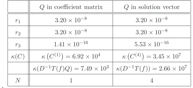
and these inexact polynomials were then normalised, thereby obtaining the polynomialsf(y) andh(y), which are defined in (13) and (14). The results are shown in Table 1 and it is seen that r1 = r2, and thus the relative errors of

the solutions in the LS and LSE problems are equal. The errorr3 is

approxi-mately equal to 10−16_{, and it therefore follows from (37) and the discussion in}

Section 3 that the computed solution is a polynomial, and not a polynomial approximation of a rational function. This value of r3 must be compared with

thus the difference between the solutions from the LS and LSE problems is clear.

Table 1 shows that the inclusion of Q in the coefficient matrix causes a re-duction of about three orders of magnitude in κC(j)

with respect to its value when Q is included in the solution vector, as shown in (34), which is in accord with the results in [11,12]. The table also shows that, for Q included in the coefficient matrix,κC(j) _{is about one order of magnitude larger than}

the condition number of D−1_{T(f)Q, which is the coefficient matrix of (16).}

Also, one iteration is required for the convergence of the LSE problem when Q is included in the coefficient matrix, but four iterations are required for

convergence when Q is included in the solution vector.

Q in coefficient matrix Qin solution vector

r1 3.20×10−8 3.20×10−8 r2 3.20×10−8 3.20×10−8 r3 1.41×10−16 5.53×10−16 κ(C) κ C(1)

= 6.92×104 _{κ C}(4)

= 3.45×107 κ(D−1_{T(f)Q) = 7.49×10}3 _κ(D−1_{T(f)) = 2.66×10}7

N 1 4

Table 1

The results of Example 6.1. The first column shows the results when (16) is solved, and the second column shows the results when (34) is solved.

Example 6.2 The procedure described in Example 6.1 was implemented for the polynomials,

ˆ

f(y) = (y−0.30)6(y−0.40)4(y−0.50)4(y−0.60)5(y−0.70)4, and

ˆ

h(y) = (y−0.30)8_(y−0.40)6_(y−0.50)6_(y−0.60)6_(y−0.70)6_×

(y−0.80)3(y−0.90)4(y−0.99)4.

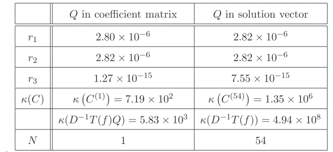
The results are shown in Table 2 and they are similar to the results in Table 1 because better results are obtained when Q is included in the coefficient matrix. It is also seen that

κC(1)

κ(D−1_T(f)Q) =

7.19×102

Q in coefficient matrix Qin solution vector

r1 2.80×10−6 2.82×10−6 r2 2.82×10−6 2.82×10−6 r3 1.27×10−15 7.55×10−15 κ(C) κ C(1)

= 7.19×102 κ C(54)

= 1.35×106

κ(D−1_{T(f)Q) = 5.83×10}3 _κ(D−1_{T(f)) = 4.94×10}8

N 1 54

Table 2

The results of Example 6.2. The first column shows the results when (16) is solved, and the second column shows the results when (34) is solved.

and thus the condition number of the coefficient matrix of the constraint equation in the LSE problem (33) is about one order of magnitude smaller than the condition number of the coefficient matrix of (16). Also, only one iteration is required for the solution of the LSE problem when Q is included in the coefficient matrix, but 54 iterations are required when Qis included in

the solution vector.

7 Discussion

Tables 1 and 2 show that κC(j)_{, the condition number of the coefficient}

matrix of the constraint equation in the LSE problem, is significantly smaller when Q is included in the coefficient matrix than when it is included in the solution vector. This result, which confirms the remarks in Section 2, shows that large combinatorial factors in matrices associated with computations on Bernstein basis polynomials must be considered carefully, such that adverse numerical effects are minimised. Also, fewer iterations are required for the iterative solution of the LSE problem when Q is included in the coefficient matrix. The discussion in this section is therefore restricted to this situation, and the results obtained when Q is included in the solution vector are not considered.

Tables 1 and 2 show that the errors r1 and r2, which are defined in (35) and

(36) respectively, are equal for Example 6.1, and for Example 6.2. It therefore follows that the relative errors in the solutions of the LS and LSE problems are the same, but the advantage of the solution of the LSE problem can be seen from the error r3 in the tables. Since it is approximately equal to 10−16

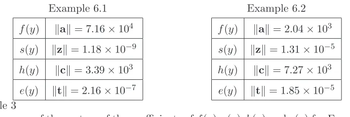
A computed solution is acceptable if its backward error is less than or equal to the error in the given data, and it must therefore be checked that the solutions satisfy this condition. This calculation requires the data in Table 3, which shows the norms of the vectors of the coefficients off(y), h(y), s(y) and e(y), which are defined in (13), (14), (18) and (19) respectively.

Example 6.1

f(y) ka_{k= 7.16×10}4 s(y) kz_{k= 1.18×10}−9 h(y) kc_{k= 3.39×10}3 e(y) kt_{k= 2.16×10}−7

Example 6.2

f(y) ka_{k= 2.04×10}3 s(y) kz_{k= 1.31×10}−5 h(y) kc_{k= 7.27×10}3 e(y) kt_{k= 1.85×10}−5

Table 3

The norms of the vectors of the coefficients off(y), s(y), h(y) ande(y) for Examples 6.1 and 6.2.

It follows from Table 3 that

kzk

kak = 1.65×10

−14 _and ktk

kck = 6.37×10

−11_{, (40)}

for Example 6.1, and

kzk

kak = 6.42×10

−9 _and ktk

kck = 2.54×10

−9_{, (41)}

for Example 6.2, and these normwise errors must be checked against the norm-wise bounds (39) in order to verify that the computed solutions are acceptable. In particular, the random variablesri and rj in (38) are uniformly distributed

in the interval [−1,1], and thus the random variables|ri|and|rj|are uniformly

distributed in the interval [0,1] with mean value 1/2. It therefore follows from (38) that

kδaˆk ≈ ε

2kaˆk and kδˆck ≈ ε

2kˆck. (42)

The normwise backward errors of the solutions also require that the structured perturbations zi and unstructured perturbationsti be considered. In

particu-lar, it follows from (13), (14), (15) and (20) that the corrected forms of the exact polynomials ˆf(y) and ˆh(y) are, respectively,

f(y) +s(y) =

m

X

i=0

(ˆai+δˆai+zi)

m i

!

and

h(y) +e(y) =

m+n

X

i=0

(ˆci+δˆci+ti)

m+n i

!

(1−y)m+n−i_yi_,

and thus the squares of the backward errors of the coefficients of f(y) and h(y) are, respectively,

m

X

i=0

(δˆai+zi)2 =kδaˆk2+kzk2+ 2δaˆTz,

and

m+n

X

i=0

(δcˆi+ti)2 =kδcˆk2+ktk2+ 2δˆcTt.

It follows from (38) that the average values of δˆai and δˆcj are zero, and thus

(42) shows thatη(f) and η(h), the average values of the squares of the back-ward errors of the coefficients off(y) and h(y) satisfy

η(f)2 ≈ ε

2

2

kˆak2+kzk2 and η(h)2 ≈ ε

2

2

kcˆk2+ktk2.

Sinceε= 10−8 _{in Examples 6.1 and 6.2, the errors in the equations kak=kˆak}

and kck=kˆck are negligible, and thus η(f)2 _{and η(h)}2 _{can be approximated}

by

η(f)2 ≈ ε

2

2

kak2+kzk2 and η(h)2 ≈ ε

2

2

kck2+ktk2.

The substitution of (40) and (41) into these approximations yields

η(f)≈ ε

2kak ≈ ε

2kˆak and η(h)≈ ε

2kck ≈ ε 2kcˆk,

for Example 6.1, and

η(f)≈εkak ≈εkˆak and η(h)≈εkck ≈εkˆck,

The condition numberκC(j)

is not the condition number of thejth iteration in the LSE problem because it does not consider the constraint equation. The inverse of the upper triangular matrix R1(j) is computed in step (3c) of

Algorithm 1, and since

κC(j)=κR(j)=κR(1j)

,

it is desirable to minimiseκC(j)

. This minimisation is achieved by including Q in the coefficient matrix, rather than in the solution vector.

The method used in Algorithm 1 is analysed in [1], where it is shown that it is numerically stable. The sensitivity of the solution of the LSE problem to perturbations in C(j)_,q(j) _{and w}(j−1) _{is also considered in [1], and it is}

shown that the forward error r1 is of the form r1 .εκLSE, where κLSE is the

condition number of the LSE problem. Computational results in [1] show that an approximation to this bound may overestimate the forward error achieved in examples, and that this is due to the use of worst case bounds, which cannot be improved.

8 Summary

This paper has considered the method of STLN for the deconvolution of two Bernstein basis polynomials. This method preserves the Tœplitz structure of the coefficient matrix of the equation that defines the deconvolution of two polynomials, and it therefore returns a polynomial. This solution was compared with the solution of a LS problem, and it was shown that this solution defines a polynomial approximation of a rational function, and not a polynomial. It was shown that the method of STLN yields the LSE problem that is solved iteratively by the QR decomposition.

Improved answers were obtained when the coefficient matrix of the equation that defines the deconvolution operation includes the diagonal matrix Q of combinatorial factors. This improvement manifests itself in the requirement for fewer iterations for the solution of the LSE problem, and a smaller condition number of the coefficient matrix of the constraint equation in the LSE problem.

References

39(1):34–50, 1999.

[2] R. T. Farouki and T. N. T. Goodman. On the optimal stability of the Bernstein basis. Mathematics of Computation, 65(216):1553–1566, 1996.

[3] R. T. Farouki and V. T. Rajan. Algorithms for polynomials in Bernstein form.

Computer Aided Geometric Design, 5:1–26, 1988.

[4] R. Goldman. Pyramid Algorithms: A Dynamic Programming Approach to Curves and Surfaces for Geometric Modeling. Morgan Kaufmann Publishers, Academic Press, San Diego USA, 2002.

[5] G. H. Golub and C. F. Van Loan. Matrix Computations. John Hopkins University Press, Baltimore, USA, 1996.

[6] J. Ben Rosen, H. Park, and J. Glick. Total least norm formulation and solution for structured problems. SIAM J. Mat. Anal. Appl., 17(1):110–128, 1996.

[7] J. Ben Rosen, H. Park, and J. Glick. Structured total least norm for nonlinear problems. SIAM J. Mat. Anal. Appl., 20(1):14–30, 1998.

[8] J. V. Uspensky. Theory of Equations. McGraw-Hill, New York, USA, 1948.

[9] J. R. Winkler and M. Hasan. An improved non-linear method for the computation of a structured low rank approximation of the Sylvester resultant matrix. Journal of Computational and Applied Mathematics, 237(1):253–268, 2013.

[10] J. R. Winkler, M. Hasan, and X. Y. Lao. Two methods for the calculation of the degree of an approximate greatest common divsior of two inexact polynomials.

Calcolo, 49:241–267, 2012.

[11] J. R. Winkler and N. Yang. Methods for the computation of the degree of an approximate greatest common divisor of two inexact Bernstein basis polynomials, 2013. Submitted.