A comparative assessment of variable selection methods in urban water demand forecasting

Article

A Comparative Assessment of Variable Selection

Methods in Urban Water Demand Forecasting

Md Mahmudul Haque1, Ataur Rahman1,*, Dharma Hagare1ID _{and Rezaul Kabir Chowdhury}2

1 _{School of Computing, Engineering and Mathematics, Western Sydney University, Second Avenue,}

Kingswood, NSW 2751, Australia; [email protected] (M.M.H.); [email protected] (D.H.)

2 _{School of Civil Engineering and Surveying, University of Southern Queensland, West St, Toowoomba,} QLD 4350, Australia; [email protected]

* Correspondence: [email protected]; Tel.: +61-2-47360145

Received: 9 January 2018; Accepted: 29 March 2018; Published: 3 April 2018

Abstract:Urban water demand is influenced by a variety of factors such as climate change, population growth, socio-economic conditions and policy issues. These variables are often correlated with each other, which may create a problem in building appropriate water demand forecasting model. Therefore, selection of the appropriate predictor variables is important for accurate prediction of future water demand. In this study, seven variable selection methods in the context of multiple linear regression analysis were examined in selecting the optimal predictor variable set for long-term residential water demand forecasting model development. These methods were (i) stepwise selection, (ii) backward elimination, (iii) forward selection, (iv) best model with residual mean square error criteria, (v) best model with the Akaike information criterion, (vi) best model with Mallow’s Cp

criterion and (vii) principal component analysis (PCA). The results showed that different variable selection methods produced different multiple linear regression models with different sets of predictor variables. Moreover, the selection methods (i)–(vi) showed some irrational relationships between the water demand and the predictor variables due to the presence of a high degree of correlations among the predictor variables, whereas PCA showed promising results in avoiding these irrational behaviours and minimising multicollinearity problems.

Keywords:variable selection; principal component analysis; multiple regression; multicollinearity; long-term water demand forecasting; urban water

1. Introduction

Water demand forecasting is a vital element in urban planning and sustainable development of a city. Many important decisions in regards to water demand management, environmental planning and optimum utilization of water resources depend on accurate water demand forecasting. Future water availability is expected to reduce in many urban cities [1] due to several factors such as population growth, changing climatic conditions, pollution of water, scarcity of untapped water sources and increased frequency of droughts [2,3]. Therefore, it is important to have the accurate future water demand projections to ensure adequate water supply to the cities by adopting various strategies such as capacity expansion of existing water supply systems, building new infrastructure and implementation of water demand management policies. Water demand forecasting can be achieved by developing suitable mathematical water demand models based on the predictor variables that influence water demand.

Urban water demand is influenced by a variety of factors such as demographic (e.g., number of population and number of dwellings), climatic (e.g., rainfall, temperature and evaporation),

socioeconomic (e.g., household income and water price) and strategic (e.g., water use restriction and household water conservation programs) [4–10]. Identification of the most important and relevant variables among these candidate variables is crucial in the development of the water demand forecasting model, as the prediction accuracy of the models depends on the selection of an appropriate set of predictor variables. Moreover, many of these variables are highly correlated with each other, which can create multicollinearity problems during the regression-based model development. The multicollinearity problem may lead to unrealistic and biased prediction.

Multiple linear regression analysis has been used widely in developing water demand models since the 1960s; for example, by Gottlieb [11] to develop water demand models for the state of Kansas in the USA to assess the link between water demand and price; by Conley [12] to develop water demand models as a function of water price and number of rainy days in Southern California; by Howe and Linaweaver [13] to examine the relationship among in-house and sprinkler water uses; by Turnovsky [14] to develop household and industrial water demand models in Massachusetts; and by Hankle [15] to assess the impact of introducing meters on residential water demand. More recently, the multiple linear regression technique has been adopted to develop water demand forecasting models by many researchers [16–18]. As noted by Donkor et al. [19], neural networks and hybrid models are more suitable for short-term water demand forecasting, while regression-based models are more appropriate for long-term forecasting.

To deal with the non-linearity in the water demand and predictor variables’ data, logarithmic transformation of these variables is widely adopted in multiple linear regression modelling [19,20]. Artificial intelligence-based methods such as artificial neural network (ANN) [7], fuzzy- and neuro-fuzzy-based methods [21] and support vector regression [22,23] can also be used to deal with the non-linearity; however, these methods are more appropriate for short-term forecasting (e.g., daily or weekly water demand).

The main objective of a variable selection procedure is to identify the correct predictor variables, which have an important influence on the response variable and could provide robust model prediction. A number of different variable selection methods such as stepwise selection, backward elimination, forward selection and principal component analysis (PCA) and different selection criteria have been adopted in the literature to find the optimal set of predictor variables in the model [24–29]. However, Raffalovich et al. [30] and Murtaugh [31] mentioned that no general superior variable selection method exists; some methods are more applicable under certain circumstances, depending on the nature of the problem at hand and the availability of the information. There are several studies on variable selection methods in different fields, for example in ecology [31], in flood estimation [32] and on load forecasting [33]. However, a limited number of studies exist in the literature on variable selection methods in water demand forecasting when multicollinearity is present. A recent study [23] on correlation analysis of variables in modelling short-term water demand has also stressed the need for appropriate variable selection methods for both short-term and long-term water demand modelling in the presence of multicollinearity.

variable set in the development of the long-term water demand forecasting model. Data from the Blue Mountains Water Supply System in the New South Wales, Australia, are used.

The methods compared include: (i) stepwise selection; (ii) forward selection; (iii) backward elimination; (iv) best model with the criteria of residual mean square error; (v) best model with Mallow’sCpcriterion; (vi) best model with the Akaike information criterion (AIC); and (vii) the model

with selected variables based on preprocessing by PCA. The performance of various models is assessed for an independent validation period. This is one of the comprehensive studies in comparing the performance of variable selection methods in long-term water demand forecasting. Moreover, this is one of the few papers that has discussed the multicollinearity problem in water demand forecasting and has highlighted how to resolve the problem. Results of the study are expected to provide important insights into the variable selection methods in water demand modelling to produce more accurate water demand projections. The findings of this study would be useful in enhancing the sustainability of urban water resources and water supply systems in a given region by providing a better tool to estimate future water demand.

2. Study Area and Data

The Blue Mountains region in New South Wales, Australia, has been adopted as the study area, which has a latitude of 33.7◦S and a longitude of 150.3◦ E. Blue Mountains Water Supply System (BMWSS) supplies water to a population of about 48,000 from Faulconbridge to Mount Victoria (Figure1) in the Blue Mountains region, Australia.

As Mount Victoria is over 1000 m above sea level, the temperature is normally 7◦C lower than the coastal Sydney. The average temperature in the Upper Blue Mountains area is around 5◦C and 18◦C in winter (June–August) and summer months (December–February), respectively. The Upper Blue Mountains area has an annual average rainfall of 1050 mm [36].

A large number of water demand variables was adopted in this study: monthly total rainfall (mm), number of rainy days in a month, monthly mean maximum temperature (◦C), monthly average temperature (◦C), monthly total evaporation (mm), monthly solar exposure (MJ/m2), water price (AUS $/Kilolitre(KL)), conservation program participation (CPP) and three water restriction levels (i.e., Levels 1, 2 and 3) imposed in the study area during previous drought periods (2003–2009).

Metered water consumptions in a monthly step and the number of dwellings data for the period of 2003–2011 in the Blue Mountains regions were obtained from Sydney Water. The monthly water consumption values were divided by the number of dwellings to get the ‘per dwelling monthly water consumption (PDMWC)’, which was taken as the response/dependent variable in the analysis. Water price and CPP data were also obtained from Sydney Water. The number of dwellings that were participating in the water demand management programs (e.g., installation of showerheads, flow restrictors, rainwater tanks, water-efficient washing machines and toilets) was referred to as CPP in this study.

The New South Wales Government enforced three levels of water restriction during the millennium drought periods (2003–2009) to manage the limited water supply. Levels 1 and 3 were the most liberal (i.e., minimum restriction on water use) and the most severe level (i.e., high restriction on water use) of restrictions, respectively. These restrictions were mainly imposed on outdoor water use such as garden watering and car washing. The detailed description of the restriction levels and scopes of the levels can be found in Haque et al. [38]. Level 1, 2 and 3 water restrictions were applied to three separate periods during 2003–2009 in the Sydney region based on the severity level of the drought conditions. In this study, these three levels of water restriction were represented by dummy variables (Level 1 dummy variable, Level 2 dummy variable and Level 3 dummy variable); the value of the dummy variables was considered as one when it was in place, otherwise its value was considered to be zero in the data matrices. Meteorological data such as total monthly rainfall, number of rainy days in a month, monthly mean maximum temperature, monthly average temperature, evaporation and solar exposure were obtained from the Sydney Catchment Authority.

3. Methods

In this study, seven variable selection methods were adopted to identify the influential predictor variables in the Blue Mountains Water Supply System for modelling long-term residential water demand. The prediction ability of these methods was evaluated using a split-sample validation technique [39]. The total data period (March 2003–September 2011) was divided into two subsets: (i) March 2003–December 2009 to develop the multiple linear regression (MLR) models and (ii) January 2010–September 2011 to validate the developed models. Sydney Water [40] and Abrams et al. [8] found that despite the existence of no mandatory water restrictions in Sydney, water uses did not increase significantly, i.e., it was increased by only 2–3% during the post restriction periods (2009–2011). It seems that people are preserving their water efficiency behaviours to some degree established during the drought periods. Therefore, during the forecasting of the water demand values for the period of January 2010–September 2011 in the Blue Mountains regions, water use patterns were assumed to be the same as the period of restriction (i.e., the coefficient of Level 3 dummy variables was considered for these periods).

The MLR technique develops a model by establishing a linear relationship between two or more independent variables with a dependent variable. The MLR equation can be expressed as below:

Y=a0+a1x1+a2x2+. . .+aixi+ε (1)

whereYis the dependent variable,a0. . .aiare the coefficients generally estimated by the least squares

develop the MLR models by the seven variable selection methods as the semi-log model was found to perform better in modelling water demand in the BMWSS as noted by Haque et al. [38]. In the semi-log multiple linear regression models in this paper, the dependent variable was taken in the logarithmic form, and the independent variables were incorporated into the model as it lacks any log transformation. The brief descriptions of the seven variable selection methods are given in the following sections.

3.1. Forward Selection

The forward selection method starts with no predictor variables in the model. Then, variables are added, if needed, in the model one by one, and the forward selection method calculates thep-value (i.e., significance) for each of the variables. If the calculatedp-value for the variable is found to be less than the critical value, then the forward selection method keeps the variable in the model, otherwise the variable is removed from the model. This is done iteratively until all the variables in the model have ap-value less than 0.1. In this study, a partial F criterion [31] was used to add or delete variables in the multiple linear regression models. The partial F statistic was calculated by Equation (2) and compared with an F distribution to estimate thep-value. A critical thresholdp-value of 0.1 was adopted in this study.

Fi =

(SSEi−1−SSEi) SSEi

×n−k−1

k (2)

whereSSEi−1andSSEi are the sum of square errors before and after the exclusion of a predictor

variable,nis the number of data points andkis the number of predictor variables.

3.2. Backward Elimination

The backward elimination method starts with all the predictor variables in the model and removes one variable at a time using ap-value. In the first step, thep-value is calculated for all the predictor variables, and the variable with the largestp-value that exceeds the criticalp-value is deleted. In the second step, thep-value is calculated for the remaining variables, and again, the variable with the highestp-value that exceeds the criticalp-value is deleted. The process is iterated until the highest p-value of a variable is less than the criticalp-value, indicating that the corresponding variable is not redundant in the presence of the other variables in the model.

3.3. Stepwise Selection

The stepwise selection method combines certain aspects of forward selection and backward elimination methods. Like the forward selection method, it starts with no variable in the model, and variables are added one by one to the model by fulfilling thepcriteria (p< 0.1). After a variable is added in the model, the stepwise selection method examines all the variables in the model and deletes any variable that show ap-value greater than the critical value. The next variable is added in the model only after checking the model and deleting any variables if necessary. This process continues till none of the variables outside the model have ap-value less than the critical value and every single variable in the model satisfies thepcriteria.

3.4. Best Model with Residual Mean Square Error Criteria

If there arekpotential predictor variables, then the possible number of prediction models would be 2k. The number of independent variables considered in this study was 11. In the best model with MSE criteria, all the possible models (211) were evaluated, and the model with the lowest value of MSE was selected. The MSE measures the variance for each of the models and is calculated by the following equation:

MSE= ∑ Y−Yp 2

whereYandYpare the observed and predicted water demand value, respectively,nis the number of

data points andkis the number of independent variables.

3.5. Best Model with the Akaike Information Criterion

The AIC procedure was proposed by Akaike [42], and it selects the model with the minimum value of the AIC, which can be calculated by the following equation:

AIC=nlog(MSE) +2k (4)

3.6. Best Model with Mallow’s CpCriterion

TheCpcriterion was proposed by Mallow [43] for univariate regression analysis, and it selects

the model with the minimum value of theCp statistic. The Cp statistic can be calculated by the

following equation:

Cp= SSEk

S2 −(n−2k) (5)

whereS2is the MSE for the full model (i.e., when all the predictor variables are included in the model) andSSEk is the residual sum of squares for the subset model that containsknumber of predictor

variables in the model.

3.7. Principal Component Analysis

Principal component analysis transforms a data-set of original variables into a new a dataset of uncorrelated derived variables. These new derived variables are called principal components (PCs), which are the results of linear functions of the original variables. During the PCA analysis, sums of the variances are equal for both the original and derived variables. The highest amount of variance in the data is explained by the first PC, and then, the second PC explains the next highest variance, and so on, for all the remaining PCs. The value of PC 1 and PC 2 can be obtained by Equations (6) and (7). The remaining PCs can be obtained in the same way. In PCA analysis, the first few PCs generally explain most of the variance in the data matrices that can be used to characterize the original observations [44,45]. The dimensionality of the original dataset can be reduced by considering the first few PCs in the PCA analysis. More details on the PCA method can be found in Haque et al. [29].

PC1=a11x1+a12x2+. . .+a1kxk= k

∑

j=1

a1jxj (6)

PC1=a21x1+a22x2+. . .+a2kxk= k

∑

j=1

a2jxj (7)

wherex1,x2,...,xkrepresent the original variables in the data matrix andaijrepresent the eigenvectors.

4. Results

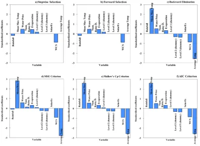
statistically insignificant in stepwise regression analysis. Water price and Level 1 dummy variables were found to have positive coefficients, which indicates that the water demand will increase with the increase of these two variables. However, this relationship is irrational as water demand would go down with an increase of water price and restriction levels. Variables in the forward selection regression models were found to be the same as the stepwise regression model.

Figure 2.Standardized coefficients of the independent variables for each variable selection method.

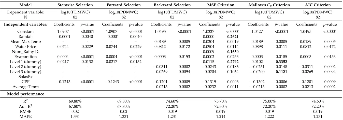
Table 1.Modelling results from the developed models adopting different variable selection methods. CPP, conservation program participation.

Model Stepwise Selection Forward Selection Backward Selection MSE Criterion Mallow’sCpCriterion AIC Criterion

Dependent variable: log10(PDMWC) log10(PDMWC) log10(PDMWC) log10(PDMWC) log10(PDMWC) log10(PDMWC)

N 82 82 82 82 82 82

Independent variables: Coefficients p-value Coefficients p-value Coefficients p-value Coefficients p-value Coefficients p-value Coefficients p-value

Constant 1.0907 <0.0001 1.0907 <0.0001 1.0495 <0.0001 1.0327 <0.0001 1.0427 <0.0001 1.0495 <0.0001

Rainfall −0.0001 0.0040 −0.0001 0.0040 - - 0.0000 0.2621 - - -

-Mean Max Temp - - - - 0.0189 0.0005 0.0204 0.0019 0.0189 0.0005 0.0189 0.0005

Water Price 0.0744 0.0229 0.0744 0.0229 0.0812 0.0172 0.0904 0.0114 0.0898 0.0111 0.0812 0.0172

Num_Rainy D. - - - 0.0009 0.1650 - - -

-Evaporation 0.0004 <0.0001 0.0004 <0.0001 0.0003 0.0153 0.0002 0.0253 0.0003 0.0185 0.0003 0.0153

Level 1 (dummy) 0.0217 0.0132 0.0217 0.0132 - - 0.0115 0.2792 0.0102 0.3352 -

-Level 2 (dummy) - - - - −0.0311 0.0002 −0.0243 0.0186 −0.0251 0.0148 −0.0311 0.0002

Level 3 (dummy) - - - - −0.0269 0.0094 −0.0204 0.1064 −0.0200 0.1121 −0.0269 0.0094

SolasEx - - -

-CPP −0.1243 <0.0001 −0.1243 <0.0001 −0.1201 0.0009 −0.1319 0.0006 −0.1302 0.0006 −0.1201 0.0009

Average Temp - - - - −0.0213 0.0002 −0.0232 0.0011 −0.0213 0.0002 −0.0213 0.0002

Model performance

R2 _{69.80% 69.80% 74.60% 75.70% 75.00% 74.60%}

Adj. R2 67.80% 67.80% 72.20% 72.30% 72.20% 72.20%

RMSE 0.02 0.02 0.019 0.019 0.019 0.019

MAPE 1.331 1.331 1.231 1.214 1.222 1.231

In the best model with Mallow’sCpcriterion, eight predictor variables out of 11 were found to

be statistically significant. Rainfall, number of rainy days and solar exposure showed no effect on water demand. This model also showed some irrational relationship like earlier models as water price and Level 1 dummy variables showed positive correlation with water demand, and average temperature showed negative correlation. In the best model with the AIC criterion, seven variables out of 11 were found to be statistically significant. Rainfall, number of rainy days, Level 1 dummy and solar exposure showed no relation with water demand. This model also had some irrational characteristics like earlier models. It can be seen in Figure2and Table1that all of the selection methods considered different sets of variables to be taken as final input in their regression models. Moreover, all of them had some irrational relationships with the water demand. The more likely reason for these irrational relationships is the presence of multicollinearities among the independent variables. In terms of modelling results’ statistics as shown in Table1, the best model with the MSE criterion was found the best among those six models as it had the highest R2and Adjusted(Adj.) R2 values and the lowest RMSE (root mean square error) and MAPE (mean absolute percentage error) values. However, the models from 3–6 ((iii) backward elimination; (iv) best model with the criteria of residual mean square error; (v) best model with Mallow’sCpcriterion; (vi) best model with the Akaike

information criterion (AIC)) all had comparable results with each other.

Table2presents the Pearson correlation matrices of the water demand variables, which can be used to identify the existence of the multicollinearities between the independent variables and the strong and weak relationship between them. Notable correlation coefficients between the variables are highlighted in bold. The maximum correlation coefficient was found to be 0.99, which was between monthly mean maximum temperature and monthly average temperature. The second maximum correlation coefficient was found between CPP and water price, which was 0.95. Evaporation, mean maximum temperature and average temperature were found to be highly correlated with solar exposure. Rainfall and number of rainy days were also found to be highly correlated with each other. These high correlations among the independent variables indicate the presence of a strong multicollinearity, which is more likely to produce biased results or unrealistic relationships in the regression analysis.

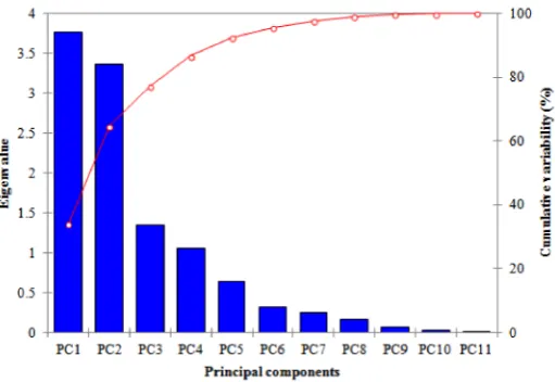
The results of PCA on the 11 independent variables to explain water consumption level are presented in Figure3and Table3. Eigen values of each PC’s and cumulative variance explained by the PC’s are presented in Figure3, where it can be seen that the first four PC’s explained around 85% of the variability and had eigenvalues greater than one. Therefore, in this study, PC 1–PC 4 were chosen to find the important variables to estimate water demand. The ‘bold marked loads’ in Table3represent a high correlation between the variables and corresponding PC.

Table 2.Pearson correlation matrix of the independent variables.

Variables Rainfall Num_Rainy D. Mean Max_Temp Average_Temp Evaporation SolarEx Water Price CPP _(Dummy)Level 1 _(Dummy)Level 2 _(Dummy)Level 3

Rainfall 1.00 0.68 0.21 0.27 0.01 0.10 0.14 0.13 −0.05 −0.01 0.11

Num_Rainy D. 1.00 0.26 0.32 0.02 0.20 0.26 0.25 −0.12 −0.12 0.23

Mean Max Temp 1.00 0.99 0.79 0.86 0.07 0.07 0.19 0.00 0.02

Average Temp 1.00 0.75 0.82 0.08 0.07 0.19 −0.01 0.02

Evaporation 1.00 0.86 −0.12 −0.14 0.37 0.07 −0.25

SolarEx 1.00 0.19 0.22 0.10 0.00 0.08

Water Price 1.00 0.95 −0.34 −0.37 0.70

CPP 1.00 −0.37 −0.38 0.80

Level 1 (dummy) 1.00 −0.14 −0.47

Level 2 (dummy) 1.00 −0.59

Level 3 (dummy) 1.00

It can be seen in Table3that rainfall had greater variable loading in PC 3 than in the number of rainy days. Therefore, rainfall was chosen to be in the regression model, and the number of rainy days was discarded to avoid the multicollinearity problem. After removing the highly correlated variables, rainfall, mean maximum temperature, CPP, water price, Level 1, Level 2 and Level 3 dummy variables were considered in the regression analysis. To select the best variable between water price and CPP, three separate models were developed with the dataset of3 March–9 December and compared with each other in estimating water demand for the independent data period (10 January–11 September).

• Model 1: Rainfall, mean maximum temperature, CPP, Level 1, Level 2, Level 3

• Model 2: Rainfall, mean maximum temperature, water price, Level 1, Level 2, Level 3

• Model 3: Rainfall, mean maximum temperature, CPP, water price, Level 1, Level 2, Level 3

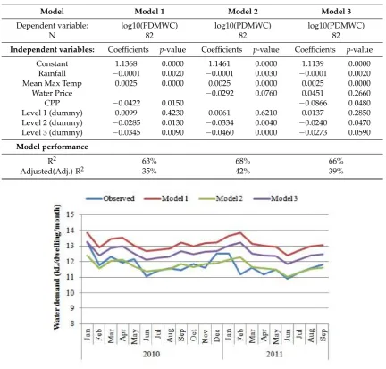
During the development of the regression model for the above three conditions, the Level 1 dummy variable was found to be statistically insignificant for all of the cases as thep-value of the regression coefficient was found to be more than 0.4 (Table4). Therefore, the Level 1 dummy variable was discarded from the above three models. Simulation results of Models 1, 2 and 3 for the independent data period are presented in Figure4. It can be seen that the model with water price (Model 2) produced better simulation results than the other two models. Even Model 3 (with water price and CPP together) was found to produce poorer results than Model 1 and Model 2 due to the effect of the multicollinearity problem of the variables. These results indicate that inclusion of many variables in the model does not necessarily increase the model efficiency. In addition, Model 2 did not show any counter-intuitive relation with the temperature and water price variables, as can be seen in Table4.

Table 3.Variable loadings (correlations between original variables and the first four PCs).

Variables PC 1 PC 2 PC 3 PC 4

Rainfall 0.35 0.33 0.75 0.24

Num_Rainy D. 0.34 0.53 0.62 0.21

Mean Max Temp 0.97 −0.01 −0.07 −0.08

Average Temp 0.96 0.03 −0.01 −0.04

Evaporation 0.88 −0.27 −0.22 −0.04

SolarEx 0.92 0.08 −0.18 −0.18

Water Price 0.00 0.86 −0.13 −0.07

CPP 0.02 0.92 −0.18 −0.10

Level 1 (dummy) 0.24 −0.49 −0.18 0.71

Level 2 (dummy) 0.01 −0.54 0.42 −0.62

Level 3 (dummy) −0.05 0.88 −0.23 −0.03

Table 4.Modelling results by the developed models adopting PCA analysis.

Model Model 1 Model 2 Model 3

Dependent variable: log10(PDMWC) log10(PDMWC) log10(PDMWC)

N 82 82 82

Independent variables: Coefficients p-value Coefficients p-value Coefficients p-value

Constant 1.1368 0.0000 1.1461 0.0000 1.1139 0.0000

Rainfall −0.0001 0.0020 −0.0001 0.0030 −0.0001 0.0020 Mean Max Temp 0.0025 0.0000 0.0025 0.0000 0.0025 0.0000

Water Price −0.0292 0.0760 0.0451 0.2660

CPP −0.0422 0.0150 −0.0866 0.0480

Level 1 (dummy) 0.0099 0.4230 0.0061 0.6210 0.0137 0.2850 Level 2 (dummy) −0.0285 0.0130 −0.0334 0.0040 −0.0240 0.0470 Level 3 (dummy) −0.0345 0.0090 −0.0460 0.0000 −0.0273 0.0590

Model performance

R2 63% 68% 66%

Adjusted(Adj.) R2 35% 42% 39%

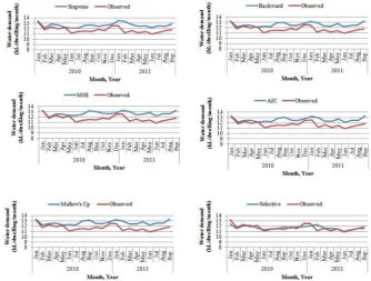
Finally, the important predictor variables for estimating water demand in the BMWSS were found to be monthly total rainfall, monthly mean maximum temperature, water price and Level 2 and Level 3 water restrictions. The comparison of the forecasted results by all the developed models (i.e., stepwise, forward, backward, MSE, Mallow’sCp, AIC and selection of variables after PCA (i.e., Model 2)) for

the independent data period is presented in Figure5, which also shows that the regression model with the selected independent variables performed better than all the other models. These results indicate that the selected independent variables are capable of simulating monthly water demand with a higher accuracy, and the developed model is largely free from the multicollinearity problem. This also indicates that PCA performed better in selecting the independent variables than the other methods adopted in this study, which has the potential to produce forecasting results with better accuracy. This method is easy to implement and can be used in other water supply systems around the world to identify the influential water demand variables and estimate water demand.

Figure 5. Comparison of modelled results of all the developed models (i.e., stepwise, forward, backward, MSE, Mallow’sCp, AIC and selective variable regression (Model 2)).

5. Conclusions

Seven variable selection methods in the context of linear regression (i.e., stepwise selection, forward selection, backward elimination, MSE criterion, Mallow’sCp criterion, AIC criterion and

presence of high degree of multicollinearities among the predictor variables. The findings of this paper are directly applicable to the study area in Australia; however, the developed technique can be adapted to other countries having different water use and climatic characteristics to develop water demand forecasting models.

Acknowledgments:The authors express their sincere thanks to Pei Tillman and Frank Spaninks of Sydney Water for their assistance in collating and providing the data. Further, the authors are grateful to Lucinda Maunsell and Peter Cox of Sydney Water, as well as Mahes Maheswaran and Golam Kibria of WaterNSW for their cooperation and assistance during data collection and analysis.

Author Contributions:Md Mahmudul Haque and Ataur Rahman conceived of and designed the research route. Md Mahmudul Haque collected and analysed the data. Md Mahmudul Haque and Ataur Rahman wrote the paper. Dharma Hagare and Rezaul Kabir Chowdhury reviewed the technical contents and edited the paper.

Conflicts of Interest:The authors declare no conflict of interest.

References

1. Notter, B.; MacMillan, L.; Viviroli, D.; Weingartner, R.; Liniger, H.P. Impacts of environmental change on water resources in the Mt.Kenya region. J. Hydrol.2007,343, 266–278.

2. Koutroulis, A.G.; Tsanis, I.K.; Daliakopoulos, I.N.; Jacob, D. Impact of climate change on water resources status: A case study for Crete Island, Greece.J. Hydrol.2013,479, 146–158. [CrossRef]

3. Makki, A.A.; Stewart, R.A.; Beal, C.D.; Panuwatwanich, K. Novel bottom-up urban water demand forecasting model: Revealing the determinants, drivers and predictors of residential indoor end-use consumption.

Resour. Conserv. Recycl.2015,95, 15–37. [CrossRef]

4. Gato, S.; Jayasuriya, N.; Roberts, P. Temperature and rainfall thresholds for base use urban water demand modelling.J. Hydrol.2007,337, 364–376. [CrossRef]

5. Arbués, F.; Villanúa, I.; Barberán, R. Household size and residential water demand: An empirical approach.

Aust. J. Agric. Resour. Econ.2010,54, 61–80. [CrossRef]

6. House-Peters, L.; Pratt, B.; Chang, H. Effects of urban spatial structure, sociodemographics, and climate on residential water consumption in Hillsboro, Oregon.J. Am. Water Resour. Assoc.2010,46, 461–472. [CrossRef] 7. Babel, M.S.; Shinde, V.R. Identifying prominent explanatory variables for water demand prediction using artificial neural networks: A case study of Bangkok.Water Resour. Manag.2011,25, 1653–1676. [CrossRef] 8. Abrams, B.; Kumaradevan, S.; Sarafidis, V.; Spaninks, F. An econometric assessment of pricing Sydney’s

residential water use.Econ. Rec.2012,88, 89–105. [CrossRef]

9. Haque, M.M.; Rahman, A.; Hagare, D.; Kibria, G. Probabilistic water demand forecasting using projected climatic data for Blue Mountains water supply system in Australia.Water Resour. Manag.2014,28, 1959–1971. [CrossRef]

10. Felfelani, F.; Kerachian, R. Municipal water demand forecasting under peculiar fluctuation in population: A case study of Mashhad touristy city.Hydrol. Sci. J.2015,61, 1524–1534. [CrossRef]

11. Gottlieb, M. Urban domestic demand for water: A Kansas case study.Land Econ.1963,39, 204–210. [CrossRef] 12. Conley, B.C. Price elasticity of the demand for water in Southern California.Ann Reg. Sci.1967,1, 180–189.

[CrossRef]

13. Howe, C.W.; Linaweaver, F.P. The impact of price on residential water demand and its relation to system design and price structure.Water Resour. Res.1967,3, 13–32. [CrossRef]

14. Turnovsky, S.J. The demand for water: Some empirical evidence on consumers’ response to a commodity uncertain in supply.Water Resour. Res.1969,5, 350–361. [CrossRef]

15. Hanke, S.H. Demand for water under dynamic conditions.Water Resour. Res.1970,6, 1253–1261. [CrossRef] 16. Polebitski, A.S.; Palmer, R.N. Seasonal residential water demand forecasting for census tracts.J. Water Resour.

Plan. Manag.2009,136, 27–36. [CrossRef]

17. Wei, S.; Lei, A.; Islam, S.N. Modeling and simulation of industrial water demand of Beijing municipality in China.Front. Environ. Sci. Eng. China2010,4, 91–101. [CrossRef]

19. Donkor, E.A.; Mazzuchi, T.A.; Soyer, R.; Alan Roberson, J. Urban water demand forecasting: Review of methods and models.J. Water Resour. Plan. Manag.2014,140, 146–159. [CrossRef]

20. Billings, R.B.; Jones, C.V.Forecasting Urban Water Demand; American Water Works Association: Denver, CO, USA, 2011.

21. Tabesh, M.; Dini, M. Fuzzy and neuro-fuzzy models for short-term water demand forecasting in Tehran.

Iran. J. Sci. Technol.2009,33, 61–77.

22. Bai, Y.; Wang, P.; Li, C.; Xie, J.; Wang, Y. A multi-scale relevance vector regression approach for daily urban water demand forecasting.J. Hydrol.2014,517, 236–245. [CrossRef]

23. Brentan, B.M.; Luvizotto E., Jr.; Herrera, M.; Izquierdo, J.; Pérez-García, R. Hybrid regression model for near real-time urban water demand forecasting.J. Comput. Appl. Math.2017,309, 532–541. [CrossRef]

24. Barrett, B.E.; Gray, J.B. A computational framework for variable selection in multivariate regression.

Stat. Comput.1994,4, 203–212. [CrossRef]

25. McQuarrie, A.D.; Tsai, C.Regression and Time Series Model Selection; World Scientific Publishing Co., Pte. Ltd.: Singapore, 1998.

26. Sauerbrei, W.; Royston, P.; Binder, H. Selection of important variables and determination of functional form for continuous predictors in multivariable model building. Stat. Med. 2007,26, 5512–5528. [CrossRef] [PubMed]

27. Lee, H.; Ghosh, S.K. Performance of information criteria for spatial models.J. Stat. Comput. Simul.2009,79, 93–106. [CrossRef] [PubMed]

28. Sharma, M.J.; Yu, S.J. Stepwise regression data envelopment analysis for variable reduction.

Appl. Math. Comput.2015,253, 126–134. [CrossRef]

29. Haque, M.M.; Egodawatta, P.; Rahman, A.; Goonetilleke, A. Assessing the significance of climate and community factors on urban water demand.Int. J. Sustain. Built Environ.2015,4, 222–230. [CrossRef] 30. Raffalovich, L.E.; Deane, G.D.; Armstrong, D.; Tsao, H.S. Model selection procedures in social research:

Monte-Carlo simulation results.J. Appl. Stat.2008,35, 1093–1114. [CrossRef]

31. Murtaugh, P.A. Performance of several variable selection methods applied to real ecological data.Ecol. Lett.

2009,12, 1061–1068. [CrossRef] [PubMed]

32. Haddad, K.; Rahman, A. Regional flood frequency analysis in eastern Australia: Bayesian GLS regression-based methods within fixed region and ROI framework—Quantile Regression vs. Parameter Regression Technique.J. Hydrol.2012,430–431, 142–161. [CrossRef]

33. Xie, J.; Hong, T. Variable selection methods for probabilistic load forecasting: Empirical evidence from seven States of the United States.IEEE Trans. Smart Grid.2017. [CrossRef]

34. Gagliardi, F.; Alvisi, S.; Kapelan, Z.; Franchini, M.A. probabilistic short-term water demand forecasting model based on the Markov Chain.Water2017,9, 507. [CrossRef]

35. Pacchin, E.; Alvisi, S.; Franchini, M.A. short-term water demand forecasting model using a moving window on previously observed data.Water2017,9, 172. [CrossRef]

36. Bluemountainsaustralia.com (n.d.). Location and Maps. Available online:http://www.bluemts.com.au/ info/about/maps/(accessed on 12 December 2017).

37. Bluemountainsaustralia.com (n.d.). Climate. Available online:http://www.bluemts.com.au/info/about/ climate/(accessed on 12 December 2017).

38. Haque, M.M.; Hagare, D.; Rahman, A.; Kibria, G. Quantification of water savings due to drought restrictions in water demand forecasting models.J. Water Resour. Plan. Manag.2014,140, 04014035. [CrossRef]

39. Browne, M.W. Cross-validation methods.J. Math. Psychol.2000,44, 108–132. [CrossRef] [PubMed]

40. Sydney Water.Water Conservation and Recycling Implementation Report, 2009–2010; Sydney Water Corporation: Sydney, NSW, Australia, 2010.

41. Montgomery, D.C.; Peck, E.A.; Vining, G.G.Introduction to Linear Regression Analysis; John Wiley and Sons: New York, NY, USA, 2011.

42. Akaike, H. A new look at the statistical model identification.IEEE Trans. Autom. Control1974,19, 716–723. [CrossRef]

44. Abdul-Wahab, S.A.; Bakheit, C.S.; Al-Alawi, S.M. Principal component and multiple regression analysis in modelling of ground-level ozone and factors affecting its concentrations.Environ. Model. Softw.2005,20, 1263–1271. [CrossRef]

45. Olsen, R.L.; Chappell, R.W.; Loftis, J.C. Water quality sample collection, data treatment and results presentation for principal components analysis-literature review and Illinois River watershed case study.

Water Res.2012,46, 3110–3122. [CrossRef] [PubMed]