This is a repository copy of
Study of drag and orientation of regular particles using stereo
vision, Schlieren photography and digital image processing
.
White Rose Research Online URL for this paper:
http://eprints.whiterose.ac.uk/112451/
Version: Accepted Version
Article:
Carranza, F. and Zhang, Y. orcid.org/0000-0002-9736-5043 (2017) Study of drag and
orientation of regular particles using stereo vision, Schlieren photography and digital image
processing. Powder Technology, 311. pp. 185-199. ISSN 0032-5910
https://doi.org/10.1016/j.powtec.2017.01.010
[email protected] https://eprints.whiterose.ac.uk/ Reuse
This article is distributed under the terms of the Creative Commons Attribution-NonCommercial-NoDerivs (CC BY-NC-ND) licence. This licence only allows you to download this work and share it with others as long as you credit the authors, but you can’t change the article in any way or use it commercially. More
information and the full terms of the licence here: https://creativecommons.org/licenses/ Takedown
If you consider content in White Rose Research Online to be in breach of UK law, please notify us by
1
Study of drag and orientation of regular particles using stereo vision,
Schlieren photography and digital image processing
F. Carranza, Y. Zhang*
Department of Mechanical Engineering, University of Sheffield, Mappin Street, Sheffield, S1 3JD, UK
Abstract
A new experimental, image-based methodology suitable to track the changes in orientation of non-spherical particles and their influence on the drag coefficient as they settle in fluids is presented. Given the fact that non-spherical solids naturally develop variations in their angular orientation during the fall, none-intrusiveness of the technique of analysis is of paramount importance in order to preserve the particle/fluid interaction undisturbed. Three-dimensional quantitative data about the motion parameters is obtained through single-camera stereo vision whilst qualitative visualizations of the adjacent fluid patterns are achieved with Schlieren photography. The methodology was validated by comparing the magnitudes of the drag coefficient of a set of spherical particles at terminal velocity conditions against those estimated from drag correlations published in the literature. A noteworthy similarity was attained. During the fall of non-spherical solids, once the particle Reynolds number approximated 163 for disks, and 240 for cylinders, or exceeded those values, secondary motions composed by regular oscillations and tumbling were present. They altered the angular orientation of the particles with respect to the main motion direction and caused complete turbulent patterns in the surrounding flow, therefore affecting the instantaneous projected area, drag force, and coefficient of resistance. The impact of the changes in angular orientation onto the drag coefficient was shown graphically as a means for reinforcing existing numerical approaches, however, an explicit relation between both variables could not be observed.
Keywords: stereo vision, Schlieren photography, terminal velocity, drag coefficient, angle of incidence
1. Introduction
The motion of particles in fluids appears in many industrial applications, such as pneumatic conveyors, and pulverized-fuel boilers for instance. Furthermore, in the design and modelling of such installations the size, shape, and aerodynamics of the solids involved are of paramount importance since they have a direct effect on the patterns of flow, heat transfer rates, and combustion processes, affecting the overall performance of the installations in consequence. Although the industrial devices deal with a large number of particles, understanding the motion of a single one is critical since it provides the basis to model multi-particle systems. Moreover, quantities typical from studies of settling solids, such as the terminal velocity UT and drag coefficient CD, are essential for the design equations. Nevertheless, further research in this field is still needed, mainly when the shape of the particles involved is not spherical.
As it can be observed from the correlations listed in Table 1, the drag coefficient of a spherical object can be expressed solely in terms of the particle Reynolds number ReP,
2 however, as seen in Table 2, for a non-spherical particle extra parameters representing the shape need to be included. Nonetheless, the angular orientation of the solid with respect to the direction of motion is normally omitted, despite the fact that not only it does alter the magnitude of the instantaneous projected area AP, but also changes the pattern of the surrounding flow significantly, especially at high ReP.
In this research, for a non-spherical object, the particle Reynolds number is based on the diameter of the same volume equivalent sphere dsph; therefore, if UT is obtained directly from the experimental analysis and ρf and μ are the fluid density and dynamic viscosity, respectively, ReP can be computed as follows
= (9)
In this paper UT is determined experimentally, however for the purpose of comparison, the analytical procedure advised by Haider and Levenspiel [2] to predict UT for both spherical and non-spherical particles was also used. Being ρP the particle density, the acceleration due to gravity, and ∗ a dimensionless diameter defined as
∗= −
/
(10)
the equation they proposed to calculate UT for spheres is
= 18 ∗ . + 0.321 ∗ . . − / (11)
and for non-spheres, in the interval 0.5 < ∅ < 1, is
= 18
∗ +
2.3348 − 1.7439∅
∗ . −
/
(12)
In Equations (5), (6), (7), and (11), Ø is known as the sphericity, and it is defined as the ratio between the surface area of the same volume sphere and the actual particle surface area [9]. Additionally, in Equation (7), the lengthwise sphericity ∅∥is obtained through the division of the projected area of the same volume sphere by the particle true projected area, and the crosswise sphericity ∅ is calculated from the ratio of the projected area of the same volume sphere and the result of subtracting the average of the longitudinally projected true area to half the true particle surface area [7]. Though ∅∥ and ∅ were developed to consider the influence of the angular variation of the solid, their accurate calculation is substantially complicated. The aspect ratio σ is computed dividing the largest particle dimension by the smallest one.
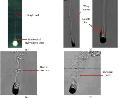
3 turn changes in function of ReP, as illustrated in Figure 1. Magarvey and Bishop [10, 11] have reported that a stable, symmetrical fluid circulation zone behind a free-falling sphere prevails up to ReP ~ 210 (Figure 1a). Afterwards, asymmetry appears, occupying the whole wake region at ReP ~ 290, and giving chance to vortex shedding, which, initially, can be highly regular in the form of the so-called hairpin structures (Figure 1b), nevertheless, regularity diminishes as ReP increases, and at ReP ~ 1000, complete turbulence dominates the wake behind the sphere (Figure 1c). These flow phenomena, also observed by Veldhuis et al., and Veldhuis and Bieshuvel [12,13], have been made responsible for generating deviations in the sphere trajectory.
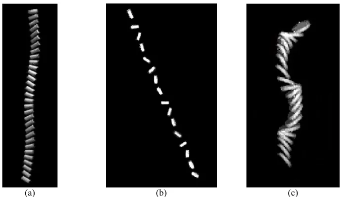
Detailed descriptions of the characteristics of the flow around free settling objects with non-spherical form are scarce in the literature. Nonetheless, it is believed that the evolution from stable, symmetrical configurations at low ReP into complete irregular, turbulent patterns as ReP grows also occurs. Moreover, Marchildon et al. [14] have reported that for a settling cylinder once ReP > 80 regular oscillations may accompany the main motion, yet for ReP > 300 they always appear (Figure 2a). Additionally, Chow and Adams [8] have observed that cylinders which meet the condition (ρPD/ρfL)0.5 > 0.5 so long as ReP > 200 will experience oscillation and those for which (ρPD/ρfL)0.5 > 1.5 will endure tumbling during their settling. The quantities D and L are the diameter and length, respectively.
Stringham et al. [15] have found that the orientation of a disk in free fall changes after certain value of ReP as consequence of alterations in the pressure distribution around the object. They witnessed the presence of oscillation, gliding, and tumbling for ReP > 400. However, these motions can appear at lower values of ReP, as illustrated in Figure 2b for a tumbling disk. Figure 2c shows the case of an oscillating disk. They also argued that the magnitude of the coefficient of resistance is considerably affected by these phenomena. For instance, the experimental values of CD they reported for free-falling disks fluctuated between 5 and 10 for the Reynolds interval 10 < ReP < 1000.
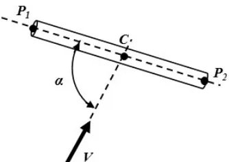
Aiming for a direct approach to involve the angular orientation changes, product of the secondary motions and other instabilities, into the calculation of the coefficient of resistance, in different numerical works it has been recommended to express CD as a function of the angle of incidence, α, which is the angle between the particle longest axis P1P2 and the fluid velocity vector V (Figure 3). Rosendahl [16] has suggested an equation
of the form
= , °+ , °− , ° (13)
where , ° is the drag coefficient at zero angle of incidence and occurs when the particle projected area is minimum. , ° corresponds to the largest angle of incidence, which takes place when the solid exposes its maximum projected area perpendicular to the flow. According to the author both of them should be calculated experimentally. Later, Mandø and Rosendahl [17] advised to replace for only, arguing that a superior accuracy can be accomplished. Zastawny et al. [18] suggested to allow the exponent of in Equation (13) to be variable, therefore the method they proposed is
4 where
, °= ( ) + ( ) (15)
, °= ( ) + ( ) (16)
which is appropriate for particles of ellipsoidal, disk, and cylindrical shape, and valid up to ReP = 300. In order to know the values of the constants a0,…,a8, the reader is referred to the corresponding publication. The main drawback of Equations (13) and (14) is that they are based on the assumption of a stationary particle exposed to a moving fluid, therefore skipping the effects of the secondary motions and wake structures described in the previous paragraphs. In addition, the applicability of Equation (14) is further restricted provided that the secondary motions normally develop after ReP exceeds 220 or even higher values in some cases. Equation (7) is also affected by the same assumption to some extent, given that the authors combined experimental data from the literature with numerical results where the particle was also held static.
Preserving the interaction between the solid and the fluid uninterrupted is critical in order to encompass in the analysis all of the phenomena affecting the orientation and resistance experienced by the particles. For instance, it has been established that the value of CD for a free-falling sphere may be 15 to 30 % higher than that of a stationary sphere [4]. Therefore, in this work the motion of freely settling regular particles was investigated using visual, non-intrusive methods only: stereo vision to obtain three-dimensional (3D) data, and Schlieren photography to observe the structures of the surrounding flow and the trails formed downstream.
The particles studied were spheres, cylinders, and disks. The spheres were employed to expose and validate the methodology of analysis, whilst the other shapes were used to examine the effects of secondary motions on the particle aerodynamics as well as the influence of angular orientation changes on the drag coefficient. In order to obtain time-resolved data, the recording was done exclusively with high-speed cameras. Digital image processing was applied to enhance the particle pictures and extract the information required for the stereo analysis.
2. Material and methods
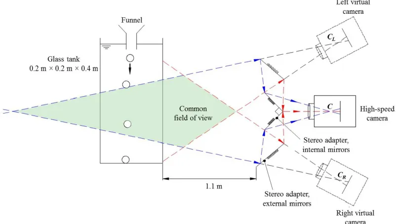
5 An alternative way to generate 3D data is the approach used by Stringham et al. [15], which consists on placing two cameras at right angle with respect to each other, so that the motion of the particles is recorded in two perpendicular planes. Marchildon et al. [14] and Veldhuis et al. [12, 13, 23] also employed a similar configuration but using only one camera and an arrangement of perpendicular mirrors to see the motion on both normal planes. Even though both methods offer a straightforward means to calculate the 3D coordinates of the moving particles, they require a highly accurate alignment of the cameras or mirrors which considerably decreases the flexibility of this alternative approach.
The process of stereo vision can also be accomplished by the use of two or more cameras, as it has been recently suggested by Marcus et al. [24] and Krueger et al. [25]. In this way, the particle motion can be studied within a bigger field of view with larger spatial resolution, however, the more cameras are used the less versatility the stereo system has, the more calibrations need to be done, and the higher the disparity is [26]. Therefore, it is always desirable to work with stereo systems which keep the disparity as low was possible, which is the main advantage of the one-camera arrangements, such as the one employed in this investigation, as long as working with a reduced field of view does not pose any obstacle to the researched phenomena.
Spheres, cylinders, and disks of different sizes and materials, as well as water, glycerin, and water/glycerin mixtures were used to generate the following particle Reynolds number interval: 0.1 < ReP < 5000. The dimensions and materials of the solids are provided in Table 3, whilst in Table 4 the matrix of experiments and the fluid properties are listed. The drop of each particle was repeated between 3 to 5 times to ensure consistency in the results. Because the glycerin and glycerin/water mixtures did not allow Schlieren visualization, this one was implemented only for the cases where the solids sank in pure water (mixture 0/100 in Table 4).
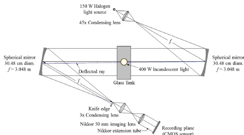
The setup of the Z-type Schlieren configuration used to visualize the structures of the flow adjacent to the particles is displayed in Figure 5. In order to generate the conditions required for Schlieren photography in water, Fiedler et al. [27] recommended to create gradients in the temperature of the fluid by heating its surface. They found that a temperature difference over the tank depth as minimum as 0.15 °C was enough. This technique was also employed by Veldhuis et al. [12, 13, 23] in their investigations about the motion of falling and rising spheres.
In both the stereo and Schlieren studies the particles were dropped manually with the assistance of an ordinary funnel, with diameter large enough to let the objects pass through. Marchildon et al. [14] discovered that the method of release is irrelevant because any solid in free fall will always tend to the same type of terminal flow. In the experiments the pictures were recorded at 500 frames per second with a resolution of 1024 × 1024 pixels. Some time was allowed to pass between every two consecutive drops so that the fluid disturbances could be diminished and the temperature was measured with an immersion type-K thermocouple.
6 the stereo images, the background was first removed, then the thresholding method published by Otsu [29] was applied to isolate the particle pixels. Afterwards, the two-dimensional (2D) coordinates (XC, YC) of the centroid C (Figure 3) were extracted on both the left and right sides by weighting the gray-scale intensity values of every pixel as follows
=∑ ×ℎ( , )∑ ℎ( , ) ; =∑ ×ℎ( , )∑ ℎ( , ) (17)
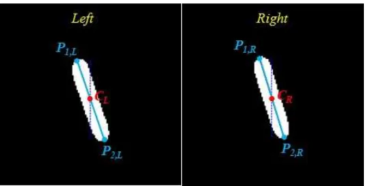
where h denotes the thresholded stereo image, and u and v the horizontal and vertical pixel coordinates, respectively. Furthermore, for non-spherical solids, the boundaries were detected through the maximum intensity gradient principle suggested by Nishino et al. [30]. Then, the distance between every point of the perimeter with respect to all of the other ones was measured in order to find the points P1 and P2 denoted in Figure 3, whose distance between each other was the largest. The line segment represents the particle longest axis. In Figure 6, C, P1, and P2 are marked for a cylindrical particle.
Given the 2D pixel coordinates of any pair of stereo corresponding points, for instance (CL, CR), the computation of the 3D metric coordinates (XW,C, YW,C, ZW,C) of that point in the world reference frame involved the solution of the projective transformations between the projective space of each virtual camera and the real world, and the calculation of the geometry which links both cameras. Since the first requisite is met through the process of camera calibration, the methodology proposed by Zhang [31] for such purpose was followed here. For the second task, the so-called epipolar geometry established by the stereo system has to be determined, therefore, the procedure to find it recommended by Zhang [32] was applied in this research.
Opposite to the normal trend of working in the coordinate system of the left camera, in this work all of the 3D points were projected back from the left camera frame to the world reference frame OWXWYWZW. For every 3D point , in the left camera coordinate system, the back projection was done through the next equation
. = 1 , (18)
where . represents the point in the world reference frame, is the transpose of the rotation matrix between both coordinate systems, and C denotes the translation vector between the origin of both coordinate frames. Once all of the operations to obtain the three-dimensional coordinates of points C, P1, and P2, respectively, in the world frame were completed, the trajectory of the settling particle could easily be reconstructed. Additionally, the velocity at its centroid VP and the angular orientation were computed from the following equations
= ∆ (19)
7 where d corresponds to the distance traveled per time increment Δt, P1P2 indicates the
longest axis vector of the object, and VP is 3D the velocity vector. Equation (19)
represents the method of conventional single particle tracking velocimetry. In order to estimate the drag force exerted on the solid at each time, the next equation, suggested by Mandø and Rosendahl [17] to model the motion of a cylindrical particle of mass m
immersed in a given flow field u, was employed
= − + +12 ( − ) + (21)
where mf denotes the mass of fluid displaced by the particle, and the gravity acceleration vector. The left side of Equation (21) represents the particle inertia, whilst the right side comprehends, in order, the buoyancy, pressure gradient, virtual mass acceleration, and any other force encompassed in F. Acknowledging that the fluid is at rest (u = 0) and that ⁄ corresponds to the acceleration vector and that mf is equal to the particle density times its volume, Equation (21) was reduced to
1 + 2 − 1 − = (22)
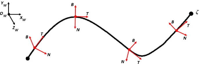
which, in turn, could be re-stated in terms of the tangential T, normal N, and binormal B unit vectors of a Frenet reference frame attached to trajectory of the particle as illustrated in Figure 7. Consequently, the next equations resulted
1 + 2 − 1 − = (23)
1 + 2 − 1 − = (24)
− 1 − = (25)
where FT, FN, and FB are the components of F in the tangential, normal, and binormal directions, respectively. Likewise, , , and are the components of in the same directions. Since the kinematics of the particle can be fully resolved within the Frenet frame as long as the 3D centroid-trajectory coordinates are known, the election of this procedure seemed natural according to Veldhuis et. al. [23]. In fact, Equations (23) to (25) were also used by them in their study of freely rising spheres. Moreover, they proposed too that the drag force vector can be determined as
= (26)
Being AP the area projected by the solid in a direction perpendicular to the drag force, the coefficient of resistance CD was calculated employing the following equation
=
8 In summary, through the application of Equations (19), (20), (26), and (27) the particle motion parameters relevant for this investigation were determined. Furthermore, the projected area for the cylinders was computed as = + 0.25 whilst for the disks it was calculated as = 0.25 + . For spheres, is simply the area of a circle with equal diameter.
3. Results
3.1 Spheres
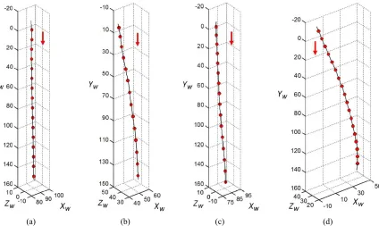
The 3D centroid trajectory of sphere S2 falling in mixture 80/20 at ReP = 15 is shown in Figure 8a. The red points highlight the 3D positions of the centroid. It can be seen that the trajectory was almost a vertical straight line provided that at these conditions both the flow around the particle and the wake were highly symmetrical, as illustrated in Figure 1a. Nevertheless, as ReP increased the symmetry was lost and the single trail became double and wavy (Figure 1b), thus deviating the 3D path significantly, as portrayed in Figure 8b for sphere S1 settling in water at ReP = 277.
With further increments of ReP the process of vortex shedding in the form of the so-called hairpin structures was noticed, as depicted in Figure 1c for the drop of sphere S5 in water at ReP = 902. This result is contrary to what Magarvey and Bishop [10] reported, because they said that the presence of such structures ends at ReP ~ 700. A typical fall path at this regime is provided in Figure 8c for sphere S4 sinking in mixture 65/35 at ReP = 656. At
ReP > 1000, in this research it was found that the wakes described by the spheres were entirely turbulent and asymmetrical, like the one shown in Figure 1d for sphere S11 descending in water at ReP = 4939. The corresponding 3D plot is given in Figure 8d, where a path largely deviated from a straight vertical line can be noticed.
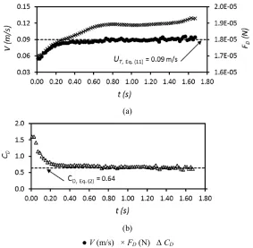
The change of velocity, drag force, and drag coefficient with time for sphere S1 sinking in water at ReP = 277 can be observed in Figure 9. Similar plots were generated for all the other spheres studied. From Figure 9a it was noticed that after t = 0.70 s the velocity stabilized at UT = 0.090 m/s, coinciding then with the prediction of Equation (11). The drag force remained approximately equal to FD = 1.9×10⁻⁵ N. From Figure 9b it was seen that also the coefficient of resistance attained a relatively stable value, CD = 0.66, just 3 % away from the estimation of Equation (2).
9 To investigate the uncertainty of the results, the drop of sphere S1 in water at Tf = 15 °C ( = 999.1 kg/m3, μ = 1.2×10⁻³ Pa∙s, ReP = 207) was repeated 9 times. The individual results achieved for UT and CD are shown in Table 5. Through the application of the error analysis procedure recommended by Taylor [33], the following outcome was obtained:
UT = 0.08 m/s + 1 % and CD = 0.79 + 1 %. Hence, suggesting that the uncertainty in the estimations of UT and CD, in general, was 1 %.
3.2 Cylinders
In Figure 11a it is depicted the free-fall of cylinder C4 in mixture 65/35 at ReP = 169. It can be observed that once the instabilities due to the dropping method were overcome, the path was relatively straight and the orientation was practically constant. However, for higher Reynolds numbers the trajectories exhibited some curvature and the oscillating secondary motion reported by Marchildon et al. [14] and Chow and Adams [8] was present, as it can be seen in Figures 11b and 11c for cylinders C6 and C2 sinking in mixtures 50/50 and 0/100 at ReP = 615 and ReP = 1975, respectively.
The patterns of fall can also be appreciated quantitatively from the corresponding 3D plots of Figure 11, where the blue line represents the cylinder longest axis location and the green points the positions of points P1 and P2, respectively. With the assistance of these plots it can be further accentuated that as the particle Reynolds number rises a cylindrical solid in free fall neither keeps a fixed orientation nor describes a linear trajectory. It is believed that the cause of this behavior is the fully turbulent flow structures developed at the rear of the particle, as illustrated in Figure 12 for the drop of cylinder C2 in water. Because of their high irregularity, the balance of the forces which keep the cylinder in a fixed position is lost, giving origin to torques which modify the particle orientation.
The time variation of the angle of incidence, projected area, velocity, drag force, and coefficient of resistance for the fall of cylinder C6 are plotted in Figure 13. It was observed that after t = 0.05 s, the angular change was noticeably symmetrical in the interval 68° < α < 88°. The variation of AP was similar though with opposite trend. Despite the oscillations, the velocity stabilized at UT = 0.32 m/s after t = 0.30 s. This magnitude of UT was 14 % larger than the estimation given by Equation (12). In general, for all the cases analyzed, once ReP surpassed 200, the magnitudes of UT obtained in this work were up to 17 % higher than the values predicted by Equation (12). It is thought that this is a consequence of the presence of the secondary motions.
Contrary to the behavior of VP, FD displayed a slight but continuous increase throughout the whole time interval, with FD = 2.1×10⁻³ N at the end of the recorded time. Nonetheless, the coefficient of resistance did reach the consistent value CD = 0.70 at final velocity conditions. Since the UT determined here was larger than the theoretical result, the corresponding value of CD was in consequence smaller than the one given by Equation (5) by 20 % approximately. This finding was consistent for all of the cases studied once
10 their equation they involved the influence of the secondary motions and the changes in angular orientation. In this case the dissimilarity remained below 11 %. Furthermore, the use of σ instead of ∅ as the shape descriptor for oscillating cylinders seemed to be an improved alternative.
3.3 Disks
The settling of disk D2 in mixture 80/20 at ReP = 20 is illustrated graphically in the 3D plot of Figure 15a. It was observed that at such low ReP the fall was steady with the maximum area of the disk projected perpendicular to the direction of motion, as reported by Stringham et al. [15]. Nonetheless, contrary to their assumption that the secondary motions for disks arise at ReP > 400, it was found here that they can appear at considerably lower values. For instance, tumbling was registered during the free-fall of disk D1 in mixture 65/35 at ReP = 226 (Figure 15b). The corresponding 2D representation is provided in Figure 2b. The secondary motions of gliding and oscillation were also witnessed in this work. Figures 2c, 15c, and 16 show the 2D, 3D, and Schlieren visualizations, respectively, of the oscillating fall of disk D3 in water at ReP = 1513. For clarity reasons the positions of the longest axis in Figure 15c were omitted. From the Schlieren images it was appreciated that the secondary motion, path deviations, and changes in orientation were also provoked by the irregular and turbulent patterns of flow developed in the vicinity of the particle, mainly at the rear.
The evolution of α, AP, VP, FD, and CD with time for tumbling disk D1 in mixture 65/35 at ReP = 226 is plotted in Figure 17, where it can be noticed that a highly consistent sinusoid-like variation affected all of the parameters. The range within which α moved was [10.5°, 81.7°]. Due to the regular oscillation observed, it was assumed that when the disk entered the field of view of the stereo system, it was already at steady state conditions, however, an explicit magnitude of terminal velocity could not be determined, instead an interval of variation was observed: 0.38 m/s < UT < 0.50 m/s. Moreover, it was also noticed that the prediction of Equation (12) coincided with the average of the experimental results of UT. The intervals of change described by the force and coefficient of drag were 0.7×10⁻³ N < FD < 4.9×10⁻³ N and 0.41 < CD < 1.86, respectively.
For the case of the oscillating disk D3 in water at ReP = 1513, the time-change of α, AP,
VP, FD, and CD, correspondingly, is given in Figure 18. The variation of the angle of incidence was significantly steady between 31.1° and 87.0°. AP also changed evenly. In addition, after t = 0.05 s, the peaks of velocity roughly agreed with the prediction of Equation (12). The differences did not exceed 11 %. Furthermore, VP, FD, and CD varied within the following intervals: 0.12 m/s < VP < 0.31 m/s, 0.5×10⁻³ N < FD < 4.2×10⁻³ N, and 0.32 < CD < 7.0. For the same range of ReP, the large values of CD achieved for this disk agreed with the data reported by reported by Stringham et al. [15].
11 Equation (5) was located within the minimum and maximum experimental results found here. Averages of CD were not calculated in this occasion provided that a strong argument supporting the veracity of this approach cannot be provided.
4. Relation between CD and α
In Figure 13a it can be seen that after reaching terminal velocity conditions, cylinder C6 falling in mixture 50/50 at ReP = 615 experienced a noticeable increase in α during the interval 0.29 s < t < 0.33 s, to then decrease for 0.33 s < t < 0.44 s, and increase again during 0.44 s < t < 0.52 s. If the values of CD are plotted versus α for the same time intervals, the influence of the angular orientation on the drag coefficient can be observed graphically, as illustrated in Figure 19. By following the same criteria, the α – CD plots of Figure 20 for cylinder C4 sinking in water at ReP = 1975 were obtained. In both cases, the sinusoidal approaches of Rosendahl [16], and Mandø and Rosendahl [17] were included for comparison.
From the experimental results plotted in Figures 19 and 20 it was observed that CD can either increase or decrease with α. A general explicit trend valid for all time intervals was not visualized. Moreover, despite the fact that the recommendation of Mandø and Rosendahl [17] showed a lower discrepancy with respect to the current work, both models failed to reproduce the tendency witnessed in each time-interval plot because they were designed in such a way that for every increment of α there always exists an increment of
CD. This assumption is typical of configurations were the particle motion is restricted.
Figure 21 contains the α – CD plots generated for two cases of disk D1 settling in mixture 65/35 at ReP = 226 and 237, respectively, and under the presence of tumble. It can be distinguished that in general CD increased with α, though not always describing the same tendency. In some of the graphs the rise was gradual, whilst in others it was abrupt. It is thought that the reason for such a behavior was the fact that the development of the secondary motion did not always follow the same history even for the same particle tested at equal conditions.
In Figure 22 the α – CD plots corresponding to the fall of disk D3 in water at ReP = 1513 and subjected to oscillatory motion are provided. In this case it was noticed too that CD
tended to augment with α. Additionally, either for a decreasing or increasing α, the tendency was similar. It can also be observed that the oscillating disk experienced higher resistance than the tumbling one. This because at pure oscillation, the largest projected area of the disk is exposed perpendicularly to the motion direction a larger number of times.
12
5. Conclusions
A new image-based methodology to analyze the settling motion of spherical and non-spherical particles in a fluid at 0.3 < ReP < 5000 was proposed. For each solid the 3D centroid-displacement trajectory and kinematics were determined through single-camera stereo vision and conventional PTV, respectively; the drag force was estimated by means of a Frenet frame of reference which moved along the settling path, and the changes in orientation were resolved through the computation of the angle of incidence and used to calculate the instantaneous true projected area at every position for the drag coefficient calculations. Furthermore, insight on the flow structures surrounding the solids at selected
ReP was gained with the assistance of Z-type Schlieren visualization in water.
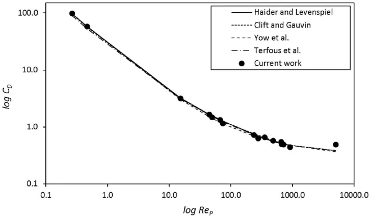
For spherical particles, it was observed that the evolution of the neighboring fluid structures deviated the fall paths from vertical lines, nevertheless, it did not stop the solids from reaching stable values of UT and CD. It was also noticed that the hairpin-pattern of vortex shedding can endure up to ReP ~ 900, contrary to what has been reported before. Moreover, by comparing the experimental results of CD against existing drag correlations for spheres, a close agreement was obtained, therefore validating the methodology proposed in this study.
For disks and cylinders a steady fall with the maximum projected area perpendicular to the direction of motion was seen up to ReP ~ 163 and 240, respectively. As ReP augmented, it was witnessed that the particles exhibited regular oscillations during their descent, and for the disks, also tumbling. Both secondary motions provoked a fully turbulent behavior in the surrounding flow as well as in the wake, which in turn diverted the settling paths far from straight lines, and generated angular variations. Because the oscillation of the cylinders did not produce large changes in α, steady values of UT and CD could be noticed, nonetheless an opposite result was obtained for the oscillating and tumbling disks. Additionally, with respect to published drag correlations, a significant disagreement was attained for the cases where secondary motions existed, thus confirming their influence on CD. This also reinforced the importance of preserving the particle-fluid interaction undisturbed during the tests. Although a clear relation between CD and α was not perceived, plots based on experimental data evidencing the impact of α on CD were generated for the first time and can be used to strengthen the drag numerical models available in the literature.
Acknowledgements
The authors of this work would like to give thanks to the Mexican Council for Research and Technology, CONACYT, for the economic support given to this project.
References
[1] R. Clift and W. Gauvin, "Motion of entrained particles in gas streams", Can. J. Chem. Eng., vol. 49, no. 4, pp. 439-448, 1971.
13 [3] H. Yow, M. Pitt and A. Salman, "Drag correlations for particles of regular shape",
Advanced Powder Technology, vol. 16, no. 4, pp. 363-372, 2005.
[4] A. Terfous, A. Hazzab and A. Ghenaim, "Predicting the drag coefficient and settling velocity of spherical particles", Powder Technology, vol. 239, pp. 12-20, 2013. [5] G. Ganser, "A rational approach to drag prediction of spherical and nonspherical
particles", Powder Technology, vol. 77, no. 2, pp. 143-152, 1993.
[6] R. Chhabra, L. Agarwal and N. Sinha, "Drag on non-spherical particles: an evaluation of available methods", Powder Technology, vol. 101, no. 3, pp. 288-295, 1999.
[7] A. Hölzer and M. Sommerfeld, "New simple correlation formula for the drag coefficient of non-spherical particles", Powder Technology, vol. 184, no. 3, pp. 361-365, 2008.
[8] A. Chow and E. Adams, "Prediction of Drag Coefficient and Secondary Motion of Free-Falling Rigid Cylindrical Particles with and without Curvature at Moderate Reynolds Number", Journal of Hydraulic Engineering, vol. 137, no. 11, pp. 1406-1414, 2011.
[9] H. Wadell, "The coefficient of resistance as a function of Reynolds number for solids of various shapes", Journal of the Franklin Institute, vol. 217, no. 4, pp. 459-490, 1934.
[10] R. Magarvey and R. Bishop, "Transition ranges for three-dimensional wakes", Can. J. Phys., vol. 39, no. 10, pp. 1418-1422, 1961.
[11] R. Magarvey and C. MacLatchy, "Vortices in sphere wakes", Canadian Journal of Physics, vol. 43, no. 9, pp. 1649-1656, 1965.
[12] C. Veldhuis, A. Biesheuvel, L. Wijngaarden and D. Lohse, "Motion and wake structure of spherical particles", Nonlinearity, vol. 18, no. 1, pp. C1-C8, 2004. [13] C. Veldhuis and A. Biesheuvel, "An experimental study of the regimes of motion
of spheres falling or ascending freely in a Newtonian fluid", International Journal of Multiphase Flow, vol. 33, no. 10, pp. 1074-1087, 2007.
[14] E. Marchildon, A. Clamen and W. Gauvin, "Drag and oscillatory motion of freely falling cylindrical particles", Can. J. Chem. Eng., vol. 42, no. 4, pp. 178-182, 1964. [15] G. E. Stringham, D. B. Simons, and H. P. Guy, "The behaviour of large particles falling in quiescent liquids," U.S. Department of the Interior. Washington D.C.: 1969, pp. 4-43.
[16] L. Rosendahl, "Using a multi-parameter particle shape description to predict the motion of non-spherical particle shapes in swirling flow", Applied Mathematical Modelling, vol. 24, no. 1, pp. 11-25, 2000.
[17] M. Mandø and L. Rosendahl, "On the motion of non-spherical particles at high Reynolds number", Powder Technology, vol. 202, no. 1-3, pp. 1-13, 2010.
[18] M. Zastawny, G. Mallouppas, F. Zhao and B. van Wachem, "Derivation of drag and lift force and torque coefficients for non-spherical particles in flows", International Journal of Multiphase Flow, vol. 39, pp. 227-239, 2012. [19] W. Ng and Y. Zhang, "Stereoscopic imaging and reconstruction of the 3D geometry
of flame surfaces", Exp Fluids, vol. 34, no. 4, pp. 484-493, 2003.
14 [21] T. Xue, L. Qu, Z. Cao and T. Zhang, "Three-dimensional feature parameters measurement of bubbles in gas–liquid two-phase flow based on virtual stereo vision", Flow Measurement and Instrumentation, vol. 27, pp. 29-36, 2012.
[22] R. Wang, X. Li and Y. Zhang, "Analysis and optimization of the stereo-system with a four-mirror adapter", Journal of the European Optical Society: Rapid Publications, vol. 3, 2008.
[23] C. Veldhuis, A. Biesheuvel and D. Lohse, "Freely rising light solid spheres", International Journal of Multiphase Flow, vol. 35, no. 4, pp. 312-322, 2009.
[24] G. G. Marcus, S. Parsa, S. kramel, R. Ni and G. A. Voth, "Measurements of the solid-body rotation of anisotropic particles in 3D turbulence", New Journal of Physics, vol. 16, no. 10, pp. 102001, 2014.
[25] B. Krueger, S. Wirtz and V. Scherer, "Measurement of drag coefficients of non-spherical particles with a camera-based method", Powder Technology, vol. 278, pp. 157-170, 2015.
[26] S. T. Barnard and M. A. Fischler, "Computational stereo", SRI International, Menlo Park, California, 1982.
[27] H. Fiedler, K. Nottmeyer, P. Wegener and S. Raghu, "Schlieren photography of water flow", Experiments in Fluids, vol. 3, no. 3, pp. 145-151, 1985.
[28] Physical properties of glycerine and its solutions. Glycerine Producers Association, 1963.
[29] N. Otsu, "A Threshold Selection Method from Gray-Level Histograms", IEEE Transactions on Systems, Man, and Cybernetics, vol. 9, no. 1, pp. 62-66, 1979. [30] K. Nishino, H. Kato and K. Torii, "Stereo imaging for simultaneous measurement
of size and velocity of particles in dispersed two-phase flow", Measurement Science and Technology, vol. 11, no. 6, pp. 633-645, 2000.
[31] Z. Zhang, "A flexible new technique for camera calibration", IEEE Transactions on Pattern Analysis and Machine Intelligence, vol. 22, no. 11, pp. 1330-1334, 2000. [32] Z. Zhang, "Motion and structure from two perspective views: from essential parameters to Euclidean motion through the fundamental matrix", Journal of the Optical Society of America A, vol. 14, no. 11, p. 2938, 1997.
[33] J. R. Taylor, An introduction to error analysis. The study of uncertainties in physical measurements, second ed. University Science Books, USA, 1997.
Vitae
15
(a) (b)
[image:17.612.110.503.68.394.2](c) (d)
Figure 1 (a) Stable wake behind a 7.9 mm PTFE sphere, ReP = 43; (b) hairpin vortex structure of a
(a) (b) (c)
Figure 2 (a) Regular oscillations of a 4.0×8.3 mm PTFE sinking cylinder, ReP = 406; (b) tumbling fall
Figure 6 Detected centroid C and extreme points P1 and P2 on both sides of the stereo image of a
cylindrical particle.
(a) (b) (c) (d)
Figure 8 3D plots of the centroid trajectory of settling spheres: S2 in mixture 80/20, ReP = 15 (a), S1
in water, ReP = 277 (b), S4 in mixture 65/35, ReP = 656 (c), and S11 in water, ReP = 4939 (d),
respectively.
(a)
(b)
[image:25.612.163.446.69.346.2]● V (m/s) × FD (N) Δ CD
(a) (b) (c)
Figure 11 2D visualizations and 3D centroid trajectories of the settling cylinders: C4 in mixture
65/35, ReP = 169 (a), C6 in mixture 50/50, ReP = 615 (b), and C2 in water ReP = 1975 (c),
respectively. The blue lines denote the location of the longest axis, and the green dots the position of points P1 and P2, respectively.
(a)
(b)
(c)
[image:29.612.164.446.67.473.2]▪α (°) ◊ AP (m2) ● V (m/s) × FD (N) Δ CD
Figure 13 Time variation of α and AP (a), V and FD (b), and CD (c) for the fall cylinder C6 in mixture
(a) (b) (c)
Figure 15 3D plots of the centroid path of falling disks: D2 in mixture 80/20, ReP = 20 (a), D1 in
mixture 65/35, ReP = 226 (b), D3 in water, ReP = 1513 (c), respectively. The blue lines denote the
position of the longest axis, and the green dots the position of points P1 and P2, respectively; but for
clarity reasons they were omitted in plot (c).
(a)
(b)
(c)
[image:33.612.163.447.67.478.2]▪α (°) ◊ AP (m2) ● V (m/s) × FD (N) Δ CD
Figure 17 Time variation of α and AP (a), V and FD (b), and CD (c) during the sinking of disk D1 in
(a)
(b)
(c)
[image:34.612.164.447.68.482.2]▪α (°) ◊ AP (m2) ● V (m/s) × FD (N) Δ CD
Figure 18 Time variation of α and AP (a), V and FD (b), and CD (c) during the settling of disk D3 in
Increasing α
0.29 s < t < 0.33 s 0.33 s <Decreasing t < 0.44 s α
(a) (b)
Increasing α
0.44 s < t < 0.52 s
(c)
[image:35.612.113.498.66.368.2]● Current work Δ Rosendahl × Mandø and Rosendahl
Figure 19 Variation of CD with respect to α at UT conditions during the fall of cylinder C6 in mixture
Increasing α
0.19 s < t < 0.30 s 0.30 s <Decreasing t < 0.34 s α
(a) (b)
Increasing α
0.34 s < t < 0.38 s 0.38 s <Decreasing t < 0.47 s α
(c) (d)
[image:36.612.111.502.66.383.2]● Current work Δ Rosendahl × Mandø and Rosendahl
Figure 20 Variation of CD with respect to α at UT conditions during the settling of cylinder C4 water,
Decreasing α Increasing α
● 0.02 s < t < 0.06 s
× 0.10 s < t < 0.13 s Δ 0.17 s <* 0.24 s < t t < 0.27 s < 0.20 s ● 0.06 s <× 0.13 s < t t < 0.13 s < 0.17 s Δ 0.20 s < t < 0.24 s
(a) (b)
Increasing α Decreasing α
● 0.03 s < t < 0.07 s
× 0.14 s < t < 0.16 s Δ 0.20 s <* 0.28 s < t t < 0.31 s < 0.25 s ● 0.07 s <× 0.16 s < t t < 0.14 s < 0.20 s Δ 0.25 s < t < 0.28 s
[image:37.612.107.505.72.388.2](c) (d)
Figure 21 Variation of CD with respect to α at UT conditions for the fall of disk D1 in mixture 65/35,
at ReP = 226 (a,b) and ReP = 237 (c,d), respectively. For (a) and (d) α decreased with t, for (b) and (c)
Decreasing α Increasing α
● 0.04 s < t < 0.11 s
× 0.18 s < t < 0.25 s Δ 0.32 s < t < 0.37 s ● 0.11 s <× 0.25 s < t t < 0.32 s < 0.18 s
[image:38.612.109.500.64.228.2](a) (b)
Figure 22 Variation of CD with respect to α at UT conditions during the drop of disk D3 in water, at
Table 1Some representative correlations published in the literature to estimate de drag coefficient of spherical particles in free-fall.
Year Author Equation
1970 Gauvin [1] Clift and = 24 1 + 0.15 . +1 + 4.25×100.42 .
< 10
(1)
1989 Haider and Levenspiel [2]
= 24 1 + 0.1806 . + 0.4251
1 + 6880.95 < 2.6×10
(2)
2005 Yow et al. [3] = 0.3 +
23.5 + 4.6
< 2×10
(3)
2013 Terfous et al. [4] = 2.689 +21.683+0.131−10.616. +12.216.
0.1 < < 5×10
Table 2Some typical drag correlations found in the literature to estimate the drag coefficient of non-spherical particles in free-fall.
Year Author Equation
1989 Haider and Levenspiel [2]
= 24 1 + 8.1716 . ∅ . . ∅
+73.69+ 5.378 .. ∅∅
Isometric particles, < 2.5×10 , ∅ ≥ 0.67
(5)
1993 Ganser [5, 6]
= 24 [1 + 0.1118( ) . ]
+ 0.4305
1 + 3305
= + √∅ ; = 10 . ( ∅).
Isometric particles, < 10
(6)
2008 Hölzer and
Sommer-feld [7] = 8 ∅∥+ 16 √∅+ 3 ∅ / +
0.4210 . ( ∅) . ∅
< 10
(7)
2011 Chow and Adams [8]
=12 1 + < 1.5
=2 > 1.5
Cylinders, 200 < < 6000
Table 3 Dimensions and materials of the particles.
Shape d (mm) L (mm) Ø Material Name
Sphere
3.0 - 1.0 Nyloni S1
4.8 - 1.0 PTFEii S2
5.0 - 1.0 Brassiii S3
6.0 - 1.0 Brass S4
6.4 - 1.0 Nylon S5
6.4 - 1.0 PTFE S6
6.4 - 1.0 Brass S7
7.0 - 1.0 Aluminiumiv S8
7.9 - 1.0 PTFE S9
9.0 - 1.0 Brass S10
9.5 - 1.0 PTFE S11
Cylinder
5.0 10.2 0.8 Brass C1
4.0 8.3 0.8 PTFE C2
4.0 9.2 0.8 PTFE C3
4.0 10.4 0.8 PTFE C4
4.0 20.2 0.7 PTFE C5
5.0 10.4 0.8 PTFE C6
5.0 20.3 0.7 PTFE C7
Disk 6.0 6.4 1.6 2.5 0.7 0.8 Aluminium Brass D1 D2
10.0 2.9 0.7 PTFE D3
Table 4Matrix of experiments. The fluid properties were taken from the Glycerin Producers Association [28] and textbook thermodynamic tables.
%weight
Glyc. / Water Tf (°C) (kg/m3) μ (Pa∙s) Particles Dropped
100/0 20 1261.1 1.400 S3, S4, C1
80/20 25 1205.5 0.047 S2, S3, S8, S9, S11, C2, C4, C6, D2
65/35 30 1162.0 0.010 C4 – C7, D1 – D3 S3, S4, S6 – S8,
50/50 30 1121.1 0.004 S6, C2, C3, C6, D3
Table 5Results of the repeatability test done with sphere S1 settling in pure water at ReP = 207.
N UT (m/s) CD N UT (m/s) CD N UT (m/s) CD
Table 6Some representative values of the drag coefficient obtained for the settling disks.
Secondary motions were not present
% wt.
Glyc./Water Particle UT (m/s) ReP CD CD, Eq (5)
80/20 D2 0.15 20 2.90 3.24
65/35 D2 0.26 163 1.0 1.14
Secondary motions were present
% wt.
Glyc./Water Particle UT ~ VP,average (m/s) ReP CD, min CD, max CD, Eq (5) 65/35 D1 D3 0.44 0.21 226 187 0.41 0.94 1.86 1.58 1.54 1.38
50/50 D3 0.20 425 0.54 3.54 1.43