EQ5DMAP: a command for mapping between EQ-5D-3L and EQ-5D-5L

(1)

EQ-5D-5L

.

White Rose Research Online URL for this paper:

http://eprints.whiterose.ac.uk/124872/

Version: Published Version

Article:

Hernandez, M. orcid.org/0000-0003-4474-5883 and Pudney, S. (2018) EQ5DMAP: a

command for mapping between EQ-5D-3L and EQ-5D-5L. The Stata journal, 18 (2). pp.

395-415. ISSN 1536-867X

Notwithstanding the Stata Journal copyright notice, StataCorp and the Stata Journal

hereby agree that an electronic copy (PDF) of the following article can be made available

by open access: Hernandez-Alava, M., and S. Pudney. 2018 "eq5dmap: A command for

mapping between EQ-5D-3L and EQ-5D-5L". Stata Journal 18: 395-415. The Stata

Journal website: https://www.stata-journal.com

[email protected] https://eprints.whiterose.ac.uk/ Reuse

See Attached

Takedown

If you consider content in White Rose Research Online to be in breach of UK law, please notify us by

(2)

Editors

H. Joseph Newton

Department of Statistics Texas A&M University College Station, Texas [email protected]

Nicholas J. Cox

Department of Geography Durham University Durham, UK

[email protected]

Associate Editors

Christopher F. Baum, Boston College

Nathaniel Beck, New York University

Rino Bellocco, Karolinska Institutet, Sweden, and University of Milano-Bicocca, Italy

Maarten L. Buis, University of Konstanz, Germany

A. Colin Cameron, University of California–Davis

Mario A. Cleves, University of Arkansas for Medical Sciences

Michael Crowther, University of Leicester, UK

William D. Dupont, Vanderbilt University

Philip Ender, University of California–Los Angeles

James Hardin, University of South Carolina

Ben Jann, University of Bern, Switzerland

Stephen Jenkins, London School of Economics and Political Science

Ulrich Kohler, University of Potsdam, Germany

Frauke Kreuter, Univ. of Maryland–College Park

Peter A. Lachenbruch, Oregon State University

Stanley Lemeshow, Ohio State University

J. Scott Long, Indiana University

Roger Newson, Imperial College, London

Austin Nichols, Abt Associates, Washington, DC

Marcello Pagano, Harvard School of Public Health

Sophia Rabe-Hesketh, Univ. of California–Berkeley

J. Patrick Royston, MRC CTU at UCL, London, UK

Mark E. Schaffer, Heriot-Watt Univ., Edinburgh

Philippe Van Kerm, LISER, Luxembourg

Vincenzo Verardi, Universit´e Libre de Bruxelles, Belgium

Ian White, MRC CTU at UCL, London, UK

Richard A. Williams, University of Notre Dame

Jeffrey Wooldridge, Michigan State University

Stata Press Editorial Manager

Lisa Gilmore

Stata Press Copy Editors

Adam Crawley,David Culwell, andDeirdre Skaggs

TheStata Journalpublishes reviewed papers together with shorter notes or comments, regular columns, book reviews, and other material of interest to Stata users. Examples of the types of papers include 1) expository papers that link the use of Stata commands or programs to associated principles, such as those that will serve as tutorials for users first encountering a new field of statistics or a major new technique; 2) papers that go “beyond the Stata manual” in explaining key features or uses of Stata that are of interest to intermediate or advanced users of Stata; 3) papers that discuss new commands or Stata programs of interest either to a wide spectrum of users (e.g., in data management or graphics) or to some large segment of Stata users (e.g., in survey statistics, survival analysis, panel analysis, or limited dependent variable modeling); 4) papers analyzing the statistical properties of new or existing estimators and tests in Stata; 5) papers that could be of interest or usefulness to researchers, especially in fields that are of practical importance but are not often included in texts or other journals, such as the use of Stata in managing datasets, especially large datasets, with advice from hard-won experience; and 6) papers of interest to those who teach, including Stata with topics such as extended examples of techniques and interpretation of results, simulations of statistical concepts, and overviews of subject areas.

TheStata Journalis indexed and abstracted byCompuMath Citation Index,Current Contents/Social and Behav-ioral Sciences,RePEc: Research Papers in Economics,Science Citation Index Expanded(also known asSciSearch),

Scopus, andSocial Sciences Citation Index.

For more information on theStata Journal, including information for authors, see the webpage

(3)

http://www.stata.com/bookstore/sj.html

Subscription rateslisted below include both a printed and an electronic copy unless otherwise mentioned.

U.S. and Canada Elsewhere

Printed & electronic Printed & electronic

1-year subscription $124 1-year subscription $154 2-year subscription $224 2-year subscription $284 3-year subscription $310 3-year subscription $400

1-year student subscription $ 89 1-year student subscription $119

1-year institutional subscription $375 1-year institutional subscription $405 2-year institutional subscription $679 2-year institutional subscription $739 3-year institutional subscription $935 3-year institutional subscription $1,025

Electronic only Electronic only

1-year subscription $ 89 1-year subscription $ 89 2-year subscription $162 2-year subscription $162 3-year subscription $229 3-year subscription $229

1-year student subscription $ 62 1-year student subscription $ 62

Back issues of theStata Journalmay be ordered online at

http://www.stata.com/bookstore/sjj.html

Individual articles three or more years old may be accessed online without charge. More recent articles may be ordered online.

http://www.stata-journal.com/archives.html

TheStata Journalis published quarterly by the Stata Press, College Station, Texas, USA.

Address changes should be sent to the Stata Journal, StataCorp, 4905 Lakeway Drive, College Station, TX 77845, USA, or emailed to [email protected].

® ®

Copyright c2018 by StataCorp LLC

Copyright Statement: TheStata Journaland the contents of the supporting files (programs, datasets, and help files) are copyright cby StataCorp LLC. The contents of the supporting files (programs, datasets, and help files) may be copied or reproduced by any means whatsoever, in whole or in part, as long as any copy or reproduction includes attribution to both (1) the author and (2) theStata Journal.

The articles appearing in theStata Journalmay be copied or reproduced as printed copies, in whole or in part, as long as any copy or reproduction includes attribution to both (1) the author and (2) theStata Journal. Written permission must be obtained from StataCorp if you wish to make electronic copies of the insertions. This precludes placing electronic copies of theStata Journal, in whole or in part, on publicly accessible websites, fileservers, or other locations where the copy may be accessed by anyone other than the subscriber. Users of any of the software, ideas, data, or other materials published in theStata Journalor the supporting files understand that such use is made without warranty of any kind, by either theStata Journal, the author, or StataCorp. In particular, there is no warranty of fitness of purpose or merchantability, nor for special, incidental, or consequential damages such as loss of profits. The purpose of theStata Journalis to promote free communication among Stata users.

(4)

eq5dmap: A command for mapping between

EQ-5D-3L and EQ-5D-5L

M´onica Hern´andez-Alava School of Health and Related Research Health Economics and Decision Science

University of Sheffield

Sheffield,UK

[email protected]

Stephen Pudney

School of Health and Related Research Health Economics and Decision Science

University of Sheffield

Sheffield,UK

[email protected]

Abstract. In this article, we describe a new command,eq5dmap, for conditional prediction of the utility values of EQ-5D-5L (EQ-5D-3L) from observed or speci-fied values of EQ-5D-3L (EQ-5D-5L) conditional on age and gender. Predictions can be made either from the five-item health descriptions or from the (exact or approximate) utility score. The prediction process is based on a joint statistical model of the two variants of EQ-5D that have been fit to alternative reference datasets (the National Data Bank for Rheumatic Diseases and a EuroQol Group coordinated data-collection study). The underlying model is a system of ordinal regressions with a flexible residual distribution specified as Gaussian or as a copula mixture. Use of the command is illustrated with an application that includes an investigation of the sensitivity of the mapping outcomes to the choice of reference dataset.

Keywords: st0528, eq5dmap,EQ-5D,EQ-5D-3L,EQ-5D-5L, mapping, conditional prediction, copula, mixture model

1 Introduction

The quality-adjusted life year (QALY) is one of the most widely used health benefit

mea-sures in economic evaluations of interventions, services, or programs designed to improve

health. TheQALYallows healthcare decision makers to use a consistent approach across

a broad range of disease areas, treatments, and patients. It is the preferred outcome measure for the National Institute for Health and Care Excellence in its appraisals of

health interventions in England (NICE 2014). Preference-based measures such as the

EQ-5D-3L underpin the calculation ofQALYs.

EQ-5Ddescribes health states in terms of five dimensions: mobility, self-care, usual

activities, pain or discomfort, and anxiety or depression. The original EQ-5D, now

called EQ-5D-3L, measures each dimension on a three-level scale (no problems, some

or moderate problems, extreme problems). EQ-5D-3L can describe 243 different health

states in this way. For example, the health state 11223 corresponds to no problems in the mobility and self-care dimensions, some problems in the usual activities and pain or discomfort dimensions, and extreme problems in the anxiety or depression dimension. Valuation studies in different countries assigned an index or utility score to each of the

c

(5)

health states described in this way. Dolan (1997) published the firstUKvalue set using general public preferences. Other countries have developed their own value sets, but in all countries, the health state 11111 (full health) is assigned a utility score of 1, and death is assigned a value of 0. States with utility scores between 0 and 1 reflect some degree of impairment, and states with negative valuations are considered worse than death.

A new version of the health description system, theEQ-5D-5L, has been developed to

try to address concerns about the lack of sensitivity and floor or ceiling distortions of the

EQ-5D-3L. The number of dimensions has remained unchanged, but the new EQ-5D-5L

extends the number of levels per dimension from three to five (no problems, slight prob-lems, moderate probprob-lems, severe probprob-lems, extreme problems). To improve consistency

across dimensions and aid understanding, there have also been some wording changes.1

The number of discrete health states described by the new version is 3,125. Utility

value sets for EQ-5D-5L have been released for England (Devlin et al. 2018),2 _Japan

(Shiroiwa et al. 2016), Canada (Xie et al. 2016), Uruguay (Augustovski et al. 2016), Netherlands (Versteegh et al. 2016), Korea (Kim et al. 2016), China (Luo et al. 2017), and Indonesia (Purba et al. 2017), and similar work is underway in other countries.

Many studies now includeEQ-5D-5Linstead of the originalEQ-5D-3L. We have shown

in previous articles (Hern´andez-Alava and Pudney 2017; Hern´andez-Alava et al. 2018)

that in the UK, EQ-5D-3L and EQ-5D-5L lead to different utility scores for the same

underlying level of health; this has profound implications for economic evaluations. It is, therefore, inappropriate to mix the evidence collected using both instruments without adjusting for these differences. Because all studies, new and those previously completed, will form part of the available evidence in future economic evaluations, it is important to have a consistent way of translating health benefits measured using one of the two

versions of EQ-5D into the other. Hern´andez-Alava and Pudney (2017) developed a

flexible model that allows analysis of the joint responses to EQ-5D-3L and EQ-5D-5L.

The underlying model is a system of ordinal regressions with a flexible copula-mixture residual distribution. This model has been refit using two different datasets and results reported elsewhere (Hern´andez-Alava et al. 2018). In this article, we describe a new

command, eq5dmap, for conditional prediction of theEQ-5D-5L (EQ-5D-3L) utility from

observedEQ-5D-3L (EQ-5D-5L) responses or specified utility values and age and gender.

The command predictions are based on the models in Hern´andez-Alava et al. (2018).

This command is the only available method of translating evidence from EQ-5D-3L to

EQ-5D-5Land vice versa using the individual health states, an individual utility value, or an approximate utility score. Section 2 describes the two types of predictions that can be computed with the command. Section 3 explains briefly the underlying statistical model. The command syntax is fully described in section 4. Section 5 presents an illustrative example of the use of the command. Section 6 concludes.

1. See the EuroQol website https://euroqol.org/eq-5d-instruments/ for examples of the question word-ing used in EQ-5D-3L and EQ-5D-5L.

(6)

2 The mapping method

Theeq5dmapcommand allows mapping both from the older to the newer format (3L→

5L) and the reverse (5L→3L). We explain the mapping methodology for the case of

3L→5L, but the procedure is essentially the same for 5L→3L.

Let Y3d ∈ {1,2,3} and Y5d ∈ {1,2,3,4,5} represent outcomes for the dth

do-main (d= 1, . . . ,5) of EQ-5D-3L and EQ-5D-5L, respectively. Define the vectors Y3 =

(Y31, . . . , Y35) and Y5 = (Y51, . . . , Y55) , and write the corresponding utility scoring

scalesυ3(.) and υ5(.). Our aim is to calculate the expectation of υ5(Y5) conditional

on the values of a vector of covariatesX and also on available information aboutY3.

Depending on the form of that information, two types of mapping can be done.

2.1 A specified value for

Y

3

LetS5={1, . . . ,5}5 be the set of possible values that can be taken by the vector Y5.

If we know the conditioning value ofY3, the expectation ofυ5 can be computed as

E(υ5|Y3=y3,X) =

X

y5∈S5

υ5(y5)p(y5|y3,X)

wherep(y5|y3,X) is the form of conditional probability implied by the specified

under-lying statistical model for the joint distributionY3|X andY5|X.

2.2 A specified (approximate) value for

υ

3

(

Y

3

)

In some cases, the user may know only the value of υ3(Y3), rather than Y3 itself.

Because the mapping Y3 → υ3 is not (quite) one to one, this case involves weaker

conditioning information. Another possibility is that the user has only a predicted

valueυb3, and the prediction may not correspond precisely to any validEQ-5D-3Lutility

score. We handle both problems by distance-weighted averaging within a neighborhood

of the specified value,υb3.

LetCbe a user-specified bandwidth. Define a set of vectors

S(υ) ={Y3 : |υ3(Y3)−υ| ≤C}

and a weight function of Epanechnikov form:

ω(υ3−υ) =

(

1− {(υ3−υ)/C}2

for|(υ3−υ)|< C

0 otherwise

The estimate of the expected value ofυ5is

P

y3∈S(bυ3)

ω{υ3(y3)−bυ3} P

y5

υ5(y5)p(y5|y3,X)

P

y3∈S(υb3)

(7)

where the summation overy5covers all 3,125 possible outcome vectors for theEQ-5D-5L

descriptive system.

3 The underlying statistical model

The predictive distribution Pr(Y5|Y3,X) is derived from a model of the joint

distri-bution ofY3|X and Y5|X developed by Hern´andez-Alava and Pudney (2017). That

model is a system of 10 latent regressions, arranged in 5 groups, following the natural

pairing of the dimensions in the 2 versions of EQ-5D, with domain d containing the

equations forY3d andY5d,

Y∗

3d = Xβ3d+U3d Y∗

5d = Xβ5d+U5d

)

d= 1, . . . ,5

wherei indexes individual cases and we assume random sampling so that all sampled

variables are independent across individuals. X is a row vector of covariates, andβ₃d

and β₅d are column vectors of coefficients conformable withX. We assume that the

covariate vectorX is the same for both the three-level and the five-level version of the

rth domain but may differ between domains. U3d and U5d are unobserved residuals,

which may be stochastically dependent and nonnormal. The latent dependent variables

Y∗

3d and Y5∗d are not observed directly, but they have observable ordinal counterparts,

Y3d andY5d, that are generated by the threshold-crossing conditions

Ykd=q iff Γkqd≤Ykd∗ <Γk(q+1)d, q= 1, . . . , Qk, and k= 3,5

where Qk = 3 or 5 is the number of categories of Ykd and the Γkqd are threshold

pa-rameters, with Γk1d=−∞and Γk(Qk+1)d= +∞.

To allow for background correlation between the five dimensions of EQ-5D, we

de-compose the residualUkid into a single between-group factor Vi, which represents the

individual’s general tendency to give more or less positive responses and a specific

resid-ualεkid correlated within but not between dimensions,

Ukid=ψkdVi+εkid k= 3,5 and d= 1, . . . ,5

where theψkd are a set of 10 parameters.

The model can be fit under various alternative assumptions about the joint

distribu-tion of the residualsε3id andε5id within each dimension dand the distributional form

of the common factorVi. The eq5dmap command offers two specifications: the

Gaus-sian, where the pairsε3id andε5idhave bivariate normal distributions andVi∼N(0,1);

and the copula specification, where the distribution of each pairε3id andε5id is

spec-ified in copula form with normal mixture marginals and Vi as a normal mixture (see

Hern´andez-Alava and Pudney [2017] for details).

(8)

of study. We present a concise summary of both datasets below. A more detailed discussion of the similarities and differences between the two datasets can be found

in Pennington et al. (Forthcoming). Users of eq5dmapshould consider carefully which

reference dataset is better suited for their study.

The first dataset comes from the National Data Bank for Rheumatic Diseases (NDB),

which is a register of patients with rheumatic disease, mainly referred by U.S. and Canadian rheumatologists (Wolfe and Michaud 2011). In 2011, there was a switch from

the three-level to the five-level version of EQ-5D, and both versions were collected in

parallel during the January 2011 wave, which we used to fit the reference model. The second dataset comes from a data-collection study coordinated and partly funded by

the EuroQuol Group (EQG) between August 2009 and September 2010, in six countries:

Denmark, England, Italy, the Netherlands, Poland, and Scotland. It covered eight broad patient groups (cardiovascular disease, respiratory disease, depression, diabetes, liver disease, personality disorders, arthritis, and stroke) and a student cohort (healthy

population). ThisEQGdataset was intended to cover many responses across all the

EQ-5Ddimensions in a range of diseases (Janssen et al. 2013; van Hout et al. 2012). The

EQGsample is younger than theNDBsample, with an average age of 51 versus 63, and

it covers a wider age range. There is a big difference in gender composition: theEQG

sample is 53% female, compared with 81% for NDB, in line with what is expected in

a rheumatoid arthritis specific sample. Using the UK value sets, the EQG sample has

lower health-related quality of life, with average UK utility values of 0.628 and 0.7033

for EQ-5D-3L and EQ-5D-5L, respectively, versus 0.681 and 0.7664 in the NDB dataset.

Fitted reference models for these datasets are described in Hern´andez-Alava and Pudney

(2017) and Hern´andez-Alava et al. (2018).

4 The eq5dmap command

4.1 Syntax

eq5dmap outputvarname if in weight, covariates(varlist)

{items(varlist)|score(varname)} model(modelname)

direction(mappingdirection) values3(3Lvaluesetname)

values5(5Lvaluesetname) bwidth(#)

4.2 Description

eq5dmap is a community-contributed command that allows outcomes measured using

EQ-5D-3L to be converted into (expected) utility values measured using the newer EQ-5D-5Lor vice versa.

(9)

The predictions are constructed from an underlying statistical model as described

in section 3. The model is not fit by the eq5dmap command; instead, estimation

re-sults are selected from a collection of existing estimates derived from alternative model specifications and alternative reference datasets.

4.3 Output

eq5dmapreturns the calculated conditional expectation of the required three- or

five-level EQ-5D utility score in the variable outputvarname. It also uses the summarize

command to give a (weighted) summary of the predicted scores within the subset of

observations defined by anyifandinqualifiers that are specified.

4.4 Options

covariates(varlist) specifies the variables used as covariates. Mapping is age and

gender specific, so there are two covariates. They must be specified as a varlist

with the items ordered as age in years in the interval [16,100] and gender (coded as

female =0, male =1). covariates()is required.

If the predictor is the five-dimensional EQ-5Dhealth description:

items(varlist) specifies the variables that contain observed values for the five EQ-5D

domain items to map from. They must be specified as a varlist containing five

variables ordered as mobility, self-care, usual activities, pain or discomfort, and

anxiety or depression. For 3L→5L mapping, the variables should all be coded on

a scale 1, 2, 3, where 1 = no problems, . . . , 3 = extreme problems; for 5L → 3L

mapping, the coding must be1= no problems, . . . ,5= extreme problems. Either

items()orscore()is required, but not both.

If the predictor is a utility score rather than the health description:

score(varname)specifies a variable that contains the value of the utility score. Either

items()orscore()is required, but not both.

model(modelname) specifies the model to be used for the mapping. The available

options for modelname are NDBgauss, NDBcopula, EQGcopula, or EQGgauss. The

default ismodel(EQGcopula).

direction(mappingdirection)specifies the direction of mapping: direction(3L->5L)

specifies mapping fromEQ-5D-3L to the newerEQ-5D-5L, whiledirection(5L->3L)

specifies the reverse. The default isdirection(3->5).

values3(3Lvaluesetname)specifies one of the alternative EQ-5D-3L value sets offered.

Currently, the only one offered isUK, which specifies the value set described by Dolan

(1997). The default isvalues3(UK). This option is used only whenEQ-5D-3L is the

(10)

values5(5Lvaluesetname)specifies one of the alternative EQ-5D-5L value sets offered.

Currently, the only one offered is UK, which specifies the value set described by

Devlin et al. (2018). The default is values5(UK). This option is used only when

EQ-5D-5Lis the target outcome or when mapping from an EQ-5D-5Lutility score.

bwidth(#)is the bandwidth that controls the matching of the specified utility score to

neighboring values. The default isbwidth(0), which enforces exact matching to a

point on the chosen value set; if there is a multiplicity of points that match exactly,

then their average is returned as the value foroutputvarname. If there is no exact

match within the neighborhood defined by the bandwidth, then outputvarname is

returned with a missing value, and a warning is written to the log file.

5 Examples

In sections 5.1 and 5.2, we give examples of the basic use of eq5dmap for Y3 → υ5

mapping and (exact) υ3 → υ5 mapping. Section 5.3 gives recommendations on the

choice of bandwidth for approximate υ3 →υ5 mapping, and section 5.4 considers the

potential sensitivity of results to the choice of reference dataset and model specification.

5.1 Mapping from EQ-5D-3L items to a EQ-5D-5L utility score

eq5dmap is provided with a dataset that lists all possible EQ-5D-3L health states by

gender and all ages from 16 to 100 (it thus containsN = 243×2×85 = 41310 records).

The dataset includes a set of five ordinal variables Y3 1 to Y3 5 corresponding to the

five EQ-5D-3Ldimensions.5 _{The data are summarized below.}

. // Load and examine the input dataset . use eq5dmap_data

. summarize

Variable Obs Mean Std. Dev. Min Max

Y3_1 41,310 2 .8165065 1 3

Y3_2 41,310 2 .8165065 1 3

Y3_3 41,310 2 .8165065 1 3

Y3_4 41,310 2 .8165065 1 3

Y3_5 41,310 2 .8165065 1 3

male 41,310 .5 .5000061 0 1

age 41,310 58 24.53599 16 100

fwEQG 41,310 .0856693 .626692 0 37

fwNDB 41,310 .1259985 1.05797 0 34

u3 41,310 .1367572 .3105279 -.594 1

u3hat 41,310 .1372946 .3011919 -.5935036 .781076

(11)

Our example uses theUKvalue sets reported in Devlin et al. (2018) and Dolan (1997)

for theEQ-5D-5LandEQ-5D-3Lvalue sets, respectively. We use theNDBreference dataset

and the copula specification and predict the five-level utility score from the vector of

EQ-5D-3L descriptive items, that is, aY3 →υ5 mapping. Note that it is not necessary

to include the utility5 option in the command, because the Devlin et al. (2018)UK

score is the default (and currently only) choice.

. eq5dmap v5_y3, covariates(age male) model(NDBcopula) > items(Y3_1 Y3_2 Y3_3 Y3_4 Y3_5)

No direction specified: default is 3->5 No 5L value set specified: default is UK Summary of inputs to eq5dmap:

The 5-level value set is: UK

The age covariate is contained in input variable: age The gender covariate is contained in input variable: male Mapping from Y3 to v5

The 3-level descriptive items are contained in input variables: Y3_1 Y3_2 Y3_3 > Y3_4 Y3_5

Unweighted mean of predicted 5L score within selected sample

v5_y3 41,310 .4755077 .262427 -.2247076 .9600279

The striking feature of the predicted utility scores is that they do not cover the full

range [−0.285,1.000] of the Devlin et al. (2018) value set. Instead, they vary between

−0.225 and 0.960. This loss of dispersion is an inevitable feature of any minimum

mean-squared error prediction based on the conditional expectation because the purely

random component of υ5(Y5) is inherently unpredictable. But note that the lower

dispersion of predicted scores relative to directly observed scores is not a problem if the scores are to be used in an economic evaluation based on aggregate net benefit, because

the conditional mean ofQALYs is not affected by the loss of dispersion.6 _{However, loss}

of dispersion does become a problem when confidence intervals are to be computed or the distribution, rather than the mean or aggregate, of net benefit is required. See Hern´andez-Alava and Pudney (2017) for details of the full predictive distribution that can be used to handle such cases.

5.2 Mapping from an exact EQ-5D-3L score to an EQ-5D-5L score

The second type of mapping generates the predicted five-level utility score from a

spec-ified utility value (aυ3 →υ5 mapping). In this example, we choose the precise utility

scoreu3corresponding to the actual health state description in the dataset and a

band-width of 0.001, which gives exact mapping of utility scores.

(12)

. eq5dmap v5_u3, covariates(age male) model(NDBcopula) score(u3) bwidth(0.001) No direction specified: default is 3->5

No 5L value set specified: default is UK No 3L value set specified: default is UK Summary of inputs to eq5dmap:

The age covariate is contained in input variable: age The gender covariate is contained in input variable: male Mapping from v3 to v5

The 3-level score is contained in input variable: u3 The bandwidth is: .001

v5_u3 41,310 .4755077 .2607798 -.2247076 .9600279

The means of the two mapped variables,v5 y3 andv5 u3, are the same up to the

seventh decimal place, but not their standard deviations (SDs). This is due to the

weaker conditioning information contained in the utility score. For the majority of

the UK utility values in EQ-5D-3L, there is a one-to-one correspondence between the

health state and its assigned value. For example, the worst health state described by

Y3 = (3,3,3,3,3) is the only one that has a value of −0.594. However, for a small

number of utility values, there is not a one-to-one relationship, because the same utility value corresponds to two different health states. For example, the two distinct health

states described byY3= (1,2,2,1,1) andY3= (2,1,1,1,2) have the same utility value

of 0.779. Thus, the calculation of the expectedEQ-5D-5Lneeds to take into account that

anEQ-5D-3Lvalue of 0.779 can result from either of those two health states. Averaging

across these equal-valued states reduces theSDslightly.

5.3 Mapping from an approximate utility score: choice of bandwidth

One can use eq5dmap to carry out a bυ3 → υ5 mapping in situations where bυ3 is not

a valid point in the EQ-5D-3L value set, but rather an inexact average or predicted

utility score. Mapping is done using distance-weighted averaging of scale points within a

neighborhood ofbυ3. The bandwidth parameter simultaneously defines the neighborhood

over which averaging is to be done and the rate at which the weight declines with increasing distance.

There are potential pitfalls in this type of mapping, and it is important to consider two issues: What is the local character of the distribution of utilities that (implicitly)

underlies the specified value υb3? And does the mapping function bυ3 → υ5 have the

desirable property of monotonicity?

Given the coarse structure of the EQ-5D-3L and the nature of the UK value set

re-ported in Dolan (1997), the EQ-5D-3L utility distributions in most trial datasets are

very irregular, with large intervals of zero or nonzero probability and multiple modes. Consequently, the local averaging procedure may work well in some regions and not in others, and results can be very sensitive to the choice of bandwidth; indeed, with a

(13)

points near enough to average. Because we do not know the shape of the distribution

implicitly underlyingυb3, we cannot implement an adaptive bandwidth procedure as is

commonly used in nonparametric density estimation.

To illustrate this, we now repeat the mapping using the variableu3hat, which

con-tains approximate utility values that do not exactly match any values found in the

“official” UK EQ-5D-3Lvalue set.7 We illustrate the effect of making alternative choices

for the bandwidth using the mixed copula model and the NDB reference dataset. The

following code is used:

. // Predicted UK utility scores:

. // loop over different bandwidths: 0.01, 0.03, 0.05, 0.1, and 0.2 . foreach c of numlist 1 3 5 10 20 {

2. local bw = `c´/100

3. display "Bandwidth = `bw´, Specification = copula, Data = NDB" 4. display "Predicted UK scores..."

5. eq5dmap v5_u3_`c´ , covariates(age male) > model(NDBcopula) score(u3hat) bwidth(`bw´)

6. // Correlations with mapped actual score: . correlate v5_u3_`c´ v5_u3

7. }

The output from the first two passes of the loop is reproduced below; the full results are summarized in the first column of table 1, which also gives results for other model choices.

(14)

Bandwidth = .01, Specification = copula, Data = NDB Predicted UK scores...

No direction specified: default is 3->5 No 5L value set specified: default is UK No 3L value set specified: default is UK Summary of inputs to eq5dmap:

The 3-level score is contained in input variable: u3hat The bandwidth is: .01

v5_u3_1 38,590 .4973598 .2307445 -.2247076 .8946413

Warning: It was not possible to find a valid point using the current bandwidth. Missing values generated.

(obs=38,590)

v5_u3_1 v5_u3

v5_u3_1 1.0000

v5_u3 0.8458 1.0000

Bandwidth = .03, Specification = copula, Data = NDB Predicted UK scores...

No direction specified: default is 3->5 No 5L value set specified: default is UK No 3L value set specified: default is UK Summary of inputs to eq5dmap:

The 3-level score is contained in input variable: u3hat The bandwidth is: .03

v5_u3_3 41,310 .4819085 .2487869 -.2247076 .8379605

(obs=41,310)

v5_u3_3 v5_u3

v5_u3_3 1.0000

(15)

[image:15.612.79.410.84.430.2]

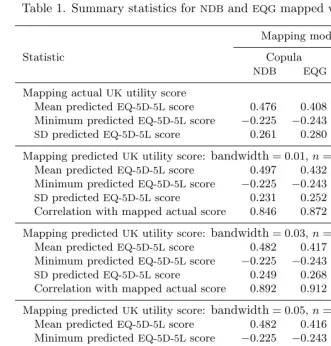
Table 1. Summary statistics for NDBandEQGmapped values for EQ-5D-5L

Mapping model based on . . .

Statistic Copula Gauss

NDB EQG NDB EQG

Mapping actualUKutility score

Mean predictedEQ-5D-5Lscore 0.476 0.408 0.461 0.400 Minimum predictedEQ-5D-5Lscore −0.225 −0.243 −0.218 −0.239

SDpredictedEQ-5D-5Lscore 0.261 0.280 0.257 0.265

Mapping predictedUKutility score: bandwidth= 0.01,n= 38590

SDpredictedEQ-5D-5Lscore 0.231 0.252 0.228 0.239 Correlation with mapped actual score 0.846 0.872 0.858 0.895

Using the smallest bandwidth, 0.01,eq5dmapgives a warning. For 7% of the

obser-vations, matches could not be found within the bandwidth, generating missing mapped

values. These observations tend to be at the extremes of the EQ-5D-3L distribution,

where the gaps between consecutive utility values are substantial.8 _{Even this small}

number of missing values is enough to distort the mean because missingness is not sym-metric across the upper and lower tails of the utility distribution. For that reason, it is usually unwise to use a very small bandwidth when utility values are approximate. In this case, a slightly larger bandwidth of 0.03 resolved the existence issue, and in our artificial example, larger bandwidths generated a result more highly correlated with the result of an exact mapping of actual scores: compare the rows of table 1 for bandwidths

(16)

0.03, 0.05, and 0.1. The mean of the predicted scores is fairly stable for different

band-widths, and, as expected, theSDdecreases as the bandwidth increases. Note that, for

any bandwidth, the mean of the mapped approximate utility is systematically above the mean of the mapping from the actual utility score. This happens to be due to the arbitrary method we used to generate hypothetical utility values; it is not inherent

in the mapping approach.9 _{Specific guidance on the bandwidth choice when mapping}

a single overall mean utility from EQ-5D-3L to EQ-5D-5L is given in Pennington et al.

(Forthcoming). Based on the two available reference datasets, it is shown that small bandwidths, no larger than 0.1 but large enough to cover the full health value of 1,

work well when the overall mean utilityE(υ3) in the trial is in the interval (1,0.7] (this

guarantees that a full health response inEQ-5D-3Lis included in the distance-weighted

average in an area where there is a large gap in theEQ-5D-3Ldistribution). If the mean

utility is in the interval (0.7,0.6], a larger bandwidth of 0.2 is preferred; for mean

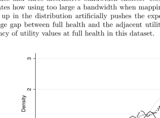
utili-ties below 0.6, an even larger bandwidth of about 0.4 is preferable. Figure 1 compares

the kernel densities of the mapped values using exact matching of the EQ-5D-3L

util-ity values and three alternative bandwidth choices: 0.03, 0.10, and 0.20. The figure illustrates how using too large a bandwidth when mapping from utility scores that are higher up in the distribution artificially pushes the expected values down because of the large gap between full health and the adjacent utility value and the relative high frequency of utility values at full health in this dataset.

0

1

2

3

Density

−.5 0 .5 1

bwidth=0.001 bwidth=0.03

bwidth=0.10 bwidth=0.20

kernel = epanechnikov, bandwidth = 0.0280

Figure 1. Kernel densities of mapped values for EQ-5D-5L using the copula mixture

model and the NDB reference dataset; exact matching of individual EQ-5D-3L utility

values versus approximate utility values for alternative bandwidths

[image:16.612.105.382.310.514.2]

(17)

The second important issue that should be considered in choosing a bandwidth

for mapping from an approximate utility score υb3 is monotonicity. If a trial

estab-lishes that procedure 1 gives a better expected EQ-5D-3L outcome than procedure 2,

there will be serious difficulty in implementing cost-effectiveness analysis if the mapped

EQ-5D-5L measure reverses that ranking, purely because of the choice of bandwidth.10

Perverse outcomes of this type can be avoided if the mapping functionυb5(υb3)

gener-ated by eq5dmap is monotonically increasing. The relationship between monotonicity

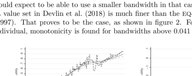
and bandwidth choice can be illustrated by applying eq5dmap over a grid of values

b

υ3 =−0.594, . . . ,1.0 for alternative bandwidths; figure 2 plots the 3L →5L mapping

function for alternative bandwidths, using theNDB copula-mixture model applied to a

hypothetical 40-year-old male. In this case, the function is monotonic only for

band-widths of 0.207 or larger; if we switch to the same model based on the EQG reference

dataset, monotonicity applies for bandwidths above 0.190.

The same procedure can be used to examine monotonicity of 5L→3L mapping. We

would expect to be able to use a smaller bandwidth in that case because theUK

EQ-5D-5Lvalue set in Devlin et al. (2018) is much finer than theEQ-5D-3L value set in Dolan

(1997). That proves to be the case, as shown in figure 2. For the same hypothetical

individual, monotonicity is found for bandwidths above 0.041 (NDB) or 0.060 (EQG).

[image:17.612.79.408.292.422.2]

(a) 3L→5L (b) 5L→3L

Figure 2. The effect of bandwidth choice on monotonicity of mapping functions

(copula-mixture model;NDBreference data; 40-year-old male)

Although users of eq5dmap will want to investigate the sensitivity of results to

al-ternative choices of bandwidth, we would strongly advise caution with mapping from an approximate utility score—it should be avoided in favor of exact individual-level mapping if at all possible; and, where unavoidable, it should not be done using

band-widths substantially less than 0.2 for 3L→5L mapping or 0.05 for 5L→3L mapping if

monotonicity is required. As discussed above, exceptions to this rule of thumb should be made if the trial subjects are believed to be concentrated at either extreme of the health distribution. We recommend that sensitivity analysis always be carried out and reported.

10. Nonmonotonicity is also a possibility in exactY3→υ5mapping, and the possibility is inherent in

(18)

5.4 Sensitivity of mapping outcomes to the choice of reference

data-set

A reference dataset is one that contains simultaneous observations on the two versions of

EQ-5D. From that dataset, our estimate of the joint distribution ofEQ-5D-3Land

EQ-5D-5Lresponses is derived, which in turn is used to form a conditional predictor ofEQ-5D-5L.

Different reference datasets will yield different mapping results, and it is important to know how great those differences might be to give some indication of robustness. We

compare results based on theNDBdataset, which covers North American patients with

rheumatoid arthritis, with results based on EQG, which is an assemblage of ad hoc

samples collected in several European countries. Do these very different samples give a similar picture of the relationship between responses to the three-level and five-level

versions ofEQ-5D? We also investigate the effects of model choice by comparing mapping

results from the copula-mixture and Gaussian specifications.

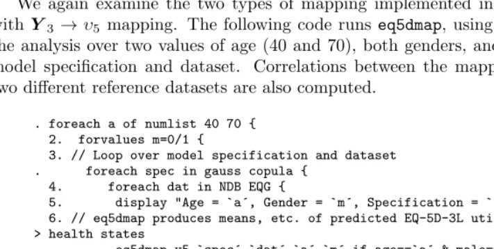
We again examine the two types of mapping implemented in eq5dmap, beginning

withY3 →υ5 mapping. The following code runseq5dmap, using four loops to repeat

the analysis over two values of age (40 and 70), both genders, and the two choices for model specification and dataset. Correlations between the mapped results using the two different reference datasets are also computed.

. foreach a of numlist 40 70 { 2. forvalues m=0/1 {

3. // Loop over model specification and dataset . foreach spec in gauss copula {

4. foreach dat in NDB EQG {

5. display "Age = `a´, Gender = `m´, Specification = `spec´, Data = `dat´" 6. // eq5dmap produces means, etc. of predicted EQ-5D-3L utility scores across > health states

. eq5dmap v5_`spec´_`dat´_`a´_`m´ if age==`a´ & male==`m´, > covariates(age male) model(`dat´`spec´)

> items(Y3_1 Y3_2 Y3_3 Y3_4 Y3_5)

7. }

8. }

9. // Compute correlations between results for different reference datasets . correlate v5_gauss_NDB_à´_`m´ v5_gauss_EQG_à´_`m´ if age==à´ & male==`m´

10. correlate v5_copula_NDB_à´_`m´ v5_copula_EQG_à´_`m´ if age==à´ & male==`m´ 11. }

12. }

[image:18.612.75.431.296.475.2]

(output omitted)

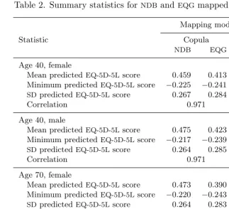
Table 2 summarizes the results in terms of the mean score, minimum score, andSD

across EQ-5D-5L health states, together with the correlations between predictions

pro-duced by each model specification on the two reference datasets. The mean prediction is

always larger using the NDBrather than theEQGdataset and the mixed copula rather

(19)

[image:19.612.81.404.85.379.2]

Table 2. Summary statistics for NDBandEQGmapped values for EQ-5D-5L

Mapping model based on . . .

Statistic Copula Gauss

NDB EQG NDB EQG

Age 40, female

Correlation 0.971 0.980

Age 40, male

Age 70, female

Age 70, male

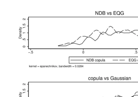
Figure 3 plots the empirical distributions (kernel densities) of the mappedEQ-5D-5L

values for a 70-year-old male. For a given choice of model (the copula-mixture model is illustrated), there are noticeable differences between the results for the two reference

datasets. For a given reference dataset (theNDB is illustrated), the difference between

(20)

0

.5

1

1.5

2

Density

−.5 0 .5 1

NDB copula EQG copula

NDB vs EQG

0

.5

1

1.5

2

Density

−.5 0 .5 1

NDB copula NDB gauss

[image:20.612.124.365.66.234.2]

copula vs Gaussian

Figure 3. Comparison of kernel densities of mapped values forEQ-5D-5Lfor a 70-year-old

male

Next, we repeat the exercise for aυ3→υ5 mapping using the entire dataset. First,

we use u3, the variable containing the actual UK utility scores corresponding to the

health states described by the variables Y3 1 to Y3 5. The following code produces

results that are summarized in the first section of table 1.

. // Actual UK 3-level utility scores:

. // loop over model specification and dataset . foreach spec in gauss copula {

2. foreach dat in NDB EQG {

3. display "Specification = `spec´, Data = `dat´" 4. display "Actual UK scores..."

5. eq5dmap v5_`spec´_`dat´_actual,

> covariates(age male) model(`dat´`spec´) > score(u3) bwidth(0.001)

6. } 7. }

(output omitted)

As before, all mappings using theNDBdataset produce higher-average mapped values

than those using theEQG dataset (see table 1). The smaller the bandwidth, the lower

the correlations with the values mapped from the actual utility scores and also the

smaller the SDs of the mapped values.

5.5 Mapping using weights

Our dataset contains a row for every possibleEQ-5D-3Lhealth state by age and gender.

(21)

proportion of health states in the three-level descriptive system with associated utility scores around and below 0 (equivalent to death). Even disease-specific samples in very severely affected subpopulations usually have much larger average three-level utility

scores: for example, the mean three-level utility values in the EQG and NDB samples

are 0.628 and 0.681, respectively, and the proportion of individuals with a negative utility value is only 8% and 4%. This contrasts with the almost 35% health states with negative utility values in the whole 3L descriptive system.

In this section, we demonstrate the use of the weighting option to calculate the

mean mapped five-level utility for the populations in the EQG and the NDB samples.

The variablesfwEQGandfwNDBin the dataset contain frequency weights describing the

demographic composition of the EQG and NDB data, respectively. The following code

continues with the choice of theNDBmixed copula mapping model to map theEQ-5D-3L

descriptive items into a predicted five-level utility score, but it uses theEQG frequency

weights to calculate the weighted mean of the mapped utility score.

. eq5dmap v5_y3EQG [fw = fwEQG], covariates(age male) model(NDBcopula) > items(Y3_1 Y3_2 Y3_3 Y3_4 Y3_5)

Weighted mean of predicted 5L score within selected sample

v5_y3EQG 3,539 .7088379 .2298323 -.2170747 .9587727

Now, we carry out the same mapping but using theNDBfrequency weights instead.

. eq5dmap v5_y3NDB [fw = fwNDB], covariates(age male) model(NDBcopula) > items(Y3_1 Y3_2 Y3_3 Y3_4 Y3_5)

Weighted mean of predicted 5L score within selected sample

v5_y3NDB 5,205 .7640676 .1689144 -.2246118 .9584147

The mean difference between three-level and five-level utility scores calculated for

theEQG andNDBsample compositions are fairly small—0.081 and 0.083, respectively.

In comparison, the average three-level or five-level difference is 0.339 when calculated

(22)

age-gender groups. This is consistent with the findings in Hern´andez-Alava and Pudney (2017) and Hern´andez-Alava et al. (2018) of minor differences between three-level and

five-levelEQ-5Dat the top of their range but much larger differences at the bottom.

We now investigate the effect of using alternative weights on the correlations between the mappings based on different reference datasets. The following code calculates the

correlations between the υ3→υ5 mapped values in section 5.4 using the mixed copula

model.

. // calculate correlations - unweighted

. correlate v5_copula_NDB_actual v5_copula_EQG_actual (obs=41,310)

v5_cop.. v5_cop..

v5_copula_.. 1.0000

v5_copula_.. 0.9549 1.0000

. // calculate correlations - weighted

. correlate v5_copula_NDB_actual v5_copula_EQG_actual [fw = fwNDB] (obs=5,205)

v5_cop.. v5_cop..

v5_copula_.. 1.0000

v5_copula_.. 0.9967 1.0000

. correlate v5_copula_NDB_actual v5_copula_EQG_actual [fw = fwEQG] (obs=3,539)

v5_cop.. v5_cop..

v5_copula_.. 1.0000

v5_copula_.. 0.9959 1.0000

The unweighted correlation between the mapped values using different reference

datasets is high (0.9549) when calculated unweighted across all possible EQ-5D-3L

out-comes, and it increases to a value close to 1 when the sample is weighted to either

the NDBor the EQG composition. This serves to demonstrate that inconsistencies

be-tween EQ-5D-3L and EQ-5D-5L utility scores are moderate in samples with a realistic

composition and that their main feature is difference in the mean rather than lack of correlation.

6 Conclusion

In this article, we presented a new command, eq5dmap, that calculates the

predic-tion of EQ-5D-3L utility scores from observed or specified values of EQ-5D-5L

(indi-vidual items or utility score), age and gender, and vice versa. The predictive

dis-tribution was derived from a joint model of the two versions of EQ-5D developed in

(23)

7 Acknowledgments

This work was supported by the National Institute for Health and Care Excellence with its Decision Support Unit and the Medical Research Council (grant MR/L022575/1).

Pudney acknowledges furtherESRCfunding through the Centre for Micro-Social Change

(grant RES-518-28-5001). The views expressed in this article, and any errors or omis-sions, are those of the authors only.

We thank Kaleb Michaud (University of Nebraska Medical Center and National Data Bank for Rheumatic Diseases), Frederick Wolfe (National Data Bank for Rheumatic Diseases), and the EuroQol Group for providing the data used in the calculation of the weighting variables in section 5.

8 References

Augustovski, F., L. Rey-Ares, V. Irazola, O. U. Garay, O. Gianneo, G. Fern´andez,

M. Morales, L. Gibbons, and J. M. Ramos-Go˜ni. 2016. AnEQ-5D-5L value set based

on Uruguayan population preferences. Quality of Life Research25: 323–333.

Devlin, N., K. Shah, Y. Feng, B. Mulhern, and B. van Hout. 2016. Valuing

health-related quality of life: AnEQ-5D-5Lvalue set for England. Office of Health Economics,

London, UK.

Devlin, N. J., K. K. Shah, Y. Feng, B. Mulhern, and B. van Hout. 2018. Valuing

health-related quality of life: An EQ-5D-5L value set for England. Health Economics

27: 7–22.

Dolan, P. 1997. Modeling valuations for EuroQol health states. Medical Care35: 1095–

1108.

Hern´andez-Alava, M., and S. Pudney. 2017. Econometric modelling of multiple

self-reports of health states: The switch from EQ-5D-3L to EQ-5D-5L in evaluating drug

therapies for rheumatoid arthritis. Journal of Health Economics 55: 139–152.

Hern´andez-Alava, M., A. Wailoo, S. Grimm, S. Pudney, M. Gomes, Z. Sadique,

D. Meads, J. O’Dwyer, G. Barton, and L. Irvine. 2018. EQ-5D-5L versus EQ-5D-3L:

The impact on cost effectiveness in the United Kingdom. Value in Health21: 49–56.

Hern´andez Alava, M., A. J. Wailoo, and R. Ara. 2012. Tails from the peak district:

Adjusted limited dependent variable mixture models of EQ-5D questionnaire health

state utility values. Value in Health15: 550–561.

van Hout, B., M. F. Janssen, Y.-S. Feng, T. Kohlmann, J. Busschbach, D. Golicki, A. Lloyd, L. Scalone, P. Kind, and A. S. Pickard. 2012. Interim scoring for the

EQ-5D-5L: Mapping theEQ-5D-5LtoEQ-5D-3Lvalue sets.Value in Health15: 708–715.

Janssen, M. F., A. S. Pickard, D. Golicki, C. Gudex, M. Niewada, L. Scalone, P.

(24)

to the EQ-5D-3L across eight patient groups: A multi-country study. Quality of Life Research22: 1717–1727.

Kim, S.-H., J. Ahn, M. Ock, S. Shin, J. Park, N. Luo, and M.-W. Jo. 2016. TheEQ-5D-5L

valuation study in Korea. Quality of Life Research25: 1845–1852.

Luo, N., G. Liu, M. Li, H. Guan, X. Jin, and K. Rand-Hendriksen. 2017. Estimating anEQ-5D-5Lvalue set for China. Value in Health 20: 662–669.

NICE. 2014. DevelopingNICEguidelines: The manual. National Institute for Health and

Care Excellence. https: // www.nice.org.uk / process / pmg20 / chapter / introduction-and-overview#updating-this-manual.

Pennington, B., M. Hern´andez-Alava, S. Pudney, and A. J. Wailoo. Forthcoming.

Com-paring theEQ-5D-3Land5Lversions. What are the implications for model-based cost

effectiveness estimates? Decision Support Unit report.

Purba, F. D., J. A. M. Hunfeld, A. Iskandarsyah, T. S. Fitriana, S. S. Sadarjoen, J. M.

Ramos-Go˜ni, J. Passchier, and J. J. V. Busschbach. 2017. The IndonesianEQ-5D-5L

value set. PharmacoEconomics 35: 1153–1165.

Shiroiwa, T., S. Ikeda, S. Noto, A. Igarashi, T. Fukuda, S. Saito, and K. Shimozuma.

2016. Comparison of value set based onDCEand/orTTOdata: Scoring forEQ-5D-5L

health states in Japan. Value in Health 19: 648–654.

Versteegh, M. M., K. M. Vermeulen, S. M. A. A. Evers, G. Ardine de Wit, R. Prenger,

and E. A. Stolk. 2016. Dutch tariff for the five-level version ofEQ-5D.Value in Health

19: 343–352.

Wolfe, F., and K. Michaud. 2011. The National Data Bank for rheumatic diseases: A

multi-registry rheumatic disease data bank. Rheumatology 50: 16–24.

Xie, F., E. Pullenayegum, K. Gaebel, N. Bansback, S. Bryan, A. Ohinmaa, L. Poissant,

and J. A. Johnson. 2016. A time trade-off-derived value set of the EQ-5D-5L for

Canada. Medical Care 54: 98–105.

About the authors

M´onica Hern´andez-Alava is an applied microeconometrician in the Health Economics and De-cision Science section in ScHARR, University of Sheffield,UK.