A Modified Replacement Model for Items That Fail Suddenly with Variable Replacement Costs

(1)

ISSN Online: 2160-8849 ISSN Print: 2160-8830

DOI: 10.4236/ajor.2018.86026 Nov. 5, 2018 457 American Journal of Operations Research

A Modified Replacement Model for Items

That Fail Suddenly with Variable

Replacement Costs

Samuel Ugochukwu Enogwe

1*

, Ben Ifeanyichukwu Oruh

2

, Emmanuel John Ekpenyong

2

1_{Department of Mathematics/Statistics, Federal Polytechnic Nekede, Owerri, Imo State, Nigeria} 2_{Department of Statistics, Michael Okpara University of Agriculture, Umudike, Abia State, Nigeria}

Abstract

Several researches have been done to provide better alternative to the existing replacement models, but the research works did not adequately address the replacement problem for items that fail suddenly. Hence, a modified re-placement model for items that fail suddenly has been proposed using the knowledge of probability distribution of failure times as well as that of varia-ble replacement cost. The modified cost functions for implementing both in-dividual and group replacements were derived. The modified cost functions were minimized using the principle of classical optimization in order to find the age at which replacement of items would be appropriate. Conditions un-der which the individual and group replacement policies should be adopted were derived. Two real data sets on failure time of LED bulbs and their re-placement costs were used to validate the theoretical claims of this work. In essence, goodness-of-fit test was used to select appropriate probability distri-bution of failure times as well as that of replacement costs for data sets I and II respectively. The goodness-of-fit results showed that failure times of LED bulbs follow the Smallest Extreme Value and Laplace distributions for data sets I and II respectively. Similarly, it was observed that individual replace-ment cost followed the two-parameter Gamma and Largest Extreme Value distributions for data sets I and II respectively. Further, the group replace-ment cost was found to follow the log-normal and two-parameter Weibull distributions for data sets I and II respectively. Based on the empirical study, we observed that individual replacement policy is better than group replace-ment policy in terms of cost minimization for both existing model and the proposed model. In view of the results, the proposed replacement policy was recommended over the existing one because it yielded lower replacement costs than the existing replacement model.

How to cite this paper: Enogwe, S.U., Oruh, B.I. and Ekpenyong, E.J. (2018) A Modified Replacement Model for Items That Fail Suddenly with Variable Replace-ment Costs. American Journal of Operations Research, 8, 457-473.

https://doi.org/10.4236/ajor.2018.86026

Received: August 25, 2018 Accepted: November 2, 2018 Published: November 5, 2018

http://creativecommons.org/licenses/by/4.0/

(2)

DOI: 10.4236/ajor.2018.86026 458 American Journal of Operations Research

Keywords

Probability Distribution, Failure Times, Variable Replacement Cost, Goodness-of-Fit Test, Group Replacement, Individual Replacement

1. Introduction

In many organizations, several job performing units like men, machines, equip-ment, parts etc. are used for carrying out day-to-day activities. When any job performing unit is new, it works with full operating efficiency and due to usage or of time, it may become old and some of its components wear out and the op-erating efficiency of the job performing unit falls down. In order to regain the ef-ficiency, maintenance is carried out. The act of maintenance consists of replac-ing the worn out part, or oilreplac-ing or overhaulreplac-ing, or repair etc. Once maintenance is attended, the efficiency may not be regained to the previous level but a bit less than that of the previous level. For example, if the operating efficiency is 95 per cent and due to deterioration, the efficiency reduces to the level of 90 per cent, after maintenance, it may regain to the level of 93 percent. Once again due to usage, the efficiency falls down and the maintenance is to be attended. After some time, the efficiency reduces to such a level that the maintenance cost will become very high and due to low efficiency, the unit production cost will be very high and at this time, the management has to think of replacing the job per-forming unit. According to [1], the replacement problem arises because of three factors: 1) the existing unit may have outlived its effective life and it may not be economical to allow it to continue in the organization, 2) the existing unit may have been destroyed through accident or otherwise and, 3) the present unit might have become obsolete because of new discoveries and better design of the equipment.

(3)

The ultimate objective of this paper is to propose an improved model for op-timal replacement of items that fail suddenly by putting forward a replacement model that will modify [7] replacement model based on the assumption that the cost of replacement is a random variable which must be governed by some probability laws. Thus, we will propose a cost function that accommodates re-placement cost as a random variable and then utilize goodness-of-fit test to de-termine the probability distribution for replacement cost as well as for failure times.

2. Review of Replacement Model for Items That Fail

Suddenly Where Cost Is Assumed Fixed

2.1. The Existing Cost Function for Individual Replacements

The average cost of individual replacement, A( )in is given in [7] as:

( )in

_{( )}

i N

A C

E X

= ₍₁₎

where Ci is the cost per item for individual replacement, E X

( )

is the

ex-pected life of the item, and N is the total number of items in the system. The expression for computing E(X) of Equation (1) is given as:

( )

1 K

j j

E X jP

=

∑

₍₂₎

where Pj is the probability of items that fail at the end of jth period and k is the

end of the period of each replacement. Works by [1], [7], [8], [9] used mortality tables to derive the probability distribution of failures of the items in the system. According to them, the probability that any item will fail in the interval (t − 1, t) is given as:

( )t1 ( )t x

M M

P

N − −

= _, M_{( )}_t−₁ >M_{( )}_t (3)

where M( )t−1 is the number of survivors at any time, t − 1, M( )t is the number

of survivors at time, t and N is the initial number of items in the system. The in-dividual replacement policy is concerned with replacing an item as at when it fails and Equation (1) is the average individual replacement cost per period.

2.2. The Existing Cost Function for Group Replacements

The average cost of group replacement per period A( )gn is given in [7] as:

( ) ( )

( )

1

1 n g i n

g X

n

NC C N X

C A

n n

−

=

+

= =

∑

₍₄₎

where C( )n is the total cost of group replacement, N X

( )

is the number of

failures (or replacements) at the end of the jth period, Ci is the cost per item

for individual replacement, Cg is the cost of replacing an item when all the

(4)

The expression for computing N X

( )

of Equation (4) is as given below

( )

1 , 1,2, , X

X j j j

N X N P X− n

=

∑

= _ ₍₅₎

3. The Proposed Replacement Model for Items That Fail

Suddenly Where Cost Is Assumed to Be a Random

Variable

3.1. The Proposed Cost Function for Individual Replacement of

Items That Fail Suddenly

In Equation (1) and Equation (4) respectively, [7] assumed that Ci and Cg are

fixed (or constant) over time. However, in reality, rarely do costs of replacement of items appear to be fixed over time due to the dynamic nature of the world’s economy. Since the values of Ci and Cg cannot be predicted with certainty, it

suf-fices to view Ci and Cg as random variables that can be governed by some

proba-bility laws. Based on the probaproba-bility distributions of Ci and Cg respectively, we

now obtain the expected values E(Ci) and E(Cg) [10]. Thus, the cost function due

to [7] would be modified to include replacement costs that are random in na-ture. Thus, the cost of replacing an individual item on its failure is proposed to be:

m i

i V

C =C ₍₆₎

where m

i

C is the modified cost of replacing an individual item on failure i V C

is the variable cost of replacing an individual item on its failure.

Substituting Equation (6) into Equation (1), we obtain the modified cost func-tion for individual replacement of items that fail suddenly as:

( )i

_{( )}

i

mAn =_{E X}N CV (7)

where mA( )in is the modified average cost of individual replacement per period.

Since variable cost component, i V

C has been incorporated into the replace-ment function in Equation (1), it is worthwhile to determine a probability dis-tribution for i

V

C so that the expected value of i V

C is

( )

i V

E C . If we take the expectation of both sides of Equation (7), we obtain

( )i

_{( )}

( )

i

m n N V

E A E C

E X

 _{ =}

  (8)

3.2. The Proposed Cost Function for Group Replacement of Items

That Fail Suddenly

Let C( )mn be the modified cost of replacing items as a group, CVi is the variable

cost of replacing an individual item on its failure and g V

C is the variable cost per item when all items are replaced as a group. Then substituting i

V

C for and

g V

(5)

DOI: 10.4236/ajor.2018.86026 461 American Journal of Operations Research ( ) ( )

( )

1 1 n g i

m _V _V

n

g X

m n

NC C N X

C A n n − = +

= =

∑

₍₉₎

Taking expectation of both sides of Equation (9), we obtain;

( ) ( )

1

( )

1 n

g i

m _V _V

n

g X

m n

NE C E C N X

E C E A n n − = +      _{ =} =  

∑

(10)

We shall obtain the value of n that minimizes Equation (10) using classical optimization.

3.3. Determination of Optimal Replacement Policy for Items That

Fail Suddenly

Recall from the numerator of Equation (4.9) that,

( )

( ) ( )

( )

1

n

m g i

V V

n

X

E C NE C E C − N X

=

  = +

 

∑

(11)

If we replace n by n + 1 in Equation (4.10), we obtain

( )

( ) ( )

( )

( ) ( )

( )

(

)

( )

( ) ( )

( )

( ) ( )

( )

1 1 1 1 1 1 1 1 1

1 2 1

n

m g i

V V

n

X

m g i

V V

n

m g i

V V

n

X n

m g i i

V V V

n

X

E C NE C E C N X

E C NE C E C N N N n N n

E C NE C E C N X N n

E C NE C E C N X E C N n

+ = + − + = − + =  _{ =} ₊    _{ =} + _ + + + − + _      _{ =} ₊ _ ₊ _   _ _  _{ =} + +  

∑



( )mn1 ( )mn

( )

Vi

( )

E C + =E C +E C N n (12)

If we replace n by n − 1 in Equation (11), we obtain;

( )

( ) ( )

( )

( ) ( )

( )

(

)

2 1

1

1 1 2 2

n

m g i

V V

n

X

m g i

V V

n

E C NE C E C N X

E C NE C E C N N N n

− − = −  _{ =} +    _{ =} ₊ __ ₊ _{+ +} ₋ __  

∑

 ( )

( ) ( )

( )

(

)

(

)

(

)

1 1 2 2

1 1

m g i

V V

n

E C NE C E C N N N n

N n N n

−  _{ =} + _ + + + −   + − − _{− }  ( )

( ) ( )

( )

(

)

1 1 1 1 n

m g i

V V

n

X

E C − NE C E C − N X N n

=    _{ =} + _ − − _   _

∑

_ ( )

( ) ( )

( )

(

)

1 1 1 1 n

m g i i

V V V

n

X

E C − NE C E C − N X E C N n

=

  = + − −

 

∑

( )mn1 ( )mn

( )

Vi

(

1

)

E C − =E C −E C N n− (13)

( )mn ( )mn1

( )

Vi

(

1

)

E C  E C −  E C N n

⇒ _ _= _ _+ − ₍₁₄₎

From Equation (10), we define

( ) ( ) 1 1 ₁ m n g m n E C E A n + +       =

(6)

Substituting Equation (14) into Equation (15), we obtain

( ) ( )

( )

1 ₁ m i V n g m n

E C E C N n

E A n +   +     =

  ₊ (16)

From Equation (10), we define

( ) ( ) 1 1 ₁ m n g m n E C E A n − −       =

  ₋ (17)

( ) ( )

( )

(

)

1 1 1 m i V n g m n

E C E C N n

E A n −   − −     =

  ₋ (18)

and from definition, we know that

( )g ( )g 1 ( )g

m n m n m n

E A  E A +  E A 

∆ _ _= _ _− _ _₍₁₉₎

Substituting Equation (10) and Equation (16) into Equation (19), we obtain

( ) ( )

( )

( ) ( ) ( )

( )

( ) (

)

( )

(

)

( ) ( )

( )

( ) ( )

(

)

( )

(

)

( )

( ) 1 1 1 1 1

m i m

V

n n

g m n

m i m

V

n n

g m n

m i m m

V

n n n

g m n i m V n g m n m n i V g m n

E C E C N n E C

E A

n n

nE C nE C N n n E C

E A

n n

nE C nE C N n nE C E C

E A

n n

nE C N n E C

E A

n n

E C n E C N n

n E A  +         ∆ _ _= − +  ₊ ₋ ₊         ∆ _ _= +  + −  −           ∆ _ _= +   −     ∆ _ _= +     ₋        ∆ _ _=

(

1

)

n n   + ( )

( )

(

1

)

m n i V g m n E C E C N n

n E A n     −   ∆ _ _=

+ (20)

From definition, we know that

( )g 1 ( )g ( )g 1

m n m n m n

E A −  E A  E A − 

∆ _ _= _ _− _ _₍₂₁₎

Substituting Equation (10) and Equation (17) into Equation (21), we obtain

( ) ( )

{

( )

(

)

}

( )

(

)

( )

{

( )

(

)

}

(

)

( ) ( ) ( ) ( )

( )

(

)

(

)

1 1 1 1 1 1 1 1 1 1 m i m V n n g m n

m m i

V

n n

g m n

m m m i

V

n n n

g m n

E C E C N n

E C

E A

n n

n E C n E C E C N n

E A

n n

nE C E C nE C n E C N n

(7)

DOI: 10.4236/ajor.2018.86026 463 American Journal of Operations Research ( )

( )

(

)

( )

(

)

1 1 1 i m V n g m n

n E C N n E C

E A n n −     − −       ∆ _ _=

− (22)

( )

(

)

( )

(

)

(

)

( )

(

)

( )

(

)

( )

(

)

( )

(

)

( )

(

)

( )

(

)

( )

(

)

( )

(

)

( )

(

)

1 1 1 1 1 1 1 1 1 1 1 1 1 1 1 1 1 1 1 1 1

i m i

V n V

g m n

i i m

V V n

g m n i m V n g m n m n i V g m n

nE C N n E C E C N n

E A

n n

nE C N n E C N n E C

E A

n n

n E C N n E C

E A

n n

E C

n E C N n

n E A n n − − − − − − − −   − − _ _+ −   ∆ _ _= −   − − _{− − } _   ∆ _ _= −   − _{− − } _   ∆ _ _= −       −  − − ₋        ∆ _ _= − ( )

( )

(

)

( )1

1 1 1 m n i V g m n E C E C N n

n E A n − −     − − −  

∆ _ _= ₍₂₃₎

Thus, according to [11], E A ( )n is minimum if and only if:

( )n1 0 ( )n E A −  E A 

∆ _ _< < ∆ _ _₍₂₄₎

The condition stated in Equation (24) stem from the fact that the function,

( )n E A 

  is said to be achieve its minimum value at a point, n, if

( )n1 0

E A − 

∆ _ _< _or ∆E A _{( )}n >0

where ∆E A ( )n−1=E A ( )n −E A ( )n−1 and ∆E A ( )n=E A ( )n+1−E A ( )n .

From Equation (24), the condition ∆EmA( )gn−1<0 gives

( )

(

)

( )

(

)

( ) 1 1 1 1 ₀ 1 0 1 m n i V m n i V E C

E C N n

n n

E C

E C N n

n − −       − −   ₋ <    

  − − <

  ₋

( )

(

)

( )1

1 1 m n i V E C

E C N n

n

−

 

 

  − <

  ₋ (25)

Equation (25) states that group replacement should not be made at the end of nth period if the expectation of average cost of individual replacement at the end of (n − 1)th period is not less than the overall expectation of average cost per unit period by the end of (n − 1) periods.

(8)

( )

(

)

( )

_{( )}

( )

0

1

0

m n i

V

m n i

V m

n _i

V E C E C N n

n n

E C E C N n

n E C

E C N n n

 

 

− <

+

 

 

< −

 

 _{ <}

( )

_i

( )

( )mn

V

E C E C N n

n

 

 

⇒ > (26)

Equation (26) states that group replacement should be made at the end of nth period if the expectation of average cost of individual replacement for the nth period is greater than the overall expectation of average cost per unit time period through the end of n periods.

4. Numerical Illustrations

In this section we shall make use of real-life data collected from two different hotels to validate the theoretical results of this work and the results are presented in Table 1. Prior to computing the necessary estimates of the replacement mod-els, we shall first fit the probability distributions of failure times and those of re-placement costs.

4.1. Fitting Probability Distribution of Failure Times

In order to apply Equation (5), we need to estimate the probability of failure times, Pj. In this regard, we cannot just employ any kind of probability

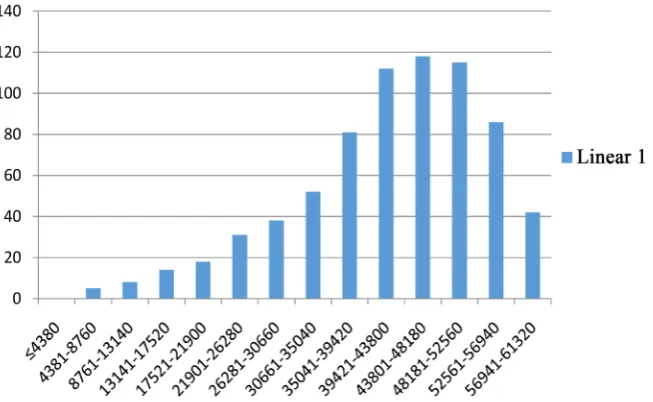
distribu-tion by mere guesses. According to [12], a number of probability distribution may be used to model the life time of items. Thus, to determine the appropriate probability distribution for sudden failure times, the first step is to obtain the histogram of the failure time data and then visually inspect the pattern of the graph. On the basis of the pattern of the histogram, we can suggest theoretical distribution(s) for the failure time data under consideration. The next challenge now lies on determining whether or not the distributions that have been sug-gested actually fit the failure time data. To achieve this purpose, we shall utilize the goodness-of-fit test.

(9)

[image:9.595.62.539.89.486.2]

Table 1. Results of the empirical analysis based on existing and proposed replacement models.

Results Existing Method [7] Proposed Method

Data Sets Data Set I Data Set II Data Set I Data Set II

Fitted Probability

Distribution for failure times … …

Smallest Extreme Value (or Gumbel) with:

34.25888 34.11878

µ σ = =

Laplace with:

5183.0120 94.2625

θ φ = =

Fitted Distribution for

|Individual Replacement Cost … …

Gamma with:

13.68094 42.42969

α β = =

Largest Extreme Value with: 501.57496 55.02559

µ σ = =

Fitted Distribution for

Group Replacement Cost … …

Lognormal with: 5.76867 0.16455

µ σ = =

Weibull with:

159.14436 1.68840

α β = =

Expected Cost of Replacement

i

C = N 700.00

g

C = N 400.00

i

C = N 700.00

g

C = N 400.00

( )

i V

E C = N 580.38

( )

g V

E C = N 324.47

( )

i 533.34

V

E C =

( )

g 354.76

V

E C =

Average Cost of Individual

Repl. Policy per period A( )in = N55,300.00 A( )in = N 54,600.00 E A ( )in = N 46,427.20 E A ( )in = N 41,600.52

Average Cost of Group

Repl. Policy per period A( )gn = N 57,000.00 A( )gn = N 54,450.00 E A ( )gn = N 49,4538.00 E A ( )gn = N 50,441.00

Appropriate time to replace failed LED bulbs

After every 8th_period

(i.e., after every 39,420 burning hours)

(i.e., after every 30,660 burning hours) Expected Life

of an LED bulb 9.1109 hours 7.5307 hours 9.03971 hours 7.53074 hours Average No. of

replaced bulbs 79 bulbs 78 bulbs 80 bulbs 78 bulbs

Average cost of individual

replacement per hour N 12.63 N 12.47 N 10.60 N 9.50

grouping of the data or determination of intervals. One of the major limitations of Kolmogorov-Smirnov (K-S) test is that it does not detect the discrepancies at tails very well; however the Anderson-Darling (AD) test is mainly designed to detect the discrepancies in tails [13], [14], [15]. In the same vein, [12] recom-mend the use of Anderson-Darling (AD) test because it is less likely to reject the good fit, and can be successfully used to compare the goodness of fit of several fitted distributions.

4.2. Anderson-Darling Test

(10)

distributions to see which one is best or to test whether a sample of data comes from a population with a specified distribution. The hypotheses for the Ander-son-Darling test are:

H0: The data follow a specified distribution;

H1: The data do not follow a specified distribution. (27)

The Anderson-Darling statistic (A2_{) is defined as}

(

)

( )

(

)

2

1 1

1 n _{2 1 ln} ₁

i n i

i

A n i F X F X

n + −

=

 

= − −

∑

− _ + − _₍₂₈₎

where F X

( )

i is the cumulative distribution function of the specified

distribu-tion and Xi are the ordered data.

If the p-value for the Anderson-Darling (AD) test is lower than the chosen significance level α_{, we reject the null hypothesis, H}_o_{and conclude that the} da-ta do not follow the specified distribution. Alternatively, the hypothesis regard-ing the distributional form is rejected at the chosen significance level α , if the test statistic, A2_{, is greater than the critical value obtained from a table. In}

gener-al, critical values of the Anderson-Darling test statistic depend on the specific distribution being tested.

[image:10.595.214.541.506.707.2]

In goodness-of-fit test, several probability distribution(s) may appear to fit the data well and there would be need to choose the best probability distribution for modeling the failure times. To select the best probability distribution from amongst the fitted distributions, we shall select a distribution with the largest p-value. Among extremely close p-values, we shall select a distribution that has been used previously for a similar data set [16]. If it is found by goodness-of-fit tests that none of the theoretical distribution of failure times fit the research da-ta, effort would be made to use a generalized probability distribution. The histo-grams for the data on failure times are as shown in Figure 1 and Figure 2 re-spectively.

(11)

[image:11.595.212.532.77.229.2]

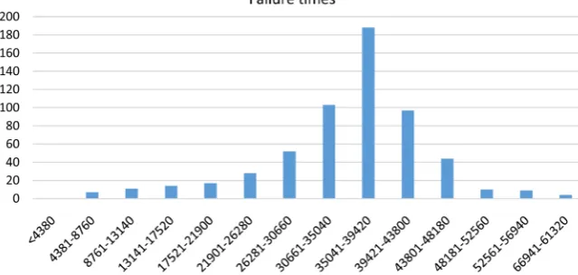
Figure 2. Histogram of LED bulb failure times for data set II.

From Figure 1, we can observe that few of the data points fall on the lower tail of the graph whereas majority of the data points fall on the upper tail of the graph. This is an indication that the failure times for data set I is skewed to the left. In Statistical theory, left skewed data can be modeled by smallest extreme value distribution or by Gumbel distribution, Lognormal, Weibull, Gamma and other kinds of skewed distributions. Having suggested some probability distri-butions for failure data set 1, it is imperative to carry out a goodness-of-fit test to determine whether or not the suggested distribution (s) fit the data well. As stated earlier, the Anderson-Darling (AD) test can be utilized for the good-ness-of-fit test. Hence, applying Equation (28) on the failure times for data set I with the aid of MINITAB software, we observe that the Smallest Extreme Value distribution best fit the data set 1 failure times for data set I.

Similarly from Figure 2, we can observe that the failure times for data set II appear to be symmetric. Theoretically, it is known that both the normal and Laplace distributions can be used to analyze symmetric data [17]. Furthermore, it is well known that the normal distribution is used to analyze symmetric data with short tails, whereas the Laplace distribution is used for symmetric data with long tails. Although, these two distributions may provide similar data fit for moderate sample sizes, however, it is still desirable to choose the correct or more nearly correct model, since the inferences often involve tail probabilities, and thus the probability density function assumption is very important [18]. To de-termine whether or not the suggested distribution(s) fit the data well, the An-derson-Darling (AD) test was utilized for the goodness-of-fit test again. Hence, applying Equation (28) on the failure times for data set II with the aid of MINITAB software, we observe that the Laplace distribution best fits the failure times for data set II.

4.3. Fitting Probability Distribution to Variable Replacement Cost

(12)

use.

Our argument in this study stems from the fact that a careful examination of the cost function due to [7] as given by Equation (1) and Equation (4) shows that individual and group replacement costs are assumed to remain the same (fixed) over time. This assumption is difficult to hold in practice because fixed costs are not permanently fixed. In other words, they will change over time but are fixed in relation to the quantity of items replaced during a particular period. For instance, an organization may have unexpected and unpredictable expenses unrelated to the replacement of items. In view of this, there are no fixed costs in the long run, because the long run is a sufficient period of time for all short-run fixed costs to become variable.

Consequently, since individual replacement cost, Ci and group replacement

cost, Cg may not remain fixed over time, it is worthwhile to view them as

ran-dom variables and then determine their respective probability distributions. Again, it is essential to choose the correct probability distribution for the cost data. [19] compared ten probability distributions viz: normal, triangular, log-normal, uniform, exponential, weibull, Beta, Rayleigh, logistic and extreme val-ue. His study revealed that beta distribution best fit the project cost data.

In line with the process taken by [19] to fit appropriate probability distribu-tion to project cost data, we shall employ the goodness-of-fit test described ear-lier in order to choose a distribution that best fit the replacement cost data prior to conducting the main numerical illustration. Once a suitable probability dis-tribution has been selected for the replacement cost data, the next task is to es-timate the expectation of individual replacement cost, E(Ci) and the expectation

of group replacement cost, E(Cg). With these expected costs, we then modify [7]

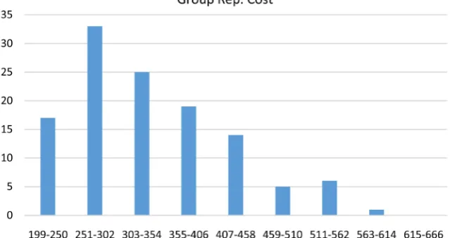
replacement cost functions accordingly. As stated in Sections 6 and 7, the histo-gram of the research data can guide us in the selection of appropriate probability distribution. Hence, the histograms for the replacement cost data are shown in

Figures 3-5.

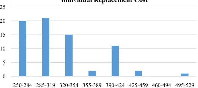
[image:12.595.213.536.561.705.2]

As Figure 3 shows, the individual replacement cost is skewed to the right. Theoretically, some of the distributions capable of characterizing right-skewed

(13)

[image:13.595.223.527.75.216.2]

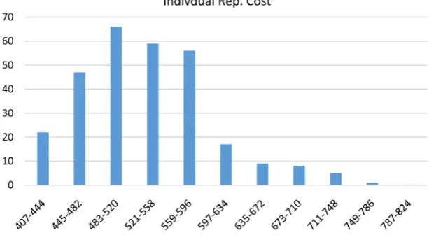
Figure 4. Histogram for group replacement cost using data set 1.

Figure 5. Histogram for individual replacement cost using data set II.

data are lognormal, Gamma, Weibull, Largest Extreme Value and many others. To determine among the aforementioned distributions, the one that best fit the data on individual replacement cost, we conducted the goodness-of-fit test and the results show that the Gamma distribution best fits the individual replace-ment cost for data set 1.

As shown in Figure 4, the group replacement cost is skewed to the right and the goodness-of-fit test is again conducted and the results show that the lognor-mal distribution provides the best fit to group replacement cost for data set 1.

As Figure 5 shows, the individual replacement cost is skewed to the right and the goodness-of-fit test shows that the Largest Extreme Value distribution fits the individual replacement cost for data set II.

Finally, as shown in Figure 6, the group replacement cost is skewed to the right and goodness-of-fit test is again conducted and the results show that the Weibull distribution approximates the group replacement cost for data set II.

5. Discussion of Results

[image:13.595.220.527.256.424.2]

(14)

[image:14.595.214.534.77.246.2]

Figure 6. Histogram for group replacement cost using data set II.

β = 42.42969. Also, results in Table 1, revealed that group replacement cost for data set I follow the lognormal distribution with location parameter, μ = 5.76867 and scale parameter, σ = 0.16455. Consequently, the average values of the indi-vidual and group replacement costs for data set I were respectively found to be N 580.34 and N 324.4 unlike that of [7] which stood at N 700 and N 400 respec-tively. This goes to show that, it is unrealistic to believe that replacement cost is fixed over time as claimed by [7]. Therefore, the proposed replacement policy has shown improvement over the existing one(s) in this regard.

Similarly, from Table 1, the individual replacement cost for data set II was found to follow the largest extreme value distribution with location parameter, μ = 501.5749 and scale parameter, σ = 55.02559. The largest extreme value distri-bution is skewed to the right. It is used to model the maximum value from a dis-tribution of random observations. Based on this disdis-tribution, it was observed that the average of the individual replacement cost is N 533.34, which is at va-riant with that of [7] that stood at N 700. Furthermore, Table 1 revealed that the group replacement cost for data set II follow a Weibull distribution with shape and scale respectively as β = 1.68840 and α = 159.14436. Consequently, the av-erage of the group replacement cost was found to be N 354.76.

(15)

re-DOI: 10.4236/ajor.2018.86026 471 American Journal of Operations Research

duced replacement cost than the existing one(s).

Also, from Table 1, when [7] replacement model was used on data set I, it was observed that individual replacement of failed bulbs is required from the first period (i.e., between 4381 and 8760 hours) through the 8th_{period (i.e., between}

35,041 - 39,420 hours) but immediately after the 8th_{period (i.e., after every}

39,420 burning hours), a group replacement is required and the average cost of group replacement would stand at about N 57,000.00. In a similar fashion, Table 1 shows that for data set I, individual replacement of failed bulbs is required from period 1 (i.e., between 4381 and 8760 hours) through period 7 (i.e., be-tween 30,661 and 35,040 hours) and immediately after the 7th_{period (i.e., after}

every 35,040 burning hours), a group replacement is required with an average group replacement cost of N 49,458.00. Here, the period of replacement ob-tained using the replacement model by [7] is at variant with that obtained using the proposed replacement model by one (1) period difference and it is evident that the proposed replacement model yields a lower group replacement cost than the existing replacement model. In comparison, it is clear that individual re-placement costs using the rere-placement model by [7] and the proposed replace-ment model on data set I, appears to be least compared to the group replacereplace-ment costs. This indicates that individual replacement cost should be adopted by Bil-ton Continental Hotels, from where data set I were collected.

From Table 1, when the replacement model by [8] was used on data set II, it was observed that, on the average a bulb would burn for about 7.53 hours. This implies that about 78 bulbs would fail per hour, resulting to average replacement cost of about N 54,600.00 per period of replacement or N 12.47 per hour. More so, the results in Table 1 revealed that when the proposed replacement model was used on data set II, then a bulb is expected to burn for about 7.53 hours, in which case about 78 bulbs would on the average die per hour. Thus, the death of these bulbs would result to about N 41,600.52 per period of replacement or N 9.50 per hour. Consequently, it is worthwhile to state that the proposed model has again showed improvement over the existing model in the area of cost re-duction.

(16)

6. Conclusions

This work discusses the construction of replacement model for items that fail suddenly. The ultimate objective is to propose a replacement model which may be used to improve the existing replacement models. In this paper, a modified replacement model for items that fail suddenly was proposed following [7]. In the proposed replacement model, individual and group replacement costs re-spectively were assumed to be some variable cost which may be governed by some probability laws and were fitted to some probability distributions. The ex-isting replacement model and the proposed replacement model were used for empirical analysis. The result of the empirical analysis shows that the individual replacement policy is more economical than the group replacement policy for both the existing and proposed replacement models.

In conclusion, the proposed replacement model provides a better model for replacement of items that fail suddenly than the replacement model by [7] be-cause the results obtained using the proposed replacement model yielded lower replacement costs and it could be relied upon unlike the existing models, which assumes unrealistic fixed replacement costs and subjective probability of failure times.

7. Recommendations

Based on the results of this work, the following recommendations have been made:

The proposed replacement model should be used in the optimal replacement of items that fail suddenly until further studies prove otherwise.

Hotels, transport companies, filling stations, electrical companies, government agencies and other policy and decision makers are encouraged to make use of the proposed replacement policies for proper planning, policy formulations and implementation, as this will give a more reliable policy in the replacement of various items whose failure is sudden.

Finally, we recommend that researchers should address this kind of replace-ment problem from a simulation study angle so as to generalize further in this area.

Acknowledgements

The authors are grateful to the reviewers for their constructive comments and suggestions, which have helped to significantly improve both the content and exposition of this paper.

Conflicts of Interest

The authors declare no conflicts of interest regarding the publication of this paper.

References

(17)

Compar-DOI: 10.4236/ajor.2018.86026 473 American Journal of Operations Research ative Study of Major Government Policies. Global Journal of Mathematical Sciences, 2, 37-41.

[3] Nwabueze, J.C. (2004) Vehicle Repair and Maintenance Costs in Nigeria: Develop-ment of a Standard Model. Global Journal of Mathematical Sciences,3, 1-4. https://doi.org/10.4314/gjmas.v3i1.21344

[4] Hongye, W. (2008) A Unified Methodology of Maintenance Management for Re-pairable Systems Based on Optimal Stopping Theory. A Dissertation Submitted to the Graduate Faculty of the Louisiana State University and Agricultural and Me-chanical College.

[5] Offiong, A., Akpan, W.A. and Ufot, E. (2013) Development of Vehicle Replacement Programme for a Road Transport Company. International Journal of Applied Science and Technology, 2, 31-35.

[6] Nwosu, O.C. (2008) Preventive Replacement Model of a Repairable System That Deteriorates with time. An Unpublished M.Sc Thesis, Department of Statistics, U.N.N.

[7] Murthy, P.R. (2007) Operations Research. 2nd_{Edition, New Age International Ltd.,} Publishers, New Delhi, India.

[8] Sharma, J.K. (2009) Operations Research: Theory and Applications. 4th_Edition, Macmillan India Ltd., New Delhi.

[9] Gupta, P.K. and Hira, D.S. (2013) Operations Research. Revised Edition. S. Chand and Co Ltd., New Delhi, India.

[10] Enogwe, S.U. (2018) A Modified Optimal Replacement Policy for Items That Fail Suddenly. An Unpublished M.Sc Thesis, Department of Statistics, Michael Okpara University of Agriculture, Umudike, Abia State-Nigeria.

[11] Jain, M.K., Iyengar, S.R.K. and Jain, R.K. (2009) Numerical Methods for Scientific and Engineering Computation. 5th_{Edition, New Age International (P) Limited} Pub-lishers, New Delhi, India.

[12] Milton, J.S. and Arnold, J.C. (1995) Introduction to Probability and Statistics Prin-ciples and Applications for Engineering and the Computing Sciences. 3rd Edition, McGraw-Hill, New York.

[13] Law, A.M. and Kelton, W.D. (1991) Simulation Modeling and Analysis. McGraw-Hill, New York.

[14] Gupta, S.C. and Kapoor, V.K. (2013) Fundamentals of Mathematical Statistics. 11th Edition. Sultan Chand and Sons, New Delhi, India.

[15] Daniel, W.W. and Terrel, J.C. (1989) Business Statistics for Management and Eco-nomics. 5th_{Edition. Houghton Miffling Company, Boston, New Jersey USA.} [16] D’Agostino, R.B. and Stephens, M.A. (1986) Goodness-of-Fit Techniques, Marcel

Dekker.

[17] Aryal, G.R. (2006) Study of Laplace and Related Probability Distributions and Their Applications. Unpublished Ph.D Dissertation, Department of Mathematics, College of Arts and Sciences, University of South Florida.

[18] Moore, A.H. and Yen, V.C. (1998) Modified Goodness-of-Fit Test for the Laplace Distribution. Communication Statistics A,17, 275-281.

[19] Sonmez, R. (2004) Selection of a Probability Distribution Function for Construction Cost Estimation. In: Khorsrowshahi, F., Ed.,20th_{Annual ARCOM Conference} _on