This is a repository copy of Maximum Common Subgraph Isomorphism Algorithms.
White Rose Research Online URL for this paper: http://eprints.whiterose.ac.uk/102232/
Version: Accepted Version
Article:
Duesbury, E., Holliday, J.D. and Willett, P. orcid.org/0000-0003-4591-7173 (2017) Maximum Common Subgraph Isomorphism Algorithms. MATCH Communications in Mathematical and in Computer Chemistry, 77 (2). pp. 213-232. ISSN 0340-6253
[email protected] https://eprints.whiterose.ac.uk/ Reuse
Unless indicated otherwise, fulltext items are protected by copyright with all rights reserved. The copyright exception in section 29 of the Copyright, Designs and Patents Act 1988 allows the making of a single copy solely for the purpose of non-commercial research or private study within the limits of fair dealing. The publisher or other rights-holder may allow further reproduction and re-use of this version - refer to the White Rose Research Online record for this item. Where records identify the publisher as the copyright holder, users can verify any specific terms of use on the publisher’s website.
Takedown
If you consider content in White Rose Research Online to be in breach of UK law, please notify us by
1
Maximum Common Subgraph Isomorphism
Algorithms: A Review
Edmund Duesbury
1, John D. Holliday
2and Peter Willett
2Abstract
Maximum common subgraph (MCS) isomorphism algorithms play an important role in
chemoinformatics by providing an effective mechanism for the alignment of pairs of
chemical structures. This article discusses the various types of MCS that can be identified
when two graphs are compared and reviews some of the algorithms that are available for this
purpose, focusing on those that are, or may be, applicable to the matching of chemical
graphs.
1.
Introduction
A common requirement in chemoinformatics is the ability to align pairs of molecules to
identify the degree of structural overlap that they have in common, for applications such as
identifying chemical reaction sites [1], bioactivity prediction of compounds [2], and
exploring structure-activity relationships [3] inter alia. The molecules in chemoinformatics
systems are normally represented as graphs and the degree of overlap can hence be identified
by means of techniques from graph theory, specifically by the use of maximum common
subgraph (MCS) isomorphism algorithms.
MCS algorithms are used not only in chemoinformatics but also in other disciplines
(such as malware detection, protein function prediction and pattern recognition inter alia
[4-6]) with the result that many different MCS algorithms have been reported in the literature.
Our interest in this topic has been in the context of aligning 2D molecules [7], where one
seeks to maximise the overlap of atoms and bonds, but the procedures to be described here
are also applicable in many cases to the alignment of pairs of 3D molecules [8].
1UCB Pharma, Slough, United Kingdom 2
2
This paper discusses a range of algorithms for detecting the MCS between pairs of
graphs, and hence provides an update to previous reviews of MCS algorithms that have been
used in chemoinformatics [9, 10]. The paper is structured as follows. The next section
introduces basic graph notions, and describes different types of MCS that can be identified
when two graphs are compared. There is then a description of cliques, modular products and
graph colouring, three concepts that underlie many important MCS algorithms. The fourth
section focuses on the use of clique-detection algorithms, and this is followed by descriptions
of several non-clique methods.
2.
Basic definitions
We begin our description of MCS algorithms with basic definitions and concepts in graph
theory [11]. A graph, G, is defined as G = (V, E), where V and E represent the vertices (or
nodes) and edges, respectively. An edge connects two adjacent vertices; thus, if two vertices
v1 and v2 are adjacent then (v1, v2) E(G). E(G) and V(G) represent the edge and vertex sets
in a graph, respectively. The chemical graphs considered here are labelled and weighted, in
that both the vertices and edges have descriptors attached to them viz the atom and bond
types, respectively. A line graph is a graph that can be derived from the edges of an input
graph by making an edge in a graph G a vertex in its line graph L(G), so that two vertices are
connected in L(G) if they share a common vertex in G.
Two graphs G1 and G2 are isomorphic if there is a one-to-one mapping of vertex sets
V1 V2, and a one-to-one mapping of edges E1 E2. A subgraph of graph G is a graph G’
such that G’ G, thus possessing a smaller set of the vertices and edges of the parent graph.
An induced subgraph is a subgraph G’ of a graph G where all edges connecting the used
vertices V’ in G’ are also present in G. An edge-induced subgraph by contrast is a set of
edges taken from the parent graph, in which vertices connected to the edges are included. A
subgraph is a common subgraph of graphs G1 and G2 if it is isomorphic to the subgraphs G’1
and G’2 of G1 and G2 respectively. A vertex cover C is a subset of vertices such that for all
edges (u,v) E, u C or v C. It is thus a set of vertices that “includes” all the edges in the
graph, in that for each edge in the graph G there is at least one vertex in the cover which is
adjacent to said edge. A related concept is that of an independent set, which is a set of
vertices in which no vertex is adjacent to another in the set. For a given graph, the vertices
3
(a)
(b) (c)
(d) (e)
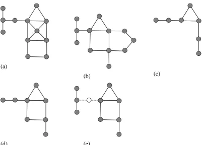
Figure 1: (a) and (b) represent the graphs G1 and G2. (c), (d) and (e) are respectively the
MCIS, the cMCES and the dMCES for G1 and G2 (the white node in (e) is a feature from G1,
and has been included for ease of understanding but is not part of the dMCES).
The Maximum Common Induced Subgraph (MCIS), as shown in Figure 1c above, is
the largest (in terms of the number of vertices) induced subgraph common to G1 and G2,
whereas the Maximum Common Edge Subgraph (MCES) is the largest (in terms of the
number of edges) induced subgraph common to G1 and G2. There are two types of MCES:
the connected MCES (cMCES) and the disconnected MCES (dMCES), as shown in Figures
1d and 1e respectively. A cMCES is one in which each constituent vertex is connected by at
least one path in the graph, i.e., the MCES consists of a single, connected subgraph; in a
dMCES, conversely, this condition does not hold and the MCES can hence contain two or
more subgraphs.
3.
Cliques, modular products and colouring
A clique is a set of vertices in a graph such that each vertex is connected to each and every
[image:4.595.71.475.86.374.2]4
larger clique and with the maximum clique being the maximal clique with the greatest number
of vertices. Levi [12] and Barrow and Burstall [13] appear to have been the first to realise
that algorithms for the detection of maximum cliques could be used to identify the MCIS
(and thus the MCES) by using the modular product of the two line graphs describing G1 and
G2. As will be seen in Section 4, the modular product forms the basis for several important
MCS algorithms that are based on clique detection.
The modular product of two graphs, sometimes referred to as a compatibility graph, is
a graph with the vertex set V1 × V2 of graphs G1 and G2 respectively. If the edge set of G1 is
E(G1), where an edge is a pair of vertices (e.g. (ui,uj)), and analogously for G2, E(G2) and
(vi,vj), then an edge between two vertices exists in the modular product where
(ui,uj) E(G1) and (vi,vj) E(G2) or,
(ui,uj) E(G1) and (vi,vj) E(G2).
The maximum clique(s) in the modular product then correspond to the MCIS between the
two graphs [14]. In weighted and labelled graphs, an additional condition applies such that
only vertices of the same label are matched, and likewise for the edges, i.e:
w(ui,uj) = w(vi,vj),
where w() denotes the vertex and edge labels for a pair of vertices comprising an edge.
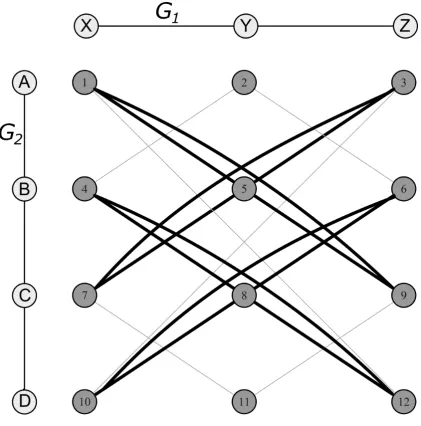
The module product is described in Figure 2, where it will be observed that edges
exist between vertices of the modular product when an edge exists for G1 for a given pair of
vertices, and an edge also exists for G2. Vertices A and B in G2 and X and Y in G1 show this,
since an edge exists between both A and B in G2, and X and Y in G1, thus giving rise to an
edge between vertices 1 and 5. An edge also exists between vertices 1 and 12, since no edge
exists between the corresponding G2 vertices A and D, and neither is there an edge between
X and Z in G1. No edge, however, exists between vertices 1 and 6, for whilst there exists an
edge between A and B in G2, vertex X is not joined to vertex Z in G1. Four cliques (and two
unique MCISs) are highlighted in the figure, e.g., the clique (4,8,12) corresponds to the MCIS
involving vertices (B,C,D) in G1, and (X,Y,Z) in G2.
The procedures described above find the MCIS, as is the case with many published
MCS algorithms. However, the MCES better describes the notion of chemical similarity, and
finding the MCES is computationally simpler than finding the MCIS. This is because in the
former case, one must take into account both vertex and edge labels, rather than just vertex
labels as in the MCIS, with the result that the modular product will contain fewer vertices and
5
MCES using a theorem due to Whitney [15] (as discussed by by Raymond et al. [9] and by
6
Figure 2: Modular product of two graphs G1 and G2, where G1 is a linear connection of three
vertices (X, Y and Z) and G2 a linear connection of four vertices (A, B, C and D). Edges in
bold are part of the four cliques that exist, whereas edges in light grey are not part of these
cliques. The numbers have been assigned to each node of the modular product for referencing
purposes.
et al. [16]), who showed that it is possible to reconstruct a graph from its respective line
graph, and vice versa. By analogy, it is thus possible to construct the MCES from the MCIS
by constructing a modular product from the line graphs instead of the original graphs. In this
case, a vertex in the modular product will now represent an edge match between the two
original graphs, instead of a vertex match. It should be noted that there is one exception to
7
isomorphic edge-graphs and hence to erroneous results for the MCES when translating back
from line graphs to the original graphs: however, such results are easy to identify and prune,
hence ensuring the identification of the correct MCES [17-19].
It will be clear from the above that the modular product graph constructed from two
molecular graphs can be large, and more importantly, have a high edge density. The latter is
a direct result of the sparseness in degree of chemical graphs, and leads to a more
time-consuming search process for clique detection algorithms. The time requirements can be
substantially reduced by simplifying the modular product, but this needs to be done without
removing chemical meaning and without reducing the size of the MCS that is identified. To
this end, Kawabata [20] introduced what he referred to as the topologically-constrained
dMCS (tdMCS) (a concept that has parallels in several older publications [21-23]). Although
the conventional dMCS is suitable for mapping multiple disconnected fragments between two
molecules, no constraints on the distance between the fragments are considered, which can
yield alignments that are unlikely (or even nonsensical) in some cases. The tdMCS has the
attractive property of producing a dMCS that can involve more realistic alignments, and is
faster to calculate than a conventional dMCS.
The tdMCS is based on the topological distance T(a,b) between two atoms (or edges)
a and b, i.e., the minimum path distance between two features in a graph. The tdMCS is the
dMCS resulting from the application of the following constraint when constructing edges in
the modular product graph for two graphs A and B:
TA(ai, bi) – TB(aj, bj)≤ for 1 ≤ i < j ≤ m.
Here, represents a threshold on the maximum allowed difference in distance between two
pairs of vertices (or edges), and |m| represents the number of vertices in the modular product
graph. Any edge in the modular product that violates this constraint is deleted, and the
resulting maximal clique(s) correspond to tdMCSs. Kawabata found that the tdMCIS yielded
better agreements with alignments of superimposed ligands in ligand-protein structures than
did the dMCIS [20]. Related work has been reported by Klinger and Austin [22] and by
Raymond et al. [24]. Klinger and Austin described a neural network algorithm to identify
two types of MCS that were referred to as “bond types” (which was similar to a dMCIS) and
“topological
8
significantly reducing the required search time by deleting both vertices and edges from the
[image:9.595.77.536.134.328.2]modular product graph.
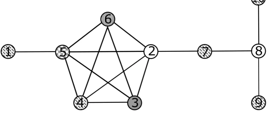
Figure 3: Example of a coloured graph that contains a clique, with vertices {2, 3, 4, 5, 6}).
The chromatic number here is 5.
A further important component of many clique-based MCS algorithms is the concept of
graph colouring, an NP-complete problem that originally arose from the need to colour the
countries on a map so that no neighbouring countries would be the same colour.
Mathematically, graph colouring (of vertices) can be represented as a function c(v) for a
given vertex v, such that c(v1) c(v2) when (v1,v2) E(G). As with maps, each vertex must
have a colour that is different from its neighbours’ colours, and the smallest number of
unique colours in a graph is denoted by its chromatic number (which is sometimes written as
(G) for a graph G) [11]. The use of graph colouring for clique detection is exemplified in
Figure 3, where all the vertices in a clique have different colours. Thus, a clique can be
easily detected by showing that all of the neighbours of a given node possess different
colours, a fact that forms the basis for several clique detection algorithms.
4.
Algorithms based on clique detection
Having introduced the relationship between maximum cliques and MCSs, we now describe a
range of algorithms that are based on cliques, with others being discussed in earlier reviews
9
In its simplest form, a backtracking clique detection algorithm involves traversing a
search tree based on the following recursive definition [9]:
(G) = max{1 + (NG(v)), (G\v)}.
Here, (G) is the maximum clique of graph G (which is usually the modular product in this
context), NG(v) is the set of vertices adjacent to vertex v in G, and G\v is graph G with vertex
v deleted. A pseudocode version of this basic algorithm is shown in Figure 4 (an efficient,
non-recursive version of this algorithm is described by Carraghan and Pardalos [27]). Here,
the vertices in G are processed in ascending order of degree, where v1 has the smallest degree
in G, v2 has the smallest degree in G\v1, and vk is the vertex of smallest degree in G\{v1,...,v
k-1}.
4.1 Bron-Kerbosch
The Bron-Kerbosch algorithm [28], which is shown in its simplest, recursive form in Figure
5, has been widely used in chemical and life science applications since an early comparison
of several algorithms by Brint and Willett [29]; indeed, over one-third of the 735 citations in
the Web of Science Core Collection database to Bron and Kerbosch’s 1973 article come from
chemical or life science journals (with the Journal of Chemical Information and Modeling
being the second-largest single source of citations). It will be realised that their algorithm is
very similar to the basic procedure shown in Figure 4 in that it recurses through
neighbourhoods of selected vertices in the graph. There are, however, two major differences
that have caused it to be widely used. First, it keeps track of previously-used vertices
(represented as X in the figure), hence substantially increasing performance by the avoidance
of futile backtracking; second, it reports all of the maximal cliques that are found, and not just
a single maximum clique. A modification of the algorithm by the same authors, and more
formally defined by Cazals and Karande [30], involves the selection of a pivot vertex from P
X and consideration for clique exploration only those vertices that are not adjacent to this
pivot vertex.
Koch [17] developed three extensions to the Bron-Kerbosch algorithm, all of which
relied on removing redundant cliques that did not contribute to finding the MCS when using
the modular (or edge) product of two graphs. These extensions were based on the concept of
a c-edge, something that is described most readily if we consider the modular product of a
10
and (e2,f2) possess a common vertex, where (e1,e2) is an edge in G1 and (f1,f2) is an edge in G2.
In this case for clique detection, G1 is isomorphic to G2. A clique is spanned by a connected
11 Data: vertex set G (of modular product), current clique C, max clique (G)
Result: Maximum Clique (G)
Function FindCliques(G):
While G is not empty do
select v from G;
C = C v;
FindCliques(NG(v)) ;
If |C| > | (G)| then
(G) = C
end
G = G\v ;
end
Figure 4: A simple backtracking maximum clique-detection algorithm
Data: vertices in clique R, current vertex set (of modular product graph) P,
previously-processed vertices X
Result: Maximal Cliques C
Function BK(R,P,X):
If P is empty and X is empty then
add R to C ; // A maximal clique has been found
end
else
for vertex v P do
BK(R v, P NG(v), X NG(v)) ;
P = P v ;
X = X v ;
end
end
12
connected c-edges, and then translated the set to the relevant vertices in the parent graph to
yield the maximum clique in G. The maximum clique of the c-edges, a c-clique, corresponds
to the cMCES between the two graphs, and Koch found that this simple modification was
significantly faster than the standard Bron-Kerbosch algorithm. This algorithm, despite the
above description, can be applied to non-isomorphic graphs and thus yields the maximal
c-cliques between the two graphs.
A further development of this basic approach is described by van Berlo et al. [31],
who extended the Bron-Kerbosch algorithm and Koch’s c-edge approach to find the maximal
clique corresponding to the cMCIS and cMCES. This is achieved using several heuristics
that were applied to improve search times. For example, the algorithm orders vertices in the
search tree based on their “centrality” (an average of the shortest path lengths to every other
node in the modular product), where those that are most central are selected first. Another
heuristic is the application of 68 atom-types that are used to label the atoms in the two
molecules that are being compared. An initial MCS is found by matching based on these
atom types and the resulting mapping is then used to seed the search for the actual MCS, in
which the atomic symbol is used as the label.
4.2 TOPSIM
TOPSIM [18] is an MCES-finding algorithm that relies on finding the maximum clique in a
reduced compatibility graph of the line graphs of two weighted graphs, where a reduced
compatibility graph is constructed where vertices are made only for matching atom and bond
labels. A node in the modular product here is labelled as (e, e ) where e is an edge from G1
and e is an edge from G2 with the same edge label, and the vertices on the edge both have the
same labels as in e. Edges between these vertices are constructed in the same way as with the
modular product, and, like the modular product, the maximum clique corresponds to the
MCES. A branch-and-bound algorithm was employed for clique detection in TOPSIM.
Starting from the root, the depth-first algorithm explores each node of the tree (which
represents a vertex in the reduced modular product). The next node chosen in the tree is
considered legal if it is connected to every other node in the clique identified so far (or if no
clique has been found, the first node is selected by default). Once all possible vertices in a
path have been explored, the algorithm backtracks, deleting vertices and exploring different
paths in the same branch (or perhaps exploring a different branch of the tree), with the largest
13
the algorithm is the maximum clique determined from a pruned version of the reduced
modular product (the pruning will not be discussed, though it aimed to preserve edges which
had identical neighbouring edges in both graphs) while the upper bound is the maximum
possible clique size.
4.3 Babel
Babel [32] described an early colouring algorithm for finding the maximum weighted clique
of a graph. The algorithm starts initially with a random vertex, and then starts assigning
colours such that neighbours do not possess the same colour. The next vertex chosen in the
graph is the one with the greatest number of colours already assigned to its neighbours, in
effect colouring vertices in a localised order of degree. The maximal cliques are found using
a branch-and-bound algorithm in which the upper and lower bounds are the largest assigned
colour for a vertex and the weight of the heaviest clique found over the course of the
algorithm, respectively. The basic concept underlying the algorithm is that if a vertex is in a
clique then the number of colours assigned to its neighbours must be equal to, or greater than
the number of colours in the greatest clique found thus far: if this is not the case then that
vertex is eliminated from the graph being studied.
4.4 RASCAL
Raymond et al. developed the algorithm RASCAL (for RApid Similarity CALculation) for
graph-based similarity searching in chemical databases, as well as for chemical MCES
detection [19, 24]. RASCAL relies on an initial screening process to significantly boost the
speed of searching, eliminating a large fraction of the molecules in a database so that the
computationally demanding graph search is only performed when a pair of molecules are
similar enough to suggest that an MCS calculation is warranted. The screening stage
prefaces a branch-and-bound algorithm for finding cliques in the modular product of two line
graphs, with the condition that upon finding the MCES via the clique, the degree sequences
of the vertices of the relevant subgraphs are compared to ensure that a -Y exchange has not
occurred. The graph colouring used in RASCAL is referred to as node partitioning. Here,
vertices in the modular product are initially grouped into colours or “partitions” based on
whether they can actually be neighbours with each other. Given all the vertex pairs (vi, vj) in
14
G1 with n vertices would initially have n partitions. During each iteration of the clique
search, vertices remaining in the search tree can be re-assigned into other partitions based on
whether they are not neighbours to the existing vertices in a partition. This acts as a fast
method of shrinking the chromatic number, which also serves as an upper bound, as against
re-colouring the graph after each iteration. RASCAL utilises three different methods for
calculating the upper bound, based on the size of the candidate set of vertices to add to the
clique, and the calculated upper bound is the minimum of these three values at each stage
during the search. RASCAL also employs two pruning heuristics that attempt to remove
neighbouring vertices to a clique that could not possibly extend the clique, and to remove
symmetric vertices.
Barker et al. [21] used RASCAL to find the MCS in reduced graphs as a similarity
measure. Notably, the MCIS and MCES were used, and two types of reduced graph were
made. The first type were “topologically-connected” graphs, where only vertices connected immediately to each other were joined by edges in the reduced graph (in other words, a
standard reduced graph). The other was “fully connected,” where all vertices in the reduced graph were connected, and each edge was assigned a weight based on the shortest path length
from one node to the other in the topologically-connected graph (essentially, a tdMCS with
=0). A similar reduced-graph study by Takahashi et al. [23] allowed for overlapping
features in the reduced graph, and edges in the fully-connected reduced graphs could have
multiple weights (representing multiple paths from one feature to another, instead of simply
the shortest path).
4.5 Iterated local search
The iterated local search procedure of Grosso et al. [33] used neighbourhood rules to obtain a
maximal clique, with three fundamental aspects: movement operators; node penalisation; and
restart rules. The first operator is an "add" move, which augments the current clique with an
immediate neighbouring node not present in the clique. The other operator is a "swap" move,
which adds a node not adjacent to exactly one other node in the clique, and then removing its
neighbours in the clique, yielding an equal-sized clique to the previous one but transformed
to a different location in the given graph. Vertex penalties are assigned to a vertex whenever
it has already been featured in a clique computed from a previous iteration, where the penalty
is equivalent to the number of cliques it had featured in. Finally, the restart rules return a
15
in the entire graph, and its immediate neighbours, while a more complex rule involves only
performing such a restart if the move is guaranteed to remove a minimum fixed number of
vertices. It must be emphasised that this algorithm is non-deterministic, with most stages
relying on random selection to some degree: that said, and despite the fact that it is a maximal
(rather than maximum) clique algorithm, it was generally found to identify a maximum clique
in practice.
A modification of this algorithm has been used by Englert and Kovács [34] at
ChemAxon to give what is claimed to be the fastest inexact method for finding the dMCES
between two molecules. Their procedure seeks the maximum clique in the modular product
of two graphs using the algorithm of Grosso et al. [33], with several heuristics to improve the
time performance and to optimise the MCS that is returned upon completion of the clique
search. Two of these heuristics are applied to bias the search space. The first involves the
calculation of a “connectivity score” which represents the number of c-edges in a candidate node during clique expansion. Vertices with a higher connectivity score are selected, thus
biasing the search towards the detection of less fragmented MCSs. The second is a similarity
measure that is based on the Morgan algorithm and that calculates the maximum radius (in
topological distance) at which two vertices have identical circular environments. During
clique expansion, vertices are selected in the modular product with the highest weighted sum
of the scores from these two heuristics. In addition, the “labelled projection” upper bound for
the largest possible size of the dMCES described previously by Raymond et al. [19] is used
as an early termination criterion, with additional heuristics being employed to modify the
MCS post-clique search so as to improve the quality of the final mapping.
4.6 MaxCliqueSeq
The MaxCliqueSeq algorithm of Depolli et al. [35] is exact but involves an approximate
colouring method, albeit one that was found to be more robust in practice than that described
by Babel [32]. Starting from an initial colour, this colour is assigned to the highest-degree
vertex, instead of a randomly chosen one as is the case with the Babel algorithm. The
neighbours of this coloured vertex are then removed from a set dictating the vertices to
colour. Once this set becomes empty, it is refilled with uncoloured vertices, and the colour is
incremented to the next colour. The next vertex chosen for colouring is the first available in
the set, and the process is then repeated until all vertices are coloured. In addition to the use
16
order of degree prior to searching for cliques. The actual algorithm is a depth-first
backtracking algorithm, which relies on successive removal of non-neighbours and
identically-coloured neighbours to the current clique set. A pruning condition is used to
control the search:
|U| + |C| ≤ |Cmax|
where |U| is the size of the working set of vertices to explore, |C| is the size of the current
clique, and |Cmax| the size of the largest clique found thus far. Whenever this condition is
breached, the algorithm stops exploring that particular branch of the search tree. The speed
of the algorithm can be enhanced significantly by distributing the branch-and-bound search
tree across multiple cores as parallel processes, the resulting speed-ups being particularly
large when the algorithm is applied to the comparison of protein structures containing very
many amino acid residues.
5.
Other types of algorithm
While clique detection lies at the heart of many MCS algorithms, other approaches have been
described and some of these are reviewed in this section.
5.1 Subgraph enumeration algorithms
A conceptually simple approach to the detection of the cMCS involves enumerating all
connected subgraphs common to the two graphs that are being compared and then returning
the largest such subgraph. Perhaps the earliest use of this approach was described by
Armitage and Lynch in a study of techniques for the automatic indexing of the substructural
changes occurring in chemical reactions [36]. The algorithm commences by enumerating all
connected two-atom substructures in the two molecules that are being compared. Those
substructures that do not match (in terms of their atom and bond types) are discarded, and the
remaining substructures are then extended by one atom, and the atom and bond type filters
applied again. This extension-and-comparison process is continued until no common
subgraphs exist, at which point the common subgraph(s) from the previous iteration represent
the MCS(s). An important part of this algorithm (and of related ones adopting an analogous
approach) is the use of a fast canonicalisation procedure to ensure that identical subgraphs
17
Varkony et al. [37] extended the above algorithm by introducing multiple “similarity
definitions,” enabling users to produce MCSs which ignored atom and bond types, topology -type matching (i.e., ring atoms could not map to chain atoms) and even to take into account
the attachment points of a substructure in a molecule. An important feature of the algorithm,
and one that distinguishes it from those described thus far, was that it was specifically
designed to allow the comparison of not just two but multiple molecules, with the smallest
molecule under consideration being taken as the starting point for the enumeration. The
extension of this algorithm to 3D chemical graphs is described by Crandell and Smith [38].
The algorithm described by Takahashi et al. [39] is very similar to that of Varkony et
al. but used a faster method for identifying subgraph isomorphism, specifically the set
reduction technique first described by Sussenguth [40] and used for many years in chemical
substructure searching algorithms (though it has now been largely supplanted for that purpose
by the algorithm due to Ullmann that is briefly described in the next section). A recent
example of the enumeration approach is the fMCS algorithm of Dalke and Hastings [41].
Like its precessors, fMCS first deletes all atoms and bonds that are not in common between
the molecules being compared, yielding fragments. The largest fragment from each molecule
is taken, and the smallest of these largest fragments is tested for subgraph isomorphism in the
other molecule(s), and then extended. If this fails to yield the cMCS, the method then starts
with single bond fragments instead, which are enumerated from the input graphs.
Finally in this section we describe the MultiMCS algorithm of Hariharan et al. [42],
which is again designed so that it can handle more than two graphs at a time. This is based
on exhaustive enumeration, but differs from the other algorithms above in that it involves the
enumeration of all of the maximal common substructures for pairs of molecules, instead of all
of the substructures for a single molecule. One of the molecules is selected and this is then
matched in turn against each of the remaining molecules in turn, with the overall MCS then
being the intersection of all of resulting sets of maximal common substuctures. An analogous
strategy for handling multiple molecules based on the Bron-Kerbosch algorithm was
described by Brint and Willett [29] and subsequently by Martin et al. [43]; Hariharan et al.
instead developed a novel divide-and-conquer strategy that provides substantial speedups
when detecting all of the maximal common substructures for a given molecule-pair.
18
The MCS algorithm described by McGregor [44] employs a simple backtracking search but
reduces the number of backtrack instances necessary by inspecting the set of possible
solutions remaining at some point in the depth-first search and determining whether it is
necessary to extend the current solution. This is effected using a modification of the subgraph
isomorphism algorithm that was first described by Ullmann [45] and that now forms the basis
for most operational 2D and 3D chemical substructure searching systems [46]. The Ullmann
algorithm is based on a match matrix that initially encodes all possible equivalences between
the vertices comprising the two graphs that are to be compared, and this matrix is
progressively refined as definite vertex-to-vertex mismatches are identified during the
exploration of the search tree. When used for MCES detection in labelled and weighted
graphs, the match matrix encodes corresponding edges, rather than vertices. An ordering
scheme is used to modify the order of edges explored given the currently found common
subgraph, so as to maximise the number of corresponding edges between the two graphs as
soon as possible.
Although first described over three decades ago, the McGregor algorithm is of
continuing interest since it is an important component of the Small Molecule Subgraph
Detector (SMSD) Toolkit described by Rahman et al. [47]. This contains three different
MCS algorithms: one based on the implementation of the Bron-Kerbosch algorithm as
provided in the Chemical Development Kit [48]; one based on the algorithm of Cazals and
Karande [30]; and the third a subgraph isomorphism procedure that has been modified to
enable it identify approximate MCSs [47]. The choice of algorithm in a particular case is
based on the complexity of the two molecules that are to be compared, and the McGregor
algorithm is used in SMSD to check whether it is possible to further extend the MCSs
identified by the second and third of these three procedures.
5.3 consR
The approximate MCES algorithm described by Zhu et al. [49] uses an approach termed
anchor selection and expansion, which generates a match matrix between two large graphs.
The anchors here are vertices in the two graphs that possess a high similarity and
comparatively large degrees between the two graphs. Anchors are then expanded to match
neighbouring vertices that are highly similar, giving a list of possible candidate matches. The
most similar pair of vertices is registered in the match matrix, and any other candidate
19
assigned. These assigned vertices become anchors themselves for which neighbourhood
expansion is then repeated, until the whole graph has been analysed. A refinement of this
procedure uses minimal vertex covers; however, the identification of these is another
NP-complete problem so the authors used randomly-determined minimal vertex covers with the
result that their algorithm is non-deterministic in operation.
5.4 kCombu
The final algorithm to be described here is Kawabata’s kCombu algorithm, which circumvents the potentially costly requirement of constructing and searching the modular
product graph that is used in clique-detection MCS algorithms [20]. In the context of
generating the MCIS, pairs of vertices – one vertex in one graph and one vertex in the other –
are ranked based on a heuristic score. This score consists of three distances (so that the lower
the overall score, the better matched the two vertices are): a distance representing the
difference in the number of neighbours between two vertices; an extended-connectivity value
based on the Morgan algorithm; and a topological distance similar to the tdMCS constraint
described earlier.
A fixed number K of correspondences are generated (where the first element is one of
the top K pairs), and for each extension of each correspondence, the next best-scoring pair is
added, this process continuing until all (matchable) atoms have been used. The fact that
multiple correspondences are produced, means that up to K MCISs can be obtained (though
in practice several of these MCS results can be isomorphic).
6.
Conclusions
In this paper we have briefly summarised the principal characteristics of several algorithms
for MCS detection. It will be clear that MCS detection is a problem of continuing interest to
a range of academic disciplines, not least chemoinformatics, and we must emphasise that our
review has been necessarily selective given the vast literature associated with the subject.
In this concluding section, the reader might be expecting us to recommend some sort
20
several different types of MCS (even if one does not differentiate between MCIS and
MCES), with many of the algorithms being restricted to the detection of the cMCS. Second,
applications in chemoinformatics may require not only the maximum common subgraph but
also some or all of the maximal ones, this requirement precluding the use of those algorithms
that identify only the former. Third, algorithmic efficiency can be crucially dependent on the
size (in terms of the numbers of vertices and edges) of the graphs that are to be compared, on
their complexities (with highly symmetric graphs often proving problematic), and on the
degree of inter-graph similarity (where, e.g., back-tracking algorithms can be very slow if
there are many small common subgraphs present). Finally, and perhaps most importantly,
only a few papers report comparative experiments where two or more algorithms are applied
to the same set of molecules to ascertain their effectiveness, i.e., whether they do in fact find
the true MCS(s), and their efficiency, i.e., the time taken to achieve this. Even when such
comparisons are conducted, e.g. in the papers describing MultiMCS [42] and SMSD [47], it
is normal for only a few algorithms to be involved: it is hence to be hoped that more
extensive comparisons can be carried out in the future.
References
[1] D. Fooshee, A. Andronico, P. Baldi, ReactionMap: An efficient atom-mapping
algorithm for chemical reactions, J. Chem. Inf. Model. 53 (2013) 2812–2819.
[2] Y. Cao, T. Jiang, T. Girke, A maximum common substructure-based algorithm for
searching and predicting drug-like compounds, Bioinformatics 24 (2008) i366–i374.
[3] D. K. Agrafiotis, M. Shemanarev, P. J. Connolly, M. Farnum, V. S. Lobanov, SAR
maps: A new SAR visualization technique for medicinal chemists, J. Med. Chem. 50
(2007) 5926–5937.
[4] A. Sirageldin, A. Selamat, R. Ibrahim, Graph-based simulated annealing and support
vector machine in malware detection, in 5th Malaysian Conference in Software
Engineering (MySEC), 2011, pp 512–515.
[5] K. M. Borgwardt, C. S. Ong, S. Schonauer, S. V. N. Vishwanathan, A. J. Smola, H.-P.
Kriegel, Protein function prediction via graph kernels, Bioinformatics 21 (2005) i47–
i56.
[6] L. Han, R. C. Wilson, E. R. Hancock, A supergraph-based generative model, in 20th
21
[7] E. Duesbury, J. D. Holliday, P. Willett, Maximum common substructure-based data
fusion in similarity searching, J. Chem. Inf. Model. 55 (2015) 222–230.
[8] T. Kawabata, H. Nakamura, 3D flexible alignment using 2D maximum common
substructure: Dependence of prediction accuracy on target-reference chemical
similarity, J. Chem. Inf. Model. 54 (2014) 1850–1863.
[9] J. W. Raymond, P. Willett, Maximum common subgraph isomorphism algorithms for
the matching of chemical structures, J. Comput. Aided Mol. Des. 16 (2002) 521–533.
[10] H.-C. Ehrlich, M. Rarey, Maximum common subgraph isomorphism algorithms and
their applications in molecular science: A review, Wiley Interdiscip. Rev. Comput. Mol.
Sci. 1 (2011) 68–79.
[11] R. Diestel, Graph Theory, 3rd ed.; Springer-Verlag, New York, 2006.
[12] G. Levi, A note on the derivation of maximal common subgraphs of two directed or
undirected graphs, CALCOLO 9 (1973) 341–352.
[13] H. G. Barrow, R. M. Burstall, Subgraph isomorphism, matching relational structures
and maximal cliques, Inf. Proc. Lett. 4 (1976) 83–84.
[14] D. Kozen, A clique problem equivalent to graph isomorphism, SIGACT News 10 (1978)
50–52.
[15] H. Whitney, Congruent graphs and the connectivity of graphs, Am. J. Math. 54 (1932)
150–168.
[16] V. Nicholson, C.-C. Tsai, M. Johnson, M. Naim, A subgraph isomorphism theorem for
molecular graphs, Stud. Phys. Theoret. Chem. 51 (1987) 226-230.
[17] I. Koch, Enumerating all connected maximal common subgraphs in two graphs,
Theoret. Comput. Sci. 250 (2001) 1–30.
[18] P. J. Durand, R. Pasari, J. W. Baker, C. Tsai, An efficient algorithm for similarity
analysis of molecules, Internet J. Chem. 2 (1999) 1–16.
[19] J. W. Raymond, E. J. Gardiner, P. Willett, RASCAL: Calculation of graph similarity
using maximum common edge subgraphs, Comput. J. 45 (2002) 631–644.
[20] T. Kawabata, Build-up algorithm for atomic correspondence between chemical
structures, J. Chem. Inf. Model. 51 (2011) 1775–1787.
[21] E. J. Barker, D. Buttar, D. A. Cosgrove, E. J. Gardiner, P. Kitts, P. Willett, V. J. Gillet,
Scaffold hopping using clique detection applied to reduced graphs, J. Chem. Inf. Model.
46 (2006) 503–511.
[22] S. Klinger, J. Austin, Chemical similarity searching using a neural graph matcher, in
22
[23] Y. Takahashi, M. Sukekawa, S. Sasaki, Automatic identification of molecular similarity
using reduced-graph representation of chemical structure, J. Chem. Inf. Comput. Sci. 32
(1992) 639–643.
[24] J. W. Raymond, E. J. Gardiner, P. Willett, Heuristics for similarity searching of
chemical graphs using a maximum common edge subgraph algorithm. J. Chem. Inf.
Comput. Sci. 42 (2002) 305–316.
[25] E. J. Gardiner, P. J. Artymiuk, P. Willett, Clique-detection algorithms for matching
three-dimensional molecular structures. J. Mol. Graph. Model. 15 (1997) 245–253.
[26] P. M. Pardalos, S. Rebennack, Computational challenges with cliques, quasi-cliques and
clique partitions in graphs, Lect. Notes Comput. Sci. 6049 (2010) 13–22.
[27] R. Carraghan, P. M. Pardalos, An exact algorithm for the maximum clique problem,
Oper. Res. Lett. 9 (1990) 375–382.
[28] C. Bron, J. Kerbosch, Algorithm 457: Finding all cliques of an undirected graph,
Commun. ACM 16 (1973) 575–577.
[29] A. T. Brint, P. Willett, Algorithms for the identification of three-dimensional maximal
common substructures, J. Chem. Inf. Comput. Sci. 27 (1987) 152-158.
[30] F. Cazals, C. Karande, A note on the problem of reporting maximal cliques, Theor.
Comput. Sci. 407 (2008) 564–568.
[31] R. J. P. van Berlo, M. J. L. de Groot, M. J. T. Reinders, D. de Ridder, D. Efficient
Calculation of Compound Similarity Based on Maximum Common Subgraphs and Its
Application to Prediction of Gene Transcript Levels, at
http://bioinformatics.tudelft.nl/sites/default/files/ict2009-01.pdf
[32] L. Babel, A fast algorithm for the maximum weight clique problem, Computing 52
(1994) 31–38.
[33] A. Grosso, M. Locatelli, W. Pullan, Simple ingredients leading to very efficient
heuristics for the maximum clique problem, J. Heuristics 14 (2008) 587–612.
[34] P. Englert, P. Kovács, Efficient heuristics for maximum common substructure search, J.
Chem. Inf. Model. 55 (2015) 941–955.
[35] M. Depolli, J. Konc, K. Rozman, R. Trobec, D. Janežič, Exact parallel maximum clique
algorithm for general and protein graphs, J. Chem. Inf. Model. 53 (2013) 2217–2228.
[36] J. E. Armitage, M. F. Lynch, Automatic detection of structural similarities among
chemical compounds, J. Chem. Soc. C (1967) 521–528.
[37] T. H. Varkony, Y. Shiloach, D. H. Smith, Computer-assisted examination of chemical
23
[38] C. W. Crandell, D. H. Smith, D. H. Computer-assisted examination of compounds for
common three-dimensional substructures, J. Chem. Inf. Comput. Sci. 23 (1983)
186-197.
[39] Y. Takahashi, Y. Satoh, H. Suzuki, S. Sasaki, Recognition of largest common structural
fragment among a variety of chemical structures, Anal. Sci. 3 (1987) 23–28.
[40] E. H. Sussenguth, A graph-theoretic algorithm for matching chemical structures, J.
Chem. Doc. 5 (1965) 36-43.
[41] A. Dalke, J. Hastings, FMCS: a novel algorithm for the multiple MCS problem. J.
Cheminf. 5 (2103), at
http://jcheminf.springeropen.com/articles/10.1186/1758-2946-5-S1-O6
[42] R. Hariharan, A. Janakiraman, R. Nilakantan, B. Singh, S. Varghese, G. Landrum, A.
Schuffenhauer, MultiMCS: A fast algorithm for the maximum common substructure
problem on multiple molecules. J. Chem. Inf. Model. 51 (2011) 788–806.
[43] Y. C. Martin, M. G. Bures, E. A. Danaher, J. DeLazzer, I. Lico, P. A. Pavlik, A fast
new approach to pharmacophore mapping and its application to dopaminergic and
benzodiazepine agonists, J. Comput.-Aided Mol. Des. 7 (1993) 83-102.
[44] J. J. McGregor, Backtrack search algorithms and the maximal common subgraph
problem, Software Pract. Exper. 12 (1982) 23–34.
[45] J. R. Ullmann, An algorithm for subgraph isomorphism, J. ACM 16 (1976) 31-42.
[46] A. R. Leach, V. J. Gillet, An Introduction to Chemoinformatics, 2nd ed., Springer,
Dordrecht, 2010.
[47] S. A. Rahman, M. Bashton, G. I. Holliday, R. Schrader, J. M. Thornton, Small molecule
subgraph detector (SMSD) toolkit, J. Cheminf. 1 (2009) 12.
[48] C. Steinbeck, Y. Han, S. Kuhn, O. Horlacher, E. Luttmann, E. Willighagen, The
chemistry development kit (CDK): An open-source Java library for chemo- and
bioinformatics, J. Chem. Inf. Comput. Sci. 43 (2003) 493–500.
[49] Y. Zhu, L. Qin, J. X. Yu, Y. Ke, X. Lin, High efficiency and quality: large graphs