White Rose Research Online
[email protected]
Universities of Leeds, Sheffield and York
http://eprints.whiterose.ac.uk/
This is a copy of the final published version of a paper published via gold open access
in
International Journal on Software Tools for Technology Transfer
.
This open access article is distributed under the terms of the Creative Commons
Attribution Licence (
http://creativecommons.org/licenses/by/4.0/
) which permits
unrestricted use, distribution, and reproduction in any medium, provided the
original work is properly cited.
White Rose Research Online URL for this paper:
http://eprints.whiterose.ac.uk/85886
Published paper
DOI 10.1007/s10009-015-0378-x
R E G U L A R PA P E R
MCMAS: an open-source model checker for the verification
of multi-agent systems
Alessio Lomuscio1 · Hongyang Qu2 · Franco Raimondi3
© The Author(s) 2015. This article is published with open access at Springerlink.com
Abstract We present MCMAS, a model checker for the verification of multi-agent systems. MCMAS supports effi-cient symbolic techniques for the verification of multi-agent systems against specifications representing temporal, epis-temic and strategic properties. We present the underlying semantics of the specification language supported and the algorithms implemented in MCMAS, including its fair-ness and counterexample generation features. We provide a detailed description of the implementation. We illustrate its use by discussing a number of examples and evaluate its performance by comparing it against other model checkers for multi-agent systems on a common case study.
Keywords Verification·Multi-agent systems·Model checking
1 Introduction
Model checking [15] is widely recognised as one of the lead-ing logic-based techniques for the verification of reactive systems [54]. In this paradigm, a system S is encoded as a
B
Alessio LomuscioHongyang Qu [email protected]
Franco Raimondi [email protected]
1 Department of Computing, Imperial College London,
London, UK
2 Department of Automatic Control and Systems Engineering,
University of Sheffield, Sheffield, UK
3 School of Science and Technology, Middlesex University,
London, UK
transition system, or model, MS by means of a programme
in a dedicated modelling language such as reactive mod-ules [1] or NuSMV [13]. A specificationPof the system is represented as a logical formulaφP. Verifying whether the systemSsatisfies the specificationPis encoded as the prob-lem of checking whether the model MSsatisfies the logical
formulaφP, formally written as MS | φP. Several
speci-fications of reactive systems, includingliveness,safetyand several specification patterns [20] of interest, can be encoded in discrete temporal logic, either in its linear variant LTL, or in its branching version CTL. Well-known extensions to this approach include employing real-time and probabilistic specifications [40,43].
The fundamental challenge in model checking is the so-calledstate-space explosion, i.e. the fact that the state space of a system grows exponentially with the number of variables employed to describe it. Various techniques have been devel-oped over the years to tame this difficulty including Binary Decision Diagrams, abstraction, bounded model checking, induction, and assume–guarantee reasoning, thereby result-ing in systems with state spaces of 1025 and beyond to be verifiable.
Specifically, epistemic logic [24], or logic of knowledge, has provided a natural and intuitive but yet formally sound and computationally attractive, framework for reasoning about security protocols [30], agreement protocols [66], knowledge-bases, etc. By adopting epistemic modalities as primitives, one can naturally express both private and col-lective (common, or distributed) knowledge of the agents in the system. For example, a security requirement concern-ing privacy or secrecy in a system run can be translated into a specification stating that no agent eventually knows the fact in question [64]. Similarly, mutual authentication, is naturally expressed by stating that a principal knows that another principal knows that some key is shared [5]. Sim-ilarly, an epistemic account can provide a natural set of specifications for cache-coherence protocols [4]. These are only some examples; we refer to the specialised literature for more examples [31,64].
It is therefore compelling to extend traditional model checking approaches so that they can support specifica-tions that include agent-based features. However, these are often sophisticated modal logics that may involve tailored fixed-points computations. So, novel labelling algorithms evaluating agent-based modalities need to be defined and integrated with those for the temporal logics of interest. In addition, since agent-based logics traditionally come equipped with a semantics that is finer-grained than plain Kripke models for temporal logic, input languages for the system description also need to be tuned to the needs of MAS. These include having an intuitive description of the states, actions, local protocols and local evolutions. These consid-erations suggest that adapting an existing model checking toolkit to the needs of the verification of MAS specified by epistemic and other logics inspired by MAS is not a simple exercise and may, in fact, result in more effort than building a dedicated one.
In this paper, we describe MCMAS, a model check-ing toolkit for the verification of MAS specified through a range of agent-based logics.MCMASuses Ordered Binary Decision Diagrams (OBDDs, [7]) for the symbolic repre-sentation of state spaces and dedicated algorithms for the computation of a number of epistemic operators encoding private and group knowledge and Alternating-time Tempo-ral Logic (ATL) operators. MAS are described inMCMAS by means of Interpreted Systems Programming Language (ISPL) programs, whose semantics is close to interpreted sys-tems, a popular framework in temporal-epistemic logic [24].
MCMAS is equipped with an Eclipse-based plug-in for coding support and offers a number of features typical of advanced model checkers, including the graphical represen-tation of counterexamples and witnesses, as well as fairness support.MCMASis released as open source [68] and has been used in several research projects worldwide. We here presentMCMASversion 1.2.2, which extends a previous
ver-sion [47] by means of more efficient algorithms to compute the state space and the labelling of formulas. Also, among other new features, more sophisticated treatment of uniform strategies, counterexamples and fairness constraints is now supported.
The rest of the paper is organised as follows. In Sect.2, we provide the formal underpinnings of the technique the model checker implements by giving the syntax and semantics of the logics employed as well as the algorithms implemented in the checker. In Sect.3we describe ISPL, the input to the model checker. Section4 describes the implementation and gives a few examples. Section5focuses on specific applications and reports experimental results. Section6describes related work and concludes the paper.
2 Symbolic model checking multi-agent systems
In this section, we give the theoretical foundations of MCMAS. We succinctly describe the semantics of inter-preted systems in Sect.2.1. We give the syntax of ATLK in Sect.2.2and provide model checking algorithms in Sect.2.3. We conclude in Sect. 2.4 by presenting the OBDD-based encodings for the algorithms.
2.1 Interpreted systems
At the heart of MCMAS and its modelling language is the notion of interpreted system as a formalisation of multi-agent systems. Interpreted systems were popularised by Fagin et al. [24] as a semantics for reasoning about knowledge; they can be extended to incorporate game theoretic notions such as those provided by ATL modalities. Here we loosely follow the presentation given in [47], where global transitions are given as the composition of local transitions.
We assume A P to be a set of atomic propositions and a set of agentsAg= {Ag0,Ag1, . . . ,Agn}for the system. We
often refer toAg0as the environment of the system.
Definition 1 (Interpreted systems) Given a set of agentsAg, an interpreted system is a tuple I S=({Li,Acti,Pi, τi}i∈Ag,
I,h)where:
– Li is a finite set ofpossible local statesfor agenti.
– Actiis a finite set ofpossible actionsfor agenti.
– Pi :Li →2Acti\∅is alocal protocolfunction for agenti
returning possible actions at a given local state.
– τi : Li × Act0 × · · · × Actn → Li is a
determinis-ticlocal transition functionreturning the local state for agenti resulting from the execution of ajoint actionat a given local state; we assume that every action is proto-col compliant, i.e. ifli=τi(li,a0, . . . ,ai, . . . ,an), then
– I ⊆L0×L1× · · · ×Lnis the set ofinitial global states.
– h⊆L0× · · · ×Ln×A Pis a labelling relation encoding
which atomic propositions are true in which state.
We say thatG=L0× · · · ×Lnis the set ofpossible global
statesfor the system andAC T =Act0×· · ·×Actnthe set of
possible joint actions. For a global stateg =(l0, . . . ,ln)∈G
and anyi ∈ Ag, we consider the functionli :G →Lisuch
thatli(g)=li, returning the local state of agentiin the global
stateg.
Observe that interpreted systems describe finite-state sys-tems composed of agents possibly synchronising with each other and the environment via joint actions. Also note that the local protocols implement the agents’ decision making and state the conditions for the transitions in the system. We refer to [24] for more details.
Interpreted systems naturally induce Kripke models which can be used to interpret our specification language. These are defined as follows.
Definition 2 (Induced models) Given an interpreted system I S = ({Li,Acti,Pi, τi}i∈Ag,I,h), the induced model of
I S (or simply the model) is a tupleMIS = (Ag,AC T, S,T,{∼i}i∈Ag\{Ag0},h)where:
– Agis the set of agents ofI S;
– AC T ⊆Act0× · · · ×Actnis the set of joint actions for
the systemI S;
– S⊆L0× · · · ×Lnis the set ofglobal states reachable
from I via T;
– T ⊆S×AC T ×Sis a transition relation representing the temporal evolution of the system. We assume that T is decomposable and define the transition relation as
(s,a,s)∈ T iff for alli ∈ Agwe haveτi(li(s),a))=
li(s);
– {∼i}i∈Ag\{Ag0}⊆S×Sis the set of equivalence relations,
one for each agent but not the environment, encoding the epistemic accessibility relations. For anyi ∈ Ag\{Ag0},
we assume that(s,s)∈∼iiffli(s)=li(s).
We use the notations →a sas a shortcut for(s,a,s)∈ T. We use the termpathto denote any sequence of states
π = (s0,s1, . . . ,sn, . . .) such that, for alli ≥ 0, we have
(si,a,si+1)∈ T for some actiona ∈ AC T. Given a path
π, we denote withπ(k)the state at positionk. Given a set of agentsΓ ⊆ Agand a joint actiona =(a0,a1, . . . ,an), we
denote withSΓ the projection ofSon the local states of the agents inΓ and withaΓ the tuple consisting of the elements inarestricted to the agents inΓ. In this case, we say thatais acompletionforaΓ. For instance, ifa=(a0,a1,a2,a3,a4)
andΓ = {1,3},aΓ = (a1,a3)andaAg\Γ = (a0,a2,a4).
GivenΓ ⊆ AgandAC T, the set AC TΓ denotes the set of all tuplesaΓ as above.
We say that a joint actiona ∈ AC T isenabledin a state s ∈ Sif there exists a states ∈ S such that(s,a,s)∈ T. Similarly, given a group Γ, we say thataΓ is enabled in a state if there exists a completion ofaΓ to a joint action a ∈ AC T such thata is enabled in that state. Note that, by Definition1, each component of an enabled action is locally protocol compliant. Further note that since a local action is always possible at any local state, the models considered are serial, i.e. there are no deadlocks.
Astrategyfor agentiis a functionσi :Li →2AC Ti\{∅}
such that ifai ∈ σi(li), thenai ∈ Pi(li). Given a group of
agentsΓ, astrategyforΓ is a functionσΓ :SΓ →2AC TΓ\ {∅} such that σΓ(lx1, . . . ,lxk) = (σx1(lx1), . . . , σxk(lxk)), whereσx1, . . . , σxkare strategies for the agentsx1, . . . ,xk ∈ Γ.
The strategies defined above are analogous to the non-uniform, incomplete information, memoryless strategies in [2]. Note that an agent (or a group of agents) adhering to memoryless strategies with incomplete information may perform different actions in different global states whose local component is the same. This allows for an element of action “guessing” that is not considered useful when reason-ing in terms of strategic abilities. In these cases, it is more meaningful to consider, still under incomplete information and memoryless assumptions, deterministicuniform strate-gies[37] of the formσi : Si → AC TΓ\∅, which restrict
the definition of strategy above by assuming that the same action is performed in the global states in which agentihas the same local state.
The model induced by an interpreted system is said to benon-uniform, i.e. along its paths the agents may pick dif-ferent actions, compatibly with their protocols, in the same local state at different global states. To evaluate an inter-preted system under theuniformityassumption, we consider the various (uniform) models derived from the induced non-uniform model in which along any path the agents select the same action whenever they are in the same local state. As we will see later, MCMAS supports the verification of both uni-form and non-uniuni-form models derived from an interpreted system.
2.2 Syntax of ATLK and satisfaction
collection of agents, knows about the system and each other (e.g. see [24] for an introduction to the area) and what a group of agents can collectively enforce in the system (e.g. see [65]). We illustrate this through some scenarios in Sect.5.
Definition 3 (Syntax of ATLK) The syntax of the logic ATLK is defined by the following BNF expression:
φ::= p| ¬φ|φ∨φ| Γ1Xφ| Γ1[φUφ] | Γ1Gφ|
Kiφ| EΓ2φ| DΓ2φ|CΓ2φ,
where p is an atomic proposition in A P,i ∈ Ag\{Ag0},
Γ1 ⊆ Agdenotes a set of agents andΓ2 ⊆ Ag, Γ2 = ∅,
denotes a non-empty set of agents.
Since, differently from [2], here we work with incomplete information, the meaning of the modalities depends on the uniformity assumption made on the system. If we do not assume uniformity, the reading of the ATL modalities is as follows. The formulaΓXφexpresses that the agents inΓ can ensure thatφholds at the next state irrespective of the actions of the agents inAg\Γ. In other words, the agents in Ag\Γ cannot ensure thatφis false at the next state.
The formulaΓGφconveys that it ispossiblethat the actions of the agents inΓ result inφbeing true forever in the future, irrespective of the actions of the agents inAg\Γ. As above, this means that the agents outsideΓ cannot ensureφ is not uniformly realised. Similarly, the formulaΓ[φUψ] signifies that the agents inΓ may be able to realiseψat some point in the future and to ensure thatφholds till then.
While the combination of incomplete information, knowl-edge and ATL modalities give rises to the readings above, we are generally interested in evaluating what the agents have the power to enforce by means of ATL formulas [2]. In our setting, this is the reading of the ATL operators under the assumption of uniformity.
In this case, the formulaΓXφis read as “groupΓ has a strategy to enforceφin the next state (irrespective of the actions of the agents not inΓ)”;ΓGφrepresents “group
Γ has a strategy to enforceφ forever in the future”; and Γ[φUψ]means “groupΓ has a strategy to enforce that
ψ holds at some point in the future and can ensure thatφ holds until then”.
The remaining operators are used to characterise epistemic states of agents as in [24]. In particular,Kiφis read as “agenti
knowsφ”,EΓφas “everybody in groupΓknowsφ”,DΓφas “φis distributed knowledge inΓ”, andCΓφas “φis common knowledge inΓ. It is known that the standard branching-time temporal operators E X,E G, and EU can be expressed by considering the “grand coalition of all agents”, e.g.E Xφ≡ AgXφ.
The satisfaction of ATLK specifications on induced mod-els is defined recursively as follows (recall that given an
action tuple aΓ for the agents only in Γ, we write a for any of the completions ofaΓ):
Definition 4 (Satisfaction) Given a modelM=(Ag,AC T, S,T,{∼i}i∈{1...n},h), a states0∈ S, and an ATLK formula φ, satisfaction forφinMat states0, formally(M,s0)|φ, is recursively defined as follows.
– (M,s0)| piffp∈h(s0);
– (M,s0)| ¬φiff it is not the case that(M,s0)|φ; – (M,s0)|φ1∨φ2iff(M,s0)|φ1or(M,s0)|φ2;
– (M,s0)| ΓXφiff there exists a strategyσΓ and an actionaΓ ∈σΓ(sΓ0)such that for all statess1such that s0 →a s1, we have(M,s1)|φ;
– (M,s0)| ΓGφiff there exists a strategyσΓ and an actionaΓ1 ∈σΓ(s0Γ)such that all statess1withs0 a
1
→s1 are such that there is an actionaΓ2 ∈σΓ(sΓ1)such that all statess2withs1 →a2 s2are such that, etc., and we have
that(M,si)|φ, for alli ≥0.
– (M,s0)| Γ[φ1Uφ2]iff there exists a strategyσΓ
and an actiona1
Γ ∈ σΓ(sΓ0)such that all statess1with s0 a
1
→ s1are such that there is an actionaΓ2 ∈ σΓ(sΓ1) such that all statess2withs1 a
2
→s2are such that, etc., and we have(M,sj)|φ2, for some j ≥0, and(M,si)|
φ1for all 0≤i < j.
– (M,s0)|Kiφiff for alls1∈Swe have that ifs0∼i s1
then(M,s1)|φ.
– (M,s0) | EΓφ iff for all s1 ∈ S we have that if s0
i∈Γ
∼i
s1then(M,s1)|φ.
– (M,s0) | DΓφ iff for all s1 ∈ S we have that if s0
i∈Γ
∼i
s1then(M,s1)|φ.
– (M,s0) | CΓφ iff for all s1 ∈ S we have that if s0
i∈Γ
∼i
+
s1, then(M,s1)| φ, where+ denotes the transitive closure of the relation.
We say that an interpreted system I S = ({Li,Acti,Pi, τi}i∈Ag,I,h)satisfies an ATLK specificationφif and only
prob-lem when combined with CTL or ATL [52]. Perfect recall semantics with ATL leads to an undecidable model checking problem [2].
2.3 Symbolic model checking ATLK
We now define model checking algorithms for the logic ATLK; these extend the corresponding ones for CTL [15]. The approach here presented is symbolic in that it uses Ordered Binary Decision Diagrams (OBDDs) [7] as basic data structures to encode sets of states and transitions.
For a given specification model, Algorithm 1 reports the high-level structure of the recursive model checking algo-rithm S AT(φ), returning the set of states of the model in whichφis true.
Algorithm 1Model checking algorithm for ATLK Input:φ.
Output:{s∈S|(M,s)|φ}. 1:if(φis an atomic proposition)then 2: return h(φ);
3:else if(φis¬φ1)then
4: return (S\S AT(φ1));
5:else if(φisφ1∨φ2)then
6: return (S AT(φ1)∪S AT(φ2));
7:else if(φisKi(φ1))then
8: return S ATK(φ1,i);
9:else if(φisEΓ(φ1))then
10: return S ATE(φ1, Γ );
11:else if(φisDΓ(φ1))then
12: return S ATD(φ1, Γ );
13:else if(φisCΓ(φ1))then
14: return S ATC(φ1, Γ ); 15:else if(φisΓX(φ1))then
16: return S ATAT L X(φ1, Γ );
17:else if(φisΓG(φ1))then
18: return S ATAT L G(φ1, Γ );
19:else if(φisΓ[φ1Uφ2])then
20: return S ATAT LU(φ1, φ2, Γ );
21:end if
The procedures S ATK,S ATE, and S ATD for the
epis-temic operators are described in Algorithms 2, 3, and 4. These take as input the sub-formula to be checked and return the set of states satisfying the epistemic formula.
They compute the existential pre-image of the set S AT(¬φ1)with respect to the appropriate epistemic relation,
i.e. the set of statesnotsatisfying the epistemic formula. The complement of this set with respect to the set of reachable statesSis the set of states satisfying the formula in question. Algorithm 5 iteratively calculates the set of states that can access a state not satisfyingφvia a finite sequence of epistemic relations for the agents inΓ. The complement of this set with respect toSis equal to the set of states satisfying CΓφ[60].
The algorithms for the ATL operators depend on the aux-iliary procedureAT L P R E(Γ,X)(see Algorithm 6), which computes the set of statesY ⊆S from which there exists a joint actionaΓ for the agents inΓ such that all action com-pletionsaofaΓ enabled at a state inY generate a transition to a state in X. Algorithm 7 employs this procedure directly to computeS ATAT L X, while Algorithms 8 and 9 implement
the standard fix-point algorithms.
Given the above, to compute whether an interpreted system I S validates a formula φ (without the uniformity assumption) we compute the induced modelMI Sand check whether I ⊆ S AT(φ). To compute whether an interpreted systemI Svalidates a formulaφunder uniformity, we estab-lish whether I ⊆ S AT(φ)on someMI Sinduced from I S under uniformity. The labelling for models generated under the uniformity assumption is also carried out using Algo-rithm 1; in this case the generation of the induced models accounts for the constraints on the actions.
Algorithm 2S ATK(φ,i)forKiφ.
1: X=S AT(¬φ);
2:Y= {s∈S| ∃s∈Xsuch thats∼is}; 3:return ¬Y∩S
Algorithm 3S ATE(φ, Γ )for EΓφ.
1: X=S AT(¬φ);
2:Y= {s∈S| ∃s∈Xsuch that∃i∈Γ,s∼is} 3:return ¬Y∩S
Algorithm 4S ATD(φ, Γ )forDΓφ.
1: X=S AT(¬φ);
2:Y= {s∈S| ∃s∈Xsuch that∀i∈Γ,s∼is}; 3:return ¬Y∩S
Algorithm 5S ATC(φ, Γ )forCΓφ.
1: X=S;Y =S AT(¬φ); 2:whileX=Ydo 3: X=Y;
4: Y= {s∈S| ∃s∈Xand∃i∈Γ such thats∼is}; 5:end while
6:return ¬X∩S
2.4 Symbolic model checking and OBDDs
Algorithm 6AT L P R E(Γ,X).
1:Z = {(s,aΓ) | s ∈ Sanda ∈ AC Tand∃s ∈ Xsuch that(s,a,s)∈T};
2:W = {(s,aΓ) | s ∈ Sanda ∈ AC Tand∃s ∈ S \ Xsuch that(s,a,s)∈T};
3:Y = {s| ∃a∈AC Tsuch that(s,aΓ)∈Z\W}; 4:return Y
Algorithm 7S ATAT L X(φ, Γ )forΓXφ.
1:X=S AT(φ); 2:Y =AT L P R E(Γ,X); 3:return Y
Algorithm 8S ATAT L G(φ, Γ )forΓGφ. 1:X=S AT(φ);Z=S ATφ;Y =S;
2:whileX=Ydo 3: Y=X;
4: X=Z∩AT L P R E(Γ,X); 5:end while
6:return Y
Algorithm 9S ATAT LU(φ1, φ2, Γ )forΓ[φ1Uφ2].
1:X=S AT(φ2);Z=S AT(φ1);Y= ∅;
2:whileX=Ydo 3: Y=X;
4: X=Y∪(Z∩AT L P R E(Γ,X)); 5:end while
6:return Y
f1(x1,x2,x3)= ¬x1∨(x1∧ ¬x2∧ ¬x3), wherex1,x2,x3
are Boolean variables. The truth table of this formula is eight lines long. Alternatively, f1can be represented by means of
a binary tree with root nodex1, as in Fig.1, where the leaves
represent the truth value of f1. This tree can be simplified
as in Fig.2. Notice that the simplified tree only has 5 nodes instead of 15. In general, thereducedtree can be orders of magnitude smaller than the truth table for a given Boolean formula.
Symbolic model checking exploits the compression capa-bilities of OBDDs to represent large state spaces efficiently. A Boolean formula can represent a state in a model. As an example, consider a model in whichS = {s0,s1, . . . ,s7}.
The Boolean formula f0(x1,x2,x3) = x1 ∧x2 ∧ x3 can
be used to encodes0, the Boolean formula f1(x1,x2,x3)=
¬x1∧x2∧ x3to encode s1, etc. The number of Boolean
variables required to encode a setSgrows asO(log2(|S|)).
The set of states{s0,s1}can be represented by the
dis-junction of f0with f1. Boolean formulae can be encoded by
means of OBDDs; Algorithm 1 and all its associated proce-dures can operate on OBDDs, including the strategic (ATL) and epistemic modalities. We refer to [60] for more details about the encoding process.
x1
x2
x3
0 0
0 1
x3
0 1
0 1
0 1
x2
x3
1 1
0 1
x3
1 1
0 1
0 1
0 1
Fig. 1 The evaluation tree forf1(x1,x2,x3)= ¬x1∨(x1∧¬x2∧¬x3)
x1
x2
x3
0 1
1
0 1
1 1 0
Fig. 2 The OBDD for f1(x1,x2,x3)= ¬x1∨(x1∧ ¬x2∧ ¬x3)
3 Modelling multi-agent systems in ISPL
In this section, we describe Interpreted Systems Program-ming Language (ISPL), the language used to model MAS within MCMAS. ISPL is strongly based on Interpreted Sys-tems as defined in Sect.2. In this section, we present ISPL’s constructs and give its semantics.
An ISPL program describes a multi-agent system as com-posed of a number of agents and an environment. Agents’ definitions in ISPL closely follow those of agents in Def-inition 1. To describe an agent in ISPL we declare the following components. Local states are private, internal states of the agents, declared by means of variables, and cannot be observed by the other agents. Agents interact with each other and the environment by means of publicly observ-ablelocal actions. Actions are performed in accordance with a local protocol representing the agent’s decision-making process. Local states change value over time following a local evolution function, which returns the next local state on the basis of the current local state and the joint actions performed by all the other agents at a given instant. ISPL’s structure with actions and protocols is deliberately based on interpreted sys-tems’ semantics which constitute a widely used framework for describing MAS.
[image:7.595.47.293.49.401.2] [image:7.595.311.542.55.186.2]1 Agent Sender 2 Vars:
3 bit : {b0, b1}; -- The bit can be either 0 or 1 4 ack : boolean; -- True when the ack received 5 end Vars
6 Actions = {sb0, sb1, epsilon}; 7 Protocol:
8 bit=b0 and ack=false : {sb0}; 9 bit=b1 and ack=false : {sb1}; 10 ack=true : {epsilon}; 11 end Protocol
12 Evolution:
13 ack=true if (ack=false) and
14 ( ( (Receiver.Action=sendack) and 15 (Environment.Action=sendSR) )
16 or
17 ( (Receiver.Action=sendack) and 18 (Environment.Action=sendR) )
19 );
20 end Evolution 21 end Agent
Fig. 3 A simple ISPL example: the Sender Agent
randomly drop messages in either direction, but it does not modify the content of messages. To guarantee communica-tion, the Sender keeps sending the same bit to the Receiver until it receives an acknowledgement; at this point the Sender stops sending the bit. The Receiver performs no action until a bit is received, and keeps sending acknowledgements there-after.
Figure 3 reports the modelling of the agent Sender in ISPL. The declaration starts with the keywordAgent fol-lowed by a string identifier (the name of the agent). The variables declared in the Vars section (lines 2–5) define the local states of the agent. In this example, the Sender has four possible local states, corresponding to the possible combina-tions of the two variablesbitandack. ISPL also supports the declaration of bounded integers of the formx : a..b; whereaandbare two integer numbers (e.g.x: 1..4;). Actions are declared as an enumeration of identifiers (line 6). TheProtocolsection (lines 7–11) associates actions to sets of local states; for instance, line 10 represents the fact that when the variable ackis true, the agent must perform the actionepsilon. Sets of local states are charac-terised by Boolean conditions on local states. As an example, consider the Boolean condition ack=true on the vari-ableack: this corresponds to two local states, one where bit=b0and another wherebit=b1. Boolean expressions can also involve arithmetic expressions for integer variables (e.g.x>2 and x<5) and bit expressions for Boolean variables.
Non-deterministicprotocols are encoded in ISPL either by specifying more than one target action (see lines 7–10 in Fig. 5), or by giving different actions for overlapping conditions on local states. Observe that, differently from knowledge-based programmes [25], actions in ISPL are spec-ified on conditions on local states and not on the explicit knowledge that agents have. The ISPL sectionEvolution
1 Agent Receiver
2 Vars:
3 state : {empty, r0, r1};
4 end Vars
5 Actions = {epsilon,sendack};
6 Protocol:
7 state=empty : {epsilon};
8 (state=r0 or state=r1): {sendack};
9 end Protocol
10 Evolution:
11 state=r0 if ( ( (Sender.Action=sb0) and (state=empty)
12 and (Environment.Action=sendSR) ) or
13 ( (Sender.Action=sb0) and (state=empty)
14 and (Environment.Action=sendS) ) );
15 state=r1 if ( ( (Sender.Action=sb1) and (state=empty)
16 and (Environment.Action=sendSR) ) or
17 ( (Sender.Action=sb1) and (state=empty)
18 and (Environment.Action=sendS) ) );
19 end Evolution
20 end Agent
Fig. 4 A simple ISPL example: the Receiver Agent
1 Agent Environment
2 Vars:
3 state : {S,R,SR,none};
4 end Vars
5 Actions = {sendS,sendSR,sendR,sendNone};
6 Protocol:
7 state=S: {sendS,sendSR,sendR,sendNone};
8 state=R: {sendS,sendSR,sendR,sendNone};
9 state=SR: {sendS,sendSR,sendR,sendNone};
10 state=none: {sendS,sendSR,sendR,sendNone};
11 end Protocol
12 Evolution:
13 state=S if (Action=sendS);
14 state=R if (Action=sendR);
15 state=SR if (Action=sendSR);
16 state=none if (Action=sendNone);
17 end Evolution
18 end Agent
Fig. 5 A simple ISPL example: the Environment Agent
describes how the local states of an agent evolve over time (lines 12–20 of Fig. 3), using a syntax similar to the one employed in NuSMV [13]. For instance, lines 13–19 pre-scribe that thenextvalue of the variableackwill betrue if the current value of ack is false, agent Receiver is performing the actionsendack(see Fig.4), and the Envi-ronment agent is performing either the action sendSRor sendR(see Fig.5).
Figure4reports the full ISPL code for the Receiver agent. In this example, the unreliable channel is modelled by means of the Environment. Figure5reports the ISPL code for the Environment; notice (lines 7–10) that its protocol is non-deterministic.
[image:8.595.53.284.53.244.2] [image:8.595.308.541.58.219.2] [image:8.595.307.539.254.433.2]1 Agent Environment
2 Obsvars:
3 v3: boolean;
4 end Obsvars
5 Vars:
6 v1: boolean;
7 v2: boolean;
8 end Vars
9 [...]
10 end Agent
11
12 Agent A1
13 Lobsvars = {v1};
14 Vars:
15 [...]
16 end Agent
17
18 Agent A2
19 Lobsvars = {v2};
20 Vars:
21 [...]
22 end Agent
Fig. 6 A simple ISPL example: observable and partially observable variables
1 Evaluation
2 recbit if ( (Receiver.state=r0) or (Receiver.state=r1) );
3 recack if ( ( Sender.ack = true ) );
4 bit0 if ( (Sender.bit=b0) );
5 bit1 if ( (Sender.bit=b1) );
6 envworks if ( Environment.state=SR );
7 end Evaluation
Fig. 7 A simple ISPL example: atomic variables
agent only if they appear in theLobsvarsdefinition for that agent. For instance, agentA1in Fig.6can observe variable v1(but notv2), and agentA2can observe variablev2(but notv1). Both agents can observe variablev3. This feature enables faster communication and synchronisation between the agents and the environment.
Following the agents’ declarations, an ISPL model con-tains the sectionEvaluationdeclaring theatomic vari-ablesfor the model. Figure7 reports the definition of five atomic variables recbit, recack, bit0, bit1, envworks. The Boolean condition appearing on the right-hand side of each line denotes the set ofglobal states, where the propositions hold. The specifications to be verified (see theFormulaesection in Fig.8) are built on the propositions defined here.
The description of a system of agents is completed by providing a set of initial states, an optional set of fairness conditions, and the set of formulae to be verified. As shown in Fig.8, the set of initial states is declared in the section InitStatesby means of a Boolean function imposing conditions on local states. TheFairnesssection reports a list of Büchi fairness constraints, expressed as Boolean formulae. In the example of Fig.8, it is required that the propositionenvworks, which captures the fact the Envi-ronment is transmitting messages in both directions, must be true infinitely often: this means that the channel cannot block messages indefinitely. Finally, the sectionFormulae
con-1 InitStates
2 ( (Sender.bit=b0) or (Sender.bit=b1) ) and
3 ( Receiver.state=empty) and (Sender.ack=false) and
4 ( Environment.state=none);
5 end InitStates
6
7 Fairness
8 envworks;
9 end Fairness
10 11 Groups
12 g1 = {Sender,Receiver};
13 end Groups
14
15 Formulae
16 AG((recack and bit0) -> K(Sender,(K(Receiver,bit0))));
17 AG((recack and bit0) -> GCK(g1,bit0)));
18 end Formulae
Fig. 8 A simple ISPL example: initial states, groups, and fairness con-ditions
tains the specifications to be checked. These are formulas in the logic ATLK; since ATL subsumes CTL, formulas in the logics CTL or CTLK [59] are also supported. As an exam-ple, the first formula in Fig.8states that it is always true that, whenrecackis true and the value of the bit is 0, then the agent Sender knows that the agent Receiver knows that the value of the bit is 0. The second specification is stronger and states that whenrecackis true and the value of the bit is 0, it is common knowledge in the groupg1that the value of the bit is 0. The groupg1is defined above the specifications by the keywordg1, listing the groups of agents to be considered in the epistemic specifications for the model.
Semantics of ISPL programs Any ISPL program P uniquely denotes an interpreted systemI SP =({Li,Acti,Pi, τi}i∈Ag,I), obtained by instantiating the corresponding
ele-ments inI SP by means of the corresponding declarations in
P. More formally:
– The set of agents inI SP is the set of agents declared in
P, where the environment inPis mapped toAg0inI SP.
– For each agenti, the set of possible local statesLiinI SP
is defined by taking the Cartesian product of the corre-sponding sets defined for the local variables for agenti inP(SectionVars).
– For each agenti, the setActi is the corresponding set of
actions agentiin the programmeP(SectionActions). – For each agenti, the protocol Pi is defined by the list
of Boolean conditions in the SectionProtocolfor the agentiin the programmeP.
– For each agenti, the functionτi is defined by the list of Boolean conditions in the SectionEvolutionfor the agentiin the programmeP.
– The set of global initial statesIis defined by evaluating the Boolean conditions inInitStatesinP.
[image:9.595.50.142.58.231.2]evalu-ation h defined by the Boolean conditions in P (Section Evaluation). Formally, an ISPL program P satisfies a specificationφ(given in sectionFormulae) ifMI SP |φ. Note that since the semantics of ISPL programs is defined in terms of their corresponding interpreted system, their evo-lution is deterministic. Also observe that the composition of the different agents is synchronous via joint actions as in interpreted systems.
As described in Sect.2.1, under uniformity, an interpreted system induces not just one but a set of uniform models. In this case, we say that an ISPL programP satisfiesφunder uniform semantics if there exists an induced uniform model MI SP such thatMI SP |φ.
As an example, the model generated by the ISPL program for the bit transmission protocol is depicted in Fig.9, where:
– Global states are represented by rectangles; only the local states of the Sender and Receiver are reported, for readability the Environment is not. For instance, the global state((b0,false),empty)in the top-left cor-ner encodes a state in which variablebitfor the Sender has valuer0, variableackis false, and variablestate for the Receiver isempty.
– The temporal transitions are represented by solid arrows and for brevity are labelled with the Environment action only (the Sender’s and Receiver’s actions are derived deterministically from the protocol).
– The epistemic relations for the Sender are represented by dotted lines; dashed lines represent the epistemic rela-tions for the Receiver. All reflexive relarela-tions are omitted.
It can be manually checked that the first specification given is satisfied on the model; so the programme satisfies
it; whereas the second is false. This is in line with work in epistemic logic that establishes that common knowledge can-not be obtained in the presence of a faulty communication channel [24].
4 MCMAS: implementation and usage
MCMAS is implemented in C++ and can be compiled from its source code on most platforms (including Windows, Linux, Mac, Raspberry Pi and various other UNIX systems). The build recognises most architectures automatically. Pre-compiled versions of the tool are also available from the support pages [68]. In what follows, we describe MCMAS ver 1.2.2, released in March 2015.
4.1 Implementation details
To illustrate the tool, we discuss a number of implementa-tion choices that affect the overall performance ofMCMAS. In particular, we consider the following issues: (1) vari-able ordering in OBDDs; (2) computation of the set of reachable states; (3) construction of the temporal and epis-temic transition relations; (4) consistency checks of the input model.
4.1.1 Variable ordering in OBDDs
The size of an OBDD is very sensitive to the choice of the ordering for its Boolean variables. A good ordering can use less memory and speed up OBDD operations by orders of magnitude with respect to an alternative one. Finding a sta-tic ordering that generates a compact OBDD representation
((b0,false),empty) ((b0,false),r0) ((b0,true),r0)
((b1,false),empty) ((b1,false),r1) ((b1,true),r1) SendS
SendSR SendR
SendNone SendR
SendSR SendS
SendNone Send*
SendS
SendSR SendR
SendNone SendR
SendSR SendS
SendNone
Send*
Fig. 9 The model generated from the ISPL code for the bit transmis-sion protocol.Solid linesare temporal transitions labelled with actions (only the Environment action is reported); thedotted linesrepresent the
[image:10.595.77.521.512.655.2]for representing the state space and the transition relation is challenging. Dynamic reordering is a useful technique aimed at finding a good compromise between continuous variable reordering and efficiency with the aim of reducing memory consumption during model checking.
In some cases when the overhead of dynamic reorder-ing cannot be offset by its savreorder-ings, it may be more efficient to disable it completely, a feature supported by MCMAS. It is normally advantageous to provide heuris-tics for dynamic reordering tailored to specific models to reduce the overhead of evaluating all the possible orderings. The CUDD library [61] used by MCMAS allows group-ing OBDD variables so that the order of variables in the same group is not changed during reordering. This approach reduces the number of orderings that need to be explored. MCMAS provides four different initial OBDD grouping strategies:
1. Boolean variables for current and successor states are interleaved. The resulting ordering is: (v0, v0)· · ·(vn,
vn) X0, . . .Xn, wherev0, . . . vi0 are variables encoding
the local states for agent 0 and the other agents, and primed variables encode successor states. The variables X0. . .Xnencode actions and are grouped at the end.
2. A variation of the above whereby variables for actions are interleaved with states:(v0, v0)X0· · · (vn, vn)Xn.
3. For each agent, all the variables for the current state are grouped at the beginning, followed by the ables used to encode actions, followed by primed vari-ables to encode successor states: (v0, . . . , vi0)X0(v0,
. . . , v
i0) . . . (vinN+1, . . . , vn)Xn(viN+1, . . . , vn),
4. A variation of the case above whereby variables for the actions follow the variables for the states:(v0, . . . , vi0)
(v
0, . . . , vi0)X0· · ·(viN+1, . . . , vn) (viN+1, . . . , vn)Xn.
The first two strategies are similar to those used by NuSMV and other model checkers. The default OBDD order-ing strategy in MCMAS is the second one reported above, but, as we show later, some models benefit from the third and fourth heuristics.
4.1.2 Computing the set of reachable states
Let I S be an interpreted system andMIS = (Ag,AC T, S,T,{∼i}i∈{1...n},h)its induced model. In what follows the
functioni mage(x,T)returns the set of states accessible from xunder the transition relationT. MCMAS uses OBDDs to represent states and functions; the corresponding operations are conducted directly on OBDDs.
Algorithm 10Three approaches to compute reachable states 1: S⇐0;q⇐I;
2:whileS=qdo
3: S⇐q;q⇐S∪i mage(S,T); 4:end while
1: S⇐0;n⇐I;q⇐I 2:whileS=qdo
3: S⇐q;n=i mage(n,T);q⇐S∪n; 4:end while
1: S⇐0;n⇐I;q⇐I 2:whileS=qdo
3: S⇐q;n=i mage(n,T)\S;q⇐S∪n; 4:end while
MCMAS provides three approaches to compute the set of reachable states (see Algorithm 10). Experiments show that the time to construct OBDDs for reachable states by these approaches varies for different models and platforms (e.g. 32-bits Linux, 64-bits Linux, 32-bits Windows, etc.). No approach is consistently superior to the others. Note that MCMAS does not compute a single OBDD forT to avoid unnecessary computation time. Instead, the tool buildsn tran-sition relationsTi ⊆S×AC T×S,0≤i ≤n, one for each
agent and the environment; these are defined on the basis of the local transition functionsτ0, . . . , τn(see Definition1) as
follows:Ti(s,a,s)iffli(s)=τi(li(s),a). When the image
of xwith respect toT is needed, MCMAS executes a loop to construct the intersection ofT0, . . . ,Tnwithx, i.e.
y=x∩T0∩T1∩ · · · ∩Tn.
Note that x is also encoded over the whole set of OBBD variables, among which those for actions and successor states are abstracted away.
4.1.3 Building the temporal and epistemic relations It is often the case that the set of reachable states is only a small subset of the set of possible global states. While it may be time consuming to build a single OBDD for thecomplete transition relationTfor computing the reachable states, com-puting thepartial transition relation Tr each usually speeds
up the process when checking properties on reachable states. Formally,Tr eachis computed as follows:
Tr each =S∩T0∩T1∩ · · · ∩Tn,
whereSis the set of reachable states. In other words,Tr each
is the projection ofT on reachable states.
transition relationT, the computation of∼i is usually time
consuming. MCMAS employsvariable maskingto compute the OBDD encoding of the epistemic relations. For a setX of states, we compute the setY of indistinguishable state with respect to∼i as follows: letV be the set of all OBDD
variables encoding global states, andVi ⊆ V be the set of
OBDD variables encoding the local states for agenti. 1. We first compute an OBDD Xby removing the OBDD
variables inV\Vi, which are not part of agenti’s
encod-ing.Xis characterised by the following set:
X= {s∈L0× · · · ×Ln| ∃s∈X such thatsi=si},
wheresi andsiare the local states of agentiinsands,
respectively.
2. The OBDDYis computed asY =X∩S, whereSis the set of reachable states.
The above two steps can be performed efficiently using the procedures available in the CUDD library, and are applicable to Algorithms 3, 4 and 5.
For efficiency purposes, MCMAS implements optimised algorithms for the verification of CTL operators, rather than employing the procedures for the ATL modalities.
4.1.4 Fairness for ATLK
In a number of circumstances, it is desirable to remove cer-tain unwanted behaviours from the possible executions of a system. For instance, consider the code for the Environ-ment of the bit transmission protocol reported in Fig. 5. The protocol for this agent allows the environment to block messages forever; yet, the designer is likely to want to describe a situation in which the communication chan-nel randomly drops messages, but it is not continuously faulty.
The removal of unwanted behaviours is often achieved by imposingfairness conditions. In the case of branching log-ics such as ATLK, this requires the definition of constraints outside the model and the use of purpose-built verification algorithms which extend the standard labelling algorithm presented in Sect.2.3.
Fairness conditions are declared in MCMAS using an optional set of Boolean formulae constructed using atomic propositions from A P. In line with the standard literature, an infinite path in a model is said to befairif all the Boolean formulae from the set of fairness conditions are true infinitely often along the path.
MCMAS implements the standard algorithms for the ver-ification of temporal operators under fairness [15]. When the fairness options are enabled all operators are evaluated on the set of fair paths as discussed in [9].
4.1.5 Witnesses, counterexamples and strategy synthesis To assist with advanced validation support, MCMAS enables the user to inspect witnesses and counterexamples. These are provided astrees, instead of traces, adopting the algorithm described in [16]. MCMAS further extends [16] by:
1. by generatingfaircounterexamples and witnesses upon request. This is done by integrating the algorithm described in [14] for the temporal operators with the gen-eration of the counter-example tree;
2. by including additional cases for the additional operators. Algorithm 11 generates a counterexample for the formula Kiφ by picking a statenotsatisfyingφ (the remaining
epistemic operators are treated in a similar way). A sim-ilar algorithm can be used to compute a counterexample forKiφunder fairness by replacingS ATφis replaced by
S ATφFandSbySFin Algorithm 11. Algorithm 12 builds a witness for a formula of the formΓXφby comput-ing the setZof states in which agents not inΓ can move to a state satisfying¬φ, and returns an element from its complement. Algorithm 13, instead, returns a witness for a formula of the formΓφ1Uφ2. This algorithm
and a similar one for formulae of the formΓGφ(not reported here) follow the standard procedure for Until and Globally operators of CTL (see [15] for additional details).
Algorithm 11Counterexample forKiφin states.
1: X=S AT¬φ; 2:Y= {s∈S|s∼is}; 3:picksinY∩Xandreturns
Algorithm 12Witness forΓXφin states. 1: X=S AT¬φ;
2:Y= {(s,aΓ)| ∃s∈Ssuch that(s,a,s)∈T}; 3: Z= {(s,aΓ)| ∃s∈Xsuch that(s,a,s)∈T}; 4:pick(s,aΓ)inY\Zandreturn{s∈S|(s,a,s)∈T}
Algorithm 13Witness forΓφ1Uφ2in states.
1: P=S ATφ1;Q=S ATφ2;X= ¬(P∪Q); 2:W= {s}\Q;V= {s};
3:whileW= ∅do
4: Y= {(s,aΓ)|s∈W∧ ∃s∈Ssuch that(s,a,s)∈T}; 5: Z= {(s,aΓ)|s∈W∧ ∃s∈Xsuch that(s,a,s)∈T}; 6: Y=Y\Z;
7: pick(s,aΓ)inYandY1= {s∈S|(s,a,s)∈T};
8: W=Y1\(V∪Q);V =V∪Y1;
9:end while 10:return V
would require double-exponential algorithms and cause visu-alisation problems for the traces obtained.
Finally, it is customary for model checkers to compute counterexample for universal formulae that do not hold in a model, and witnesses for existential formulae that are true in a model. MCMAS extends this approach as follows (all formulae are assumed to be in negation normal form):
– MCMAS generates a counterexamples for universal for-mulas containing an existential formula. For instance, if the formulaAF E Gφis false, MCMAS generates a coun-terexample consisting a loop reachable from the initial state in whichE Gφdoes not hold.
– MCMAS generates a witness for existential formulas containing a universal formula. For instance, if the for-mula E F AGφ is true, MCMAS generates a witness consisting of a path leading from the initial state to a state in whichAGφholds.
– MCMAS generates witnesses or counterexamples for Boolean combinations of either universal or existential formulae (including the cases mentioned above).
MCMAS also provides limited support forstrategy syn-thesis for ATLK specifications. Strategy synthesis is the problem of deducing the strategies the agents need to employ so that a given specification is satisfied. Given an interpreted system and an ATLK specification over a set of agents inΓ, if the specification is satisfied, MCMAS can often return a witness model. This witness contains the actions that every agent inΓ performs at various states thereby making the for-mula true. The strategies of the agents inΓ can therefore be synthesised from the output. Note that the synthesised strate-gies are guaranteed to be protocol compliant due to how the model is generated.
4.1.6 Consistency checking
It is known that bounded integer types may generate over-flows in a reachable state. Due to the encoding strategy adopted inMCMAS, the value of a variable exceeding its upper bound is truncated to a value within its domain. This might lead to unexpected behaviours. To avoid thisMCMAS allows users to verify the presence of overflows as an optional check. This is carried out by encoding the transition relation Toverflowin such a way that an expression on the right-hand
side of an assignment is assumed to be beyond the bounds of the left-hand side variable, and then by constructing the con-junction ofToverflowand the reachable statesR. A non-empty
conjunction indicates the existence of an overflow.
The ISPL semantics requires that each state must have a successor state. So, checking deadlock states that do not have successor states is necessary to guarantee correct results of model checking, as deadlock states violate the premises of
the model checking algorithm forE G. Checking the presence of a deadlock state is implemented by model checking the formulaE G tr ueon the model. If the formula does not hold in all states, then there exists a deadlock state.
4.2 MCMAS usage
In its basic form the executable file mcmas is a standard command-line tool that takes as input the ISPL model to be verified. The executable accepts a number of command-line options, including:
– The options-o,-g, and-d are used, respectively, to select the algorithm to be used to order OBDD variables, to group OBDD variables, and to disable dynamic OBDD reordering.
– The option-eis used to select the algorithm to be used to generate the reachable state space (see Algorithm 10). – The options-kand-aare used to check for deadlocks
and arithmetic overflows in the model.
– The option-cis used to select the way in which coun-terexamples and witnesses are displayed. If this option is selected, the user can also tune the generation of coun-terexamples and witnesses using additional parameters provided using the options-p,-f,-l, and-w(we refer to the online documentation for a detailed description of these).
– The option-uniformis used to force the generation of uniform models as described in Sect.2.2.
MCMAS can also be used to performinteractive simula-tions: from the command line, this is achieved by invoking the tool with the-soption.
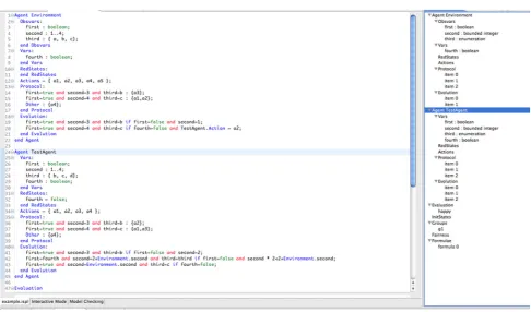
To improve usability, a graphical interface is available. The GUI is implemented as an Eclipse plug-in. The plug-in creates a new menu in Eclipse that guides the interaction. Currently, this interface supports the following features:
– ISPL program editingThis helps users create MCMAS projects and ISPL program skeletons; it implements syn-tax highlighting; it performs dynamic synsyn-tax checking (a separate ISPL compiler was implemented in Java + ANTLR [58] for this); it provides an outline view and the synchronisation between the outline view and the ISPL editor; it also supports text formatting and content assist.
Fig. 10 The ISPL Editor (Eclipse plug-in)
performed either explicitly, i.e. without OBDD encod-ing, or symbolically. The explicit simulation is performed by the Eclipse plug-in and does not require interaction with MCMAS. The symbolic simulation is more appro-priate for large models and requires the installation of MCMAS.
– VerificationIn this modality the GUI invokes MCMAS to execute the model checking procedures. Counterex-amples and witness traces are displayed in a graphic way using thedotutility from the Graphviz package [27]; states are shown as nodes and transitions as edges. When the mouse is rolled over a node in the graph, the cor-responding state is highlighted. The executions can be projected onto a subset of agents to mask unwanted infor-mation of other agents.
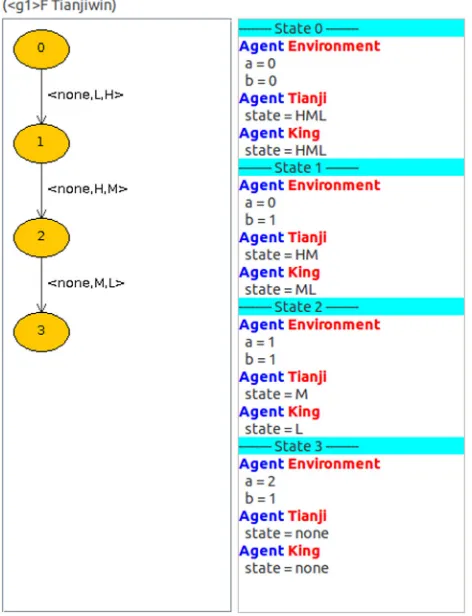
A screenshot of the Eclipse-based ISPL editor with syntax highlighting is shown Fig.10. A simple counterexample for a formula involving ATL operators is shown in Fig.11.
5 Scenarios and applications
In the past 10 years, MCMAS has been used to verify a wide number of systems ranging from simple multi-agent systems protocols to industrial scenarios [21–23,28,29,44,48–50]. In the following, we summarise a few instructive examples, but refer to the references above for more details.
The ISPL encodings for the scenarios below were either manually given, or automatically generated by means of dedicated compilers. While other traditional model check-ers could be used to model the scenarios, as we will see below, the specifications checked are based on epistemic or ATL formulas, hence normally not verifiable with traditional checkers.
We here focus on the tool functionality; the next section covers its performance when compared to other tools.
5.1 Example scenarios
We begin with simple scenarios from the artificial intelli-gence and MAS literature and then move on to describe more complex use cases.
5.1.1 The muddy children puzzle
Fig. 11 A model witness (Eclipse plug-in)
know and what they learn from each announcement it is pos-sible to show that at roundkthe muddy children say that they know they are muddy.
MCMAS can be used to verify that the children give the correct answer at each round, and have the correct knowl-edge at the end of the protocol. To do this we encode each child by means of an agent and use a set of initial states to generate a random assignment of muddy foreheads. We can then, for example, verify the specification stating that when a muddy child speaks, he indeed knows that he is muddy. This is captured by the formula below:
AG((muddyi∧saysknowsi)→ KChildimuddyi)
where the proposition “saysknowsi” is true after childisays
that he knows whether or not he is muddy.
Given the small size of the state space per child, the analy-sis can be performed on a very large number of children. Keeping track of the number of round of questions is not problematic but leads to a larger state space.
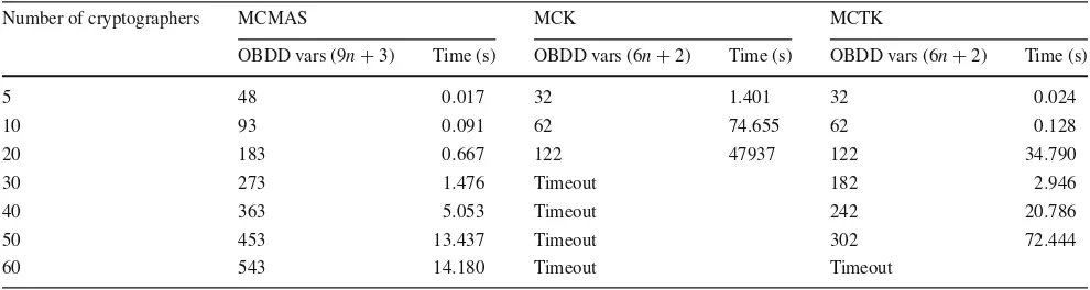
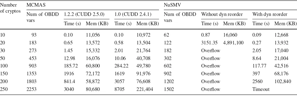
To evaluate the performance of MCMAS and the speed difference among various OBDD orderings, we ran MCMAS on a sequence of models increasing the number of children. All the experiments below and later were carried out on an AMD Phenom 9600B 2.3 GHz Processor with 8 GB
mem-ory running Linux kernel version 3.11.0-18. Any run that exceeded 24 h is reported as a timeout.
Table1shows that MCMAS is able to handle a large num-ber of children. The default OBDD ordering works well up to 100 children; ordering 3 and 4 are more efficient for the larger models.
5.1.2 One hundred prisoners
This puzzle concerns 100 prisoners kept in solitary confine-ment [19]. One day the warden gathers all the prisoners in the dining hall for dinner and announces that from the fol-lowing day he will randomly choose one prisoner every day for questioning. The interrogation room has only a light gov-erned by a toggle switch. Prisoners can observe whether the light is on when they enter the room. During their visit they are allowed to switch the light on or off as they please. While in the interrogation room, a prisoner may announce that he believes that all prisoners have already visited the interro-gation room. If a prisoner makes this announcement and this corresponds to the truth, then all prisoners are set free; if the announcement is not correct, all prisoners are exe-cuted. The prisoners are granted one meeting to coordinate their actions before the interrogations begin. It is assumed that prisoners can count days and that the light is initially off.
To check whether the puzzle’s solution is correct, we can model the prisoners’ behaviours, corresponding to the solu-tion of the puzzle, in ISPL and verify the formula
PrisonersF(Release) (1)
assuming Release to be true on the model only if all prison-ers are free. MCMAS finds the formula to be true thereby confirming the correctness of the solution. Table2 reports the performance of MCMAS on this example. As in the muddy children puzzle, we found that the default OBDD ordering is the most efficient when the model is small, while other orderings offer better performance on larger models.
5.1.3 Tian Ji racing horses
Table 1 Experimental results
for muddy children Number of children
Number of OBDD vars
Time (s)
OBDD ordrng 1
OBDD ordrng 2
OBDD ordrng 3
OBDD ordrng 4
20 111 0.61 0.50 0.76 0.76
40 213 11.46 6.57 8.76 10.68
60 313 40.29 39.58 54.16 97.67
80 415 165.62 144.44 190.46 192.49 100 515 736.04 431.85 466.05 385.31 120 615 920.02 1036.89 784.44 787.35
Table 2 Experimental results
for 100 prisoners Number of prisoners
Number of OBDD vars
Time (s)
OBDD ordrng 1
OBDD ordrng 2
OBDD ordrng 3
OBDD ordrng 4
5 40 0.40 0.34 0.41 0.43
10 88 13.79 13.00 11.50 11.48
15 123 118.23 122.57 126.75 126.93
20 161 1573.96 1692.87 1636.44 913.02
25 196 6541 8682 6083 7107
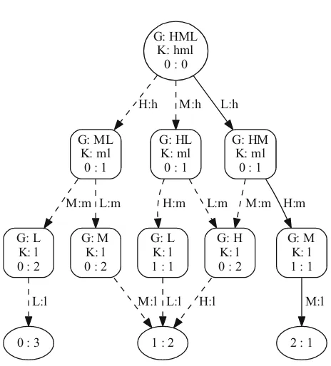
highest number of runs. However, for any given speed, the king’s horses always run faster than the general’s. Therefore, Tian Ji is always bound to loose the race, unless he cheats and employs horses in a different way. Tian Ji knows that the king will run the horses in the three races from the fastest to the slowest. MCMAS can be used to find the winning strategy for the general: we encode the king and the general by means of two agents. We fix the protocol for the king, and we allow the general to choose any horse at any given level. We can then inspect the winning strategy for Tian Ji by analysing the witness for the formula:
TianJiF(win) (2)
Figure12illustrates the state space for the example. In each state the general’s available horses are labelled with capital letters; the king’s horses are labelled with lower case letters. The current score is written as a pair where the first number stands for the general’s wins and the second for the king’s. The horses participating in each round are labelled with tran-sitions. The general’s strategy is shown as a solid line. The leaves of the tree represent the number of victories for the general Tian Ji and the king, respectively.
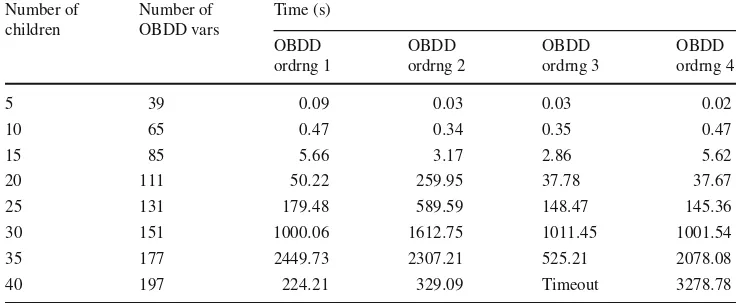
The experimental results for various number of horses are reported in Table3. On this scenario, the OBDD ordering 1 offers the best performance on large models. It is worth point-ing out that the runnpoint-ing time for the model with 40 horses is shorter than that with 35 horses under the first OBDD ordering. This is because the former model has better
struc-G: HML K: hml
0 : 0
G: ML K: ml
0 : 1
H:h
G: HL K: ml 0 : 1
M:h
G: HM K: ml
0 : 1 L:h
G: L K: l 0 : 2
M:m
G: M K: l 0 : 2
L:m
G: L K: l 1 : 1
H:m
G: H K: l 0 : 2 L:m M:m
G: M K: l 1 : 1 H:m
0 : 3 L:l
1 : 2 M:l L:l H:l
[image:16.595.279.543.101.589.2]2 : 1 M:l
Fig. 12 The general’s strategy in the Tian Ji puzzle
tural regularity, which makes the OBDD operations more efficient.
5.2 Applications
[image:16.595.309.541.332.589.2]Table 3 Experimental results
for racing horses Number of children
Number of OBDD vars
Time (s)
OBDD ordrng 1
OBDD ordrng 2
OBDD ordrng 3
OBDD ordrng 4
5 39 0.09 0.03 0.03 0.02
10 65 0.47 0.34 0.35 0.47
15 85 5.66 3.17 2.86 5.62
20 111 50.22 259.95 37.78 37.67
25 131 179.48 589.59 148.47 145.36 30 151 1000.06 1612.75 1011.45 1001.54 35 177 2449.73 2307.21 525.21 2078.08 40 197 224.21 329.09 Timeout 3278.78
5.2.1 Verification of authentication protocols
Authentication protocols are a class of security protocols whereby two or more agents need to acquire knowledge of their identity, typically to initiate secure communication. Authentication protocols are notoriously difficult to analyse, due to the possible existence of subtle bugs such as man-in-the-middle attacks and impersonation. Formal models have been employed to analyse authentication protocols; how-ever, they are often limited to reachability analysis only, thereby imposing rather severe limitations on the class of specifications that can be verified. Specifications concerning authentication are amenable to be expressed in a temporal-epistemic logic language as they concern states of knowledge of the principals in a system.
Authentication protocols expressed in CAPSL, a main-stream language for the description of security protocols, were automatically verified with MCMAS in [5]. Specifi-cally, a compiler was built to translate protocols from the Clark–Jacobs and SPORE repository [62] into MCMAS readable input. This involved devising a translation from the SPORE protocol description into ISPL and a transla-tion from the SPORE protocol specificatransla-tions (“goals” in CAPSL) into appropriate temporal-epistemic formulas. The methodology is completely automatic and was evaluated on well-known key establishment protocols. The tool confirmed bugs already known in some key establishment protocols and verified the correctness of others. Since MCMAS also provides counterexamples when a specification is false, an attack could easily be derived by inspecting the output of the checker.
The performance of the methodology was in line with state-of-the-art model checkers for security protocols. It has been argued, see, e.g. [8,31], that epistemic specifications are considerably more intuitive for the security analyst as they refer precisely to the states of knowledge of the princi-pals, which are the basic primitive in security analysis. This increase in expressiveness allows also the validation of other specifications, including the distributed detection of attacks
at run-time [6]. Lazy intruder models are known to increase the effectiveness of model checking approaches for security protocols [3]; they can also be applied in the context of secu-rity specifications [46].
5.2.2 Verification of anonymity protocols
Anonymity protocols are a class of protocols aimed at estab-lishing the privacy of principals during an exchange. For example, the onion routing protocol can guarantee the com-munication between two parties without their identities being revealed to any third party.