Wide-area mapping of small-scale features in agricultural landscapes using airborne remote sensing

Wide-area mapping of small-scale features in agricultural landscapes

using airborne remote sensing

Jerome O’Connell

, Ute Bradter, Tim G. Benton

School of Biology, Faculty of Biological Sciences, University of Leeds, LS2 9JT, UK

a r t i c l e i n f o

Article history: Received 8 May 2015

Received in revised form 25 July 2015 Accepted 15 September 2015

Keywords: Random forest Object orientated Agriculture Aerial photography Spatial analysis Classification

a b s t r a c t

Natural and semi-natural habitats in agricultural landscapes are likely to come under increasing pressure with the global population set to exceed 9 billion by 2050. These non-cropped habitats are primarily made up of trees, hedgerows and grassy margins and their amount, quality and spatial configuration can have strong implications for the delivery and sustainability of various ecosystem services. In this study high spatial resolution (0.5 m) colour infrared aerial photography (CIR) was used in object based image analysis for the classification of non-cropped habitat in a 10,029 ha area of southeast England. Three classification scenarios were devised using 4 and 9 class scenarios. The machine learning algorithm Random Forest (RF) was used to reduce the number of variables used for each classification scenario by 25.5 % ± 2.7%. Proportion of votes from the 4 class hierarchy was made available to the 9 class scenarios and where the highest ranked variables in all cases. This approach allowed for misclassified parent objects to be correctly classified at a lower level. A single object hierarchy with 4 class proportion of votes produced the best result (kappa 0.909). Validation of the optimum training sample size in RF showed no significant difference between mean internal out-of-bag error and external validation. As an example of the utility of this data, we assessed habitat suitability for a declining farmland bird, the yellowhammer (Emberiza citronella), which requires hedgerows associated with grassy margins. We found that22% of hedgerows were within 200 m of margins with an area >183.31 m2_{. The results from this analysis} can form a key information source at the environmental and policy level in landscape optimisation for food production and ecosystem service sustainability.

Ó2015 The Authors. Published by Elsevier B.V. on behalf of International Society for Photogrammetry and Remote Sensing, Inc. (ISPRS). This is an open access article under the CC BY-NC-ND license ( http://creati-vecommons.org/licenses/by-nc-nd/4.0/).

1. Introduction

Agricultural land covers approx 38% of the earth’s terrestrial surface (FAO, 2014) and therefore plays a key role in biodiversity, conservation and ecosystem service delivery at a variety of spatial scales (Billeter et al., 2008; Tscharntke et al., 2005). However increasing pressures are likely on the fragmented habitats within these landscapes with the global population set to exceed 9 billion by 2050 driving demand that may require a doubling of food pro-duction (Godfray et al., 2010; Tilman et al., 2011). In agricultural landscapes non-cropped habitats are primarily made of features such as trees, hedgerows and grassy margins. For the purpose of this study a margin is a buffer stripP2 m wide and a hedgerow is defined as a length of small trees and shrubsP20 m long and

65 m wide (Maddock, 2008). Trees are defined as having an indi-vidual crown >6 m2_{and may occur within a hedgerow, in isolation}

or as part of a woodland/forest. In the UK the total length of hedge-rows fell from an estimated 800,000 km in 1956 to under 500,000 km in 1994 (Cornulier et al., 2011) to 477,000 km in 2007 (Carey et al., 2008). Recent reforms to the Common Agricultural Policy (CAP) have encouraged farmers to manage such features by means of financial payments through various agri-environmental schemes overseen by the Department for Environment, Food and Rural Affairs (DEFRA) in England. Features such as hedgerows and margins, are protected under UK (DEFRA, 1997, 2004) and EU (EU, 2007) law due to their importance as an ecological network across mono-cultured landscapes with distribution and connectivity having significant effects on land-scape scale biodiversity and regional biota (Benton et al., 2003; Power, 2010). Many ecosystem services depend on the amount, quality and configuration of non-cropped land, as well as the landuse within fields (Benton, 2007; Billeter et al., 2008; Power, 2010). For example, simplification of the landscape through increased field size and reduced natural vegetation cover, especially of grassland areas, has been shown to increase pest

http://dx.doi.org/10.1016/j.isprsjprs.2015.09.007

0924-2716/Ó2015 The Authors. Published by Elsevier B.V. on behalf of International Society for Photogrammetry and Remote Sensing, Inc. (ISPRS). This is an open access article under the CC BY-NC-ND license (http://creativecommons.org/licenses/by-nc-nd/4.0/).

⇑ Corresponding author.

E-mail address:[email protected](J. O’Connell).

Contents lists available atScienceDirect

ISPRS Journal of Photogrammetry and Remote Sensing

damage due to lower populations of natural enemies (Gardiner et al., 2009).

Given the importance of the amount, connectivity, heterogene-ity and qualheterogene-ity of non-cropped habitat for biodiversheterogene-ity and other ecosystem services, spatially extensive knowledge on the location and state of these habitats has now been recognized as a key variable in mapping and modeling ecosystem service delivery and sustainability at local, regional and national scales (Dale and Polasky, 2007; Kremen et al., 2007; Watson et al., 2011). Many of the processes involved need to be assessed at landscape level which makes traditional field based surveys expensive and time consuming.

Remote sensing has long since been used to map biodiversity at a variety of spatial scales (Turner et al., 2003). However non-cropped features in the UK are often below the spatial resolution of many satellite sensors (i.e. <5 m), therefore alternative platforms are required for accurate delineation of their extent (O’Connell et al., 2013a). Some studies have used image fusion to enhance the spatial resolution of multispectral bands (Aksoy et al., 2010) while others have looked at sub-pixel image classification for the detection of small scale woody elements in the landscape (Foschi and Smith, 1997; Thornton et al., 2007). Many other approaches focus on the use of edge detection kernels to detect spectral boundaries which may be indicative of hedgerows or margins in agricultural land-scapes (Fauvel et al., 2012; Rydberg and Borgefors, 2001). All these approaches are pixel based and rely on either high spatial resolution panchromatic data for contrast or multispectral data to classify the features based on spectral response. Other approaches have classi-fied trees, hedge and shrub vegetation by combining multispectral and structural data via stereo imaging (Tansey et al., 2009), Light Detection And Ranging (LiDAR) (Hellesen and Matikainen, 2013) and radar (Scholefield et al., 2012). While these approaches offer robust mapping of tall vegetation, they generally don’t enhance the classification of surface vegetation such as grassy margins, can be costly to acquire and generally are not suitable for regional scale mapping due to low spatial resolution or low spatial coverage.

An alternative approach to the use of pixels is the use of objects which can add additional information to features of interest which can then be utilised in an Object Based Image Analysis (OBIA) protocol (Blaschke, 2010). OBIA uses a variety of spectral, textural, geometric, thematic and contextual attributes built from the aggregation of homogeneous pixels into real world objects, there-fore the size of uncorrelated feature space is significantly increased when compared to traditional pixel based approached (Benz et al., 2004; Mallinis et al., 2008; Myint et al., 2011). Non-cropped fea-tures in structured agricultural landscapes generally have high geometric and contextual properties; e.g. margins typically have a high length-to-width ratio, show a high contrast to neighbouring features such as hedges and are located at the edge of fields. Sev-eral studies have used OBIA in the classification of non-cropped features such as trees and hedges with varying levels of success (Bock et al., 2005; Mueller et al., 2004; Sheeren et al., 2009; Tansey et al., 2009; Vannier and Hubert-Moy, 2008). Classification in OBIA has been dominated by algorithms such as maximum like-lihood, nearest neighbour and Knowledge Based Classifiers (KBC) (Blaschke, 2010). A KBC incorporates expert knowledge in building a set of rules that utilise the attributes of each object in the image and have proved successful in the classification of non-cropped areas in the UK (O’Connell et al., 2013a; Tansey et al., 2009). How-ever the creation of a robust KBC is an iterative process which can be time consuming with respect to the selection of suitable fea-tures and thresholds (Stumpf and Kerle, 2011). Model transferabil-ity can be a significant issue where the thresholds and membership functions within the rule-base break down when the KBC is applied to data which was taken at a different time or location (O’Connell et al., 2013a). An alternative approach which is gaining

popularity within the remote sensing community is the use of machine learning or ensemble algorithms such as Support Vector Machine (SVM) and Random Forest (RF) in OBIA (Duro et al., 2012). Such algorithms have advantages over conventional algo-rithms based on their ability to detect subtle and complex patterns in high dimensional data using robust statistical techniques with a high degree automation (Blaschke, 2010; Rodriguez-Galiano et al., 2012). Previous experience of RF (Breiman, 2001) from some of the authors of this study in the classification of complex habitats in the Yorkshire Dales National Park in the UK (Bradter et al., 2011) gave an indication of its potential when applied to environmental and remote sensing data.

RF is based on an ensemble of decision trees which are each grown on random selections of two thirds of the data with replace-ment. This ‘‘bagging” approach makes the algorithm more insensi-tive to noise in the data (Rodriguez-Galiano et al., 2012), including variations in reflectance due to solar zenith or Biodirectional Reflectance Distribution Function (BRDF) (Chan and Paelinckx, 2008). This concept of machine learning by randomisation over multiple iterations allows for discernible pattern to emerge from highly dimensional data. The set of variables used at each decision node is randomly selected which can reduce the strength of indi-vidual trees but also reduces correlation between trees and thus reduces the generalisation error (Liaw and Wiener, 2002). The pro-portion between misclassifications and the total number of Out Of Bag (OOB) elements (i.e. the remaining one third of data) con-tributes to an unbiased estimate of generalisation error. This error converges as the number of trees increases; therefore adding more trees does not over fit the data (Cutler et al., 2007). RF uses the ‘‘best” variables at each node based on node purity. Several options to calculate variable importance exist, including permutation importance which is calculated by randomly permutating all val-ues in the selected variable and using the difference in OOB error as an indication of the importance of that variable to the classifier. Pruning of trees is not necessary as the final classification is based on the majority vote of all trees within the forest. The package ran-domForest 4.6–7 (Liaw and Wiener, 2002) was used in the R (3.0.1) statistical coding environment (R Development Core Team, 2014), which is based on the original Fortran programs by Breiman and Cutler (https://www.stat.berkeley.edu/~breiman/RandomForests/ cc_software.htm).

The objective of this study was to create a novel and robust clas-sification protocol for the mapping of non-cropped features in a ‘‘case study” agricultural landscape. The protocol needed to be semi-automated to enable wide area mapping of such features with a minimal number of variables. Based on these criteria and results from a previous studies (Bradter et al., 2013; O’Connell et al., 2013a) as well as a review of some comparative studies with other algorithms (Chan and Paelinckx, 2008; Duro et al., 2012; Lawrence et al., 2006; Pal, 2005; Rodriguez-Galiano et al., 2012), it was felt that OBIA with the ensemble classifier RF may yield best results. The combination of both approaches in remote sensing is a relatively new area of research and yields some uncertainties in the areas of optimisation of RF parameters, model transparency, train-ing and validation size, hierarchical accuracy assessment and fea-ture selection/importance with respect to class and object hierarchy. This study addresses some of the aforementioned uncer-tainties through the mapping of non-cropped areas using OBIA and the machine learning classifier RF.

2. Materials

2.1. Study area

arable crops and temperate grassland over a mosaic of lime rich loam, clay loam and sandy soils (NSRI, 2011). The topography of the site was undulating with an elevation range of 22–73 m, mean of 45 m and total area of 10,029 ha. Annual rainfall for the region was 810 mm, with an average of 130 days of rain per year (Met, 2012). Despite being intensively managed, the site contained vari-ous designated areas (Fig. 1) including; 12.4% under the England Habitat Network (Catchpole, 2007), 5.9% under Countryside Ste-wardship/Environmental Stewardship and 0.3% under priority grassland habitat via the UK Biodiversity Action Plan (BAP) (JNCC, 2007).

2.2. Data

An airborne survey of the study area was commissioned for the summer of 2012 and completed on the 6th of September that year. The survey used a Vexcel UltraCam-Xp (Vexcel, 2008) pan-sharpened to 25 cm spatial resolution at an altitude of 4230 m ± 1 m. The data was projected to British National Grid (EPSG: 27700) with level 3 geometric correction and cubic convolution resampling. Landcover and boundary information was acquired from the Ordnance Survey (OS) MasterMap topogra-phy layer (OS, 2010). The topography layer gave information on nine themes; land area classifications, buildings, roads, tracks and paths, rail, water, terrain and height, heritage and antiquities, structures and administrative boundaries at 1:1250 to 1:10000 scale. Accuracy assessment of the various categories (kappa 0.68) from a previous study (O’Connell et al., 2013a) was used to identify themes that gave the most robust representation with respect to this study. Field data was also collected between late June to late August 2012 in the cropped and non-cropped areas. The sampled farms were initially stratified based on soils data (NSRI, 2011), with some constraints imposed due to land access permission. For each farm, a representative sample of vegetation communities present

within the non-cropped areas was made. Homogeneous sections of hedgerow were mapped using a Global Positioning System (GPS) with waypoints at either end. Individual trees were also mapped with a GPS, with tree height and species also included. Crop type in fields was recorded as part of the hedge/tree survey. Additional visual ground-truthing was aided by a July 2008 GeoEye 1 image and commissioned 25 cm aerial photography from June 2014 (ARSF, 2014). Information on designated areas (Fig. 1) were accessed from the Natural England GIS database (NE, 2012).

3. Methods

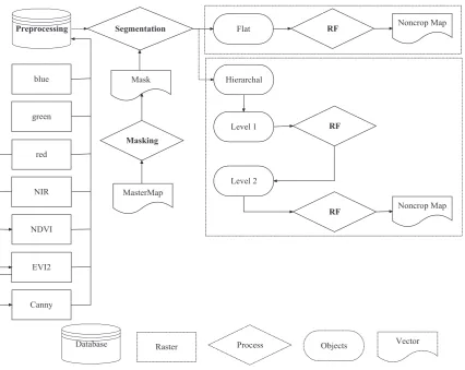
The processing chain for this study was divided up into four key processes (bold inFig. 2), each of which is outlined in the following sections.

3.1. Preprocessing

Fifty-two image tiles (134 tiles) were produced from the air-borne survey; 17,310 pixels across track11,310 pixels along track (pan-sharpened), with a 60% overlap along track and 40% overlap across track. Sub-pixel accuracy image mosaicing and his-togram based colour matching was undertaken using Erdas Imag-ine’s MosaicPro software (Intergraph, 2013). To assist in the classification process the Normalised Difference Vegetation Index (NDVI) (Sellers, 1985) and Enhanced Vegetation Index 2 (EVI2) (Jiang et al., 2008) were calculated. NDVI correlates with vegetation health and vigor (Carlson and Ripley, 1997) and EVI2 has been shown to be more sensitive than traditional indices in highly vegetated landscapes or where soil reflectance can be prominent (Jiang et al., 2008; O’Connell et al., 2013b). The Canny edge-detection algorithm (Canny, 1986) was used on the EVI2 (O’Connell et al., 2013a) image to emphasize boundaries using eCognition software (Trimble, 2013a).

3.2. Masking and class structure

The MasterMap topography layer (OS, 2010) was used to create a mask using landcover categories of known accuracy based on a previous study (O’Connell et al., 2013a). The topography layer was first converted to objects in eCognition on a separate map using the chessboard segmentation algorithm (Trimble, 2013b) and then synchronised with the airborne data on the main process-ing level projected to British National Grid (EPSG: 27700). A simple rule based classifier (Appendix A) using the MasterMap FeatCode, DescTerm and DesGroup attributes (OS, 2010) and a vegetation threshold was used to extract all objects for the predefined classes. The primary classes used, with FeatCode in parentheses, were: Buildings (10021), Manmade (10056), Trees (10111), Mixed (10053) and Water (10086). The area coverage of these classes (6.75% of the study area) was then used as a mask in the segmen-tation of the airborne data on the main processing level (Fig. 2).

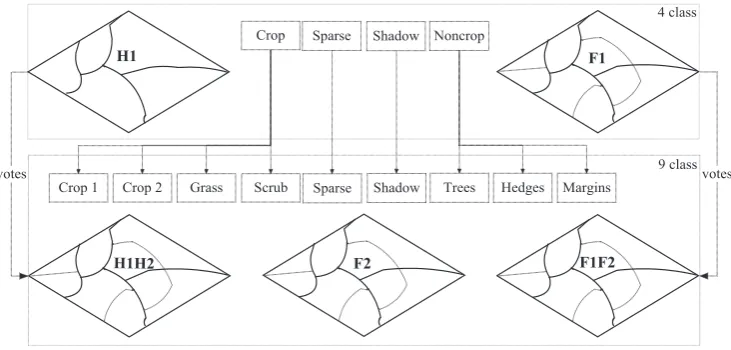
The class structure was based on an initial 30 spectral classes derived from the Iterative Self-Organizing Data algorithm (ISO-DATA) (Ball and Hall, 1965) and landcover information from the field data. A class hierarchy was present for some classification sce-narios (Fig. 3) depending on the segmentation procedure (Sec-tion3.3), however all scenarios where completed using the same final nine class structure. Many of the arable crops were merged to two distinct classes; closed canopy (Crop 1) and open canopy (Crop 2) as the focus was in mapping non-cropped areas. Grass was defined as intensively managed grassland and Scrub charac-terised as having a heterogeneous structure and often occurring in field corners, urban parks or around woodlands. The class Crop (4 class hierarchy) was based on merger of all vegetation classes

that weren’t non-crop (Fig. 3). Sparse vegetation was based on a mean spectral threshold (EVI2 < 45, 8 bit scaled) which was obtained from MasterMap sealed surface classes, field data and visual examination. The Sparse and Shadow classes were present as complete objects all segmentation scenarios (Section 3.3), therefore both classes were included for both the 4 and 9 class sce-narios (Fig. 3).

3.3. Image segmentation

In this study the multiresolution segmentation algorithm (Baatz and Schäpe, 2000) was used in the main segmentation process using eCognition. To segment, we used two approaches; flat (single) and hierarchical (multi-scale) segmentation. Multi-scale segmentation creates a hierarchical object structure based on the premise that real world features are found in an image at different scales of analysis (Blaschke, 2010). The object hierarchy was based on the class structure, with top down approach adopted, to classify cropped objects at larger scale factors (e.g. H1 inFig. 3), thereby focusing the analysis on the smaller objects in the non-cropped areas at lower segmentation scales (e.g. H1H2 inFig. 3).

Optimisation of the scale parameter for both the flat and hierar-chical segmentation used the Estimation of Scale Parameter (ESP 2) tool (Dra˘gutßet al., 2014), which eliminated the subjectivity of ref-erence objects (Witharana and Civco, 2014). For the hierarchical approach the ESP 2 settings were a top down hierarchy with a starting scale and step size of 1 for level 1, 5 and 25 for level 2 and 100 and 25 for level 3 and number of loops set to 400. For the flat approach the starting scale and step size for level 1 was 1, 1 and 10 for level 2 and the number of loops set to 300. The tool

outputs a graph with local variance and rate of change of local vari-ance plotted as a function of scale factor. This was used to cross-reference the retained scale factors by visually examining break points in rate of change curve after continuous decay (Drǎgutß

et al., 2010).

3.4. Classification

3.4.1. Training data

Training data were extrapolated from the field data where mul-tiple points were created from individual non-cropped polygons delineated from GPS waypoints and crop varieties in fields. This extrapolation of field data labelled 5.59% (4799) of the total popu-lation of objects for the hierarchical and 3.22% (5713) for the flat scenario. Previous studies have shown that classifiers like RF tend to produce higher accuracies for majority over minority classes (Chen et al., 2004; Lin and Chen, 2012) and show greater variability in variable importance values as a result of class imbalance (Janitza et al., 2013). The 4 class objects in this study were therefore resam-pled to615% of the smallest sample size (i.e. Shadow) to maintain a sufficient level of class balance. With the increased use of machine learning algorithms in remote sensing there has been lit-tle reporting of the influence of training data size on classification accuracy. It has also been reported that RF does not need external validation due to the prediction accuracy calculated using the OOB sample (Breiman, 2001). However the robustness of this calcula-tion is based on several assumpcalcula-tions, one of which is the size of training sets and subsequent OOB sample sizes. In this study we compared the error rates between the internal (OOB error) and external validation. A total sample size of 5713 objects was used with 30% of the data used for external validation. Training data were sampled randomly from the remaining 70% for the external validation and from the full dataset for the internal validation. Training data size was varied between 10% and 70% in steps of 10% with external and internal (OOB) error rates calculated. Valida-tion was repeated 10 times for each training data size using a new random sample (for the 70% size of the external validation all remaining points were used). Error rates for the internal and exter-nal validation were compared using a generalised linear squares (GLS) model. In the GLS model different variances per factor level were allowed (likelihood ratio test between model with and with-out allowing for different variances per stratum:L= 37.0,df= 13,

p= 0.0004), with sample size fitted as a fixed factor. Error stabilisa-tion as a funcstabilisa-tion of sample size was also investigated for the OOB error to see if an asymptote would be reached with respect to

increasing sample size. Again 10 random samples per size category were used (10–100% in steps of 10%), with a GLS model allowing for different variances per sample size (likelihood ratio test between model with and without allowing for different variances per stratum: L= 72.4,df= 9, p< 0.0001). Differences between different levels of the factor sample size were explored using contrasts.

3.4.2. Variable selection

Once the segmentation process was completed object variables (i.e. features) were calculated for each level in each scenario. The eCognition software offers a significant array of object based vari-ables. However many of these variables are highly correlated and while RF has been shown to deal well with correlated predictors (Chan and Paelinckx, 2008; Gislason et al., 2006), the additional computational effort required to process them is inefficient for a large scale mapping protocol. Therefore a variable selection pro-cess was used (Genuer et al., 2010) which selected variables based on ranked mean importance as a function of OOB error. The func-tion used (Bradter, 2013) was written in R using the parameters;

ntree: 2000, mtry: square root of the number of variables with the result averaged over 50 repetitions (Genuer et al., 2010).

The variables used were divided up into 5 main categories (spectral, geometric, neighbourhood, textural and thematic) with the total number of variables changing for each classification sce-nario (Fig. 3b). Spectral referred to variables that were derived directly from the 6 spectral images and the Canny image. Geomet-ric variables were based on within object geometGeomet-ric properties (e.g. length/width) and ratio based properties (e.g. area to super object). Neighbourhood variables were derived from spectral and textural ratios, constrained by a distance or object count window. Texture variables were calculated after Haralick analysis (Haralick et al., 1973) and based in all directions for directional invariance (Trimble, 2013b). Thematic variables were based on the FeatCode attribute from neighbouring and parent objects as well as propor-tion of votes from the 4 class models (see Secpropor-tion3.4.3).

3.4.3. Random forest

All RF models were run using the package randomForest (Liaw and Wiener, 2002) in R 3.0.1 (R Development Core Team, 2014). Predictions using the selected variables were made using the fol-lowing parameters: 50 iterations,ntreeset to 500, proximity and importance set to true (importance based on mean decrease in accuracy) and all remaining parameters as default. The mtry

parameter was varied between 1 and 15 to assess its effect on

OOB error. The proportion of votes was used instead of the major-ity prediction as a variable for the 9 class scenarios. This gave a bet-ter indication of the confidence of the 4 class result rather than a single categorical value which would have resulted from a majority vote. This ‘‘soft” class hierarchy methodology is ideally suited to RF as it allows for discernible patterns to emerge at each level without error propagation due to local classifiers. Classification accuracy was assessed using both flat and hierarchical measures. The flat approach used overall, user, producer and kappa measures (Congalton and Green, 2008) which were derived from a confusion matrix generated from the OOB data using the R package Caret (6.0–37) (Kuhn, 2015). Hierarchical assessment differs from tradi-tional approaches in that it encompasses the multi-level class structure in the final estimation of accuracy. The hierarchical assessment in this study was based on the hierarchical F measure described byKiritchenko et al. (2005)and recommended bySilla and Freitas (2011). In short (seeAppendix Bfor more detail), the measure extends the regular precision, recall and F measures by accounting for the location of each observed and predicted class of each case (object) in the class hierarchy (Fig. 3).

Once completed, randomForest classification results were exported into the eCognition software where the MasterMap masked classes (i.e. Buildings, Manmade, Trees, Mixed and Water) were segmented using the same scale factors as the classification scenarios. A k-Nearest-Neighbour (kNN = 1) classifier was built for each MasterMap class using all the objects classified in the RF model as training data. Post-classification, various morphological processes (e.g. growing and shrinking) were used to adjust class boundaries as previous work had shown the MasterMap data to have poor delineation of many natural and manmade features (O’Connell et al., 2013a). A simple set of rule base classifiers were also created to remove individual errors; e.g. ‘‘classify Crop 2 as Trees if the object is completely enclosed by Trees, <55 pixels and are ±0.0125 EVI2 of the mean of the class Trees”. A random sample of 450 objects was selected from the kNN classification to assess its accuracy based on the RF training data.

3.4.4. Spatial analysis

To explore the utility of the classification map, we assessed the spatial distribution of non-cropped features within the study area. Spatial clustering was assessed in ArcGIS (ESRI, 2012) using nearest neighbour analysis on margins and hedgerows, based on euclidean distance across the whole study site for both classes. To examine the degree of spatial clustering as a function of area, incremental spatial autocorrelation (Moran’s I) was used on margins and hedgerows over 15 stages at increments of 30 m starting at 300 m. Habitat fragmentation was assessed for hedgerows and margins using 6 categories of fragmentation (interior, perforated, edge, transitional, patch, and undetermined) as outlined by Riitters et al. (2000). This was done using the geoscientific software SAGA (SAGA, 2015) and the add-on package Module Fragmentation (Conrad, 2008) with a maximum and minimum neighbourhood setting of 10 and 3 respectively. To provide a specific focus, we used the map to identify potential nesting habitat (seeAppendix D) for the bird species Emberiza citronella (Yellowhammer). The criteria were to identify large areas of margin that were in close proximity to long lengths of hedgerow (Douglas et al., 2010; Morris et al., 2001).

4. Results

4.1. Image segmentation

ESP 2 analysis identified a scale parameter of 295 for H1 giving 19,880 objects and a scale parameter of 110 for H2 giving 858,49

objects (Fig. 3). For the flat approach a single scale parameter of 96 was selected from a possible three (i.e. 422, 256, 96) giving 177,419 objects.

4.2. Training sample size

For training sample size the interquartile range within each sample size decreased with increasing sample size (Fig. 4).

There was no significant difference found in the OOB error rate between sample sizes of 90% and 100% (parameter estimate:

0.0014 ± 0.0007, p= 0.0632) and differences between sample sizes of 80% and 90% were already very small (parameter estimate:

0.0024 ± 0.0010, p= 0.025). For training sample size the mean error rates from the internal OOB validation were not significantly different to those from the external validation with Likelihood ratio value (L) of 1.06 (p-value = 0.304) (Zuur et al., 2009).

4.3. Variable selection

Results from themtryparameter tests showed little variation in OOB error (±0.0025) when varyingmtry. For this reasonmtrywas set to the square root of the total number of variables which is the default setting for classification in randomForest (Liaw and Wiener, 2002).

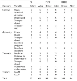
A total of 90 variables for the F2, 94 for the F1F2 and 108 vari-ables for the H1H2 model (Appendix C) were created in eCognition. Variable selection (Bradter, 2013) reduced the number of variables by 25.5% ± 2.7% for the three models; 27.8% for the F2 model, 26.6% for F1F2 and 22.2% for the H1H2 model (seeAppendix Cfor more detail).

4.4. Classification

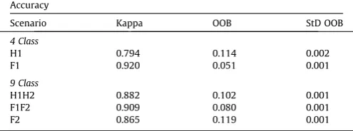
Variable importance showed some similarities across the 3 classification models when proportion of votes are excluded (Table 1). Classification accuracy for the H1 and F1 models was a kappa value of 0.794 and 0.920 respectively (Table 2). The model F2 performed poorest for the 9 class scenario with F1F2 performing best indicating the importance of the 4 class propor-tion of votes as this was the only difference between the two models. Overall accuracy for F1F2 was also very high (Table 3) with a precision, recall and f-measure of 0.959 which compares very favorably with other non-cropped mapping studies (Aksoy et al., 2010; Rydberg and Borgefors, 2001; Sheeren et al., 2009; Tansey et al., 2009).

4.5. Spatial statistics

(55.47%), with the edge category at 21.43%. The declining farmland bird, the Yellowhammer, prefers nesting in hedgerows and foraging for its young in margins within 200 m of the nest site (Douglas et al., 2010, 2009). Based on these criteria 9.35% of the total population of hedgerows were within 25 m of areas of margin that were >183.31 m2 _{(Table 4). A cumulative total of 21.53%}

(40.21 ha) of all hedgerows were within 200 m of large margins areas (Appendix D).

5. Discussion

The selected scale parameter for image segmentation was cho-sen as it gave the best delineation of the target features trees, hedgerows and margins. The increased number of objects for the flat hierarchy was due to the absence of any connection to larger scale parent objects (i.e. H1). Results from the analysis of training sample size showed that the OOB error provided a similar accuracy measure to the mean overall error from an external validation. This stabilisation of mean error rate indicates that, with the full training dataset, the training data was representative for the study area.

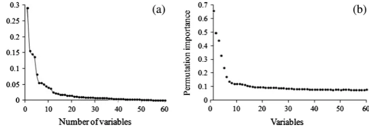
By plotting mean class and overall error based on 50 RF models, there was a clear trend of error stabilisation above 100 trees for all classification scenarios, validating the ntree parameter, as RF does not induce an over adjustment in the model above the convergence point (Breiman, 2001). Variable selection was not performed on the 4 class models (i.e. F1, H1) due to the lower number of variables produced at this level and considering that only the proportion of votes from this level were inputted into two of the 9 class mod-els. Class specific variable importance also showed clear trends with Sparse, Shadow, Grass, Crop 1 and Crop 2 dominated by spec-tral and textural features and Scrub, Trees, Hedges and Margins dominated by spectral and geometric features (Table 1). The dis-tinction between Grass and Scrub was predominantly driven by textural and geometric variables with Scrub having higher stan-dard deviation in GLCM and lower area. For H1H2 and F1F2, the top ranked variable for 7 of the 9 classes was proportion of votes, with the 4 class vote correctly attributed to the 9 class category (i.e. Noncrop for Trees) in all cases. A trend of significant decrease in permutation importance for the first ten ranked variables was present for all three models (Fig. 5b). Variables from 20 and above had little influence on classification accuracy as mean OOB error was stabilised (Fig. 5a).

Lower user and producer accuracy for Hedges was evident as there was some commission and omission with Margins and Trees. All three non-cropped classes were often in a similar spatial and spectral domain with similarly ranked variables; therefore it was unsurprising that some confusion did exist. Scrub, while having high user and producer accuracy, did have some confusion with Crop 1, Crop 2 and Grass. This was due to the fact that the Scrub class transcended many spectral textural, geometric and thematic variables and therefore in some occasions didn’t have a key set of variables that best defined its class description. Crop 2 had minor confusion with Scrub and this was attributed to a high mean and standard deviation in GLCM which was characteristic of both classes. It’s likely that the confusion in this study between the cropped classes would have been significantly reduced by the inclusion of additional images taken throughout the growing season. In this case the different management practices for the

Fig. 4.Box plots showing External (a) and Internal (OOB) (b) error as a function of sample size over 10 repetitions; where P10 is 10% sample size, P20 is 20% sample size etc. Whiskers represent the max and min, top and bottom of the box plot by 3rd and 1st quartile and the median by the centreline. TheYaxis applies to both plots.

Table 1

The top 15 variable importance rankings across all 9 classes for the 3 different classification models (i.e. F2, F1F2 and H1H2). Superscript letters indicate variable category. SeeAppendix Cfor more details.

Rank F2 F1F2 H1H2

1 GLCM_Dissid

Crope

Crope

2 Mean_Vis1a

Noncrope

GLCM_Dissid

3 Mean_Vis3a

Sparsee

Noncrope

4 GLCM_Corred

GLCM_Dis_1d

GLCM_Corred

5 Mean_Vis2a _{Mean_Vis3}a _{Ratio_NDVI}a

6 Length/Widthb

Length/Widthb

Asymmetryb

7 Asymmetryb

GLCM_Corred

Mean_Vis3a

8 GLCM_Mean_d

Mean_Vis1a

Mean_Vis2a

9 Border lengthb

Mean_Vis2a

Circular_Mb

10 FeatCodee

Asymmetryb

Mean_Vis1a

11 Edge_Contrc

Shadowe

Ratio_EVI2a

12 StD NIRa _{GLCM_Mean_}d _Brightnessa

13 Diff to Cannya

StD NIRa

GLCM_Ang_2d

14 Mean_EVI2a

Dist to Sparsec

GLCM_Mean_d

15 StD Vis3a

HSI_Transfa

Dist to borderc

16 Diff to EVI2a

Length mb

HSI Transfa

17 Mean NDVIa

GLCM_Ang_2d

Dist to Mixedc

18 Mean NIRa _{GLCM Entro}d _Sparsee

19 HSI Transfa _{Mean_EVI2}a _{StD NIR}a

20 Area m2b

Diff to Cannya

FeatCodee

a

Spectral.

b

Geometry.

c

Neighbourhood.

d

Texture.

e _Thematic.

Table 2

Kappa, OOB error and standard deviation in OOB (StD OOB) error (based on 50 forests) for all 4 and 9 class models.

Accuracy

Scenario Kappa OOB StD OOB

4 Class

H1 0.794 0.114 0.002

F1 0.920 0.051 0.001

9 Class

H1H2 0.882 0.102 0.001

F1F2 0.909 0.080 0.001

different crops and their associated variation in spectral response would increase the discrimination between classes.

Various studies have demonstrated the benefits of a multi-level object hierarchy in landcover classification (Benz et al., 2004; Blaschke, 2010; Lucas et al., 2007; Mallinis et al., 2008), with parent objects representing general landuse categories and child objects representing more specialised classes. However in this study a single object level with a multi class hierarchy gave the highest overall classification accuracy. This was attributed to the fact that the smaller objects for the F1F2 model were well defined for both the 4 and 9 class scenarios through the large number of spectral, textural, geometric and thematic variables. Some objects for the H1 model may have had both cropped and non-cropped features as signified by the low kappa value. These mixed objects would have had a negative effect on the accuracy of the proportion of votes for the subsequent H1H2 model, reducing its variable importance as a result. Because the unit area for the F1 and F1F2 models were the same, the high kappa value for F1 was directly transferred to the F1F2 model via the proportion of votes resulting in higher importance values for these variables.

Spatial analysis of the non-cropped map showed that although there was significant spatial clustering for margins, this clustering has no correlation with margin size. For hedgerows the autocorrelation with area is at a landscape scale which may have implications for various bird species that depend on the proximity of large clusters of hedgerows. The high percentage of hedgerow in the patch category (fragmentation analysis) was indicative of the discontinuous nature of their distribution as indicated by the nearest neighbour analysis, occurring in small clumps rather than as continuous linear features across the landscape. The increase in the edge category for margins was attributed to the location of the margins relative to other classes in the study area, where the margins typically delineated a transition between crop and non-cropped areas. The analysis of Yellowhammer nesting characteristics indicates the potential predictive utility of this classification approach by identifying algorithmically suitable nesting areas of a red listed bird species (Baillie et al., 2014).

The classification protocol outlined in this study is potentially scalable over large areas of the UK due to the availability of high resolution CIR aerial photography (Landmap, 2014) and the semi-automated fashion of the methodology. While previous studies have demonstrated the potential of mapping hedgerows using various different techniques (Aksoy et al., 2010; Foschi and Smith, 1997; Sheeren et al., 2009; Tansey et al., 2009; Vannier and Hubert-Moy, 2008), the protocol outlined in this study can also identify field margins and scrub areas that are separate to hedgerows and are therefore vital to ecosystem services like pollination. The enhanced spatial resolution of this approach over traditional mapping protocols in the UK (CEH, 2007) is key in assessing small scale habitat features across large

Table 3

Error matrix and accuracy measure for the F1F2 model showing overall, user, producer, kappa, precision, recall and F-measure values.

Sparse Grass Crop 1 Crop 2 Scrub Trees Hedges Margins Shadow Total User

Sparse 755 0 0 0 0 0 0 0 0 755 100.00

Grass 0 471 2 5 21 0 0 0 0 499 94.39

Crop 1 5 13 697 6 11 0 0 0 0 732 95.22

Crop 2 0 10 2 906 26 0 0 0 0 944 95.97

Scrub 0 21 4 35 724 0 0 0 0 784 92.35

Trees 0 0 0 0 0 459 44 13 0 516 88.95

Hedges 0 0 0 0 0 63 459 73 0 595 77.14

Margins 1 0 0 0 0 12 92 476 0 581 81.93

Shadow 0 0 0 0 0 0 0 0 307 307 100.00

Total 761 515 705 952 782 534 595 562 307 5713

Producer 99.21 91.46 98.87 95.17 92.58 85.96 77.14 84.70 100.00

Overall Kappa Precision Recall F-meas

91.97 0.9087 0.9593 0.9593 0.9593

Table 4

Percentage area relative to total area and area (ha) for hedgerows based on their intersection with multiple ring buffers (m) around margin hotspot areas.

Distance 25 50 100 200 300 400 500

% area 0.77 0.57 1.41 2.78 3.06 3.68 1.99

Area (ha) 1.45 1.07 2.63 5.20 5.71 6.87 3.72

landscapes. While the inclusion of datasets derived from active sensors like LiDAR or radar would increase classification accuracy, the coverage of such datasets is still quite limited and this study has demonstrated a very high level of classification accuracy without the need for such data.

Wide area mapping and monitoring of non-cropped areas in the UK could form a key information source at the environmen-tal and policy level with the development of model-based decision, or discussion, tools to optimise landscapes for multiple ecosystem service delivery functions. Knowledge of the characteristics of the non-cropped areas, which is a habitat for a considerable proportion of farmland biodiversity, can be an initial proxy for many difficult-to-assess ecological factors in the landscape – such as natural pest control and pollination services, as well as biodiversity. By simulating landscapes based

on marginal changes on the existing non-cropped areas, it would be possible to find interventions – such as the best sitting and types of agri-environment schemes that have the biggest impacts. As there are increasing calls to manage ecosystem services at the landscape scale (Benton, 2012; Gonthier et al., 2014; Tscharntke et al., 2012), it is necessary to develop tools that are evidence-based but feasible to parameterize from a cost perspective. This study provides some of the methodology which would allow such models to be developed. Such models would aid UK and EU policy goals for the creation of sustainable, multifunctional agricultural landscapes as well as help enable sustainable intensification: increasing the production farmland whilst reducing the impact on the environment. Further work is needed on the spatial and temporal transferability of RF models in the mapping of non-cropped features before a robust tool can be validated for wide area mapping. The inclusion of a temporal stack of imagery will also be investigated as it is likely to significantly aid in the dissemination between the various cropped and margin areas.

6. Conclusions

In this study the integration of the machine learning algo-rithm RF in an object orientated environment was investigated under three classification scenarios. A flat approach signified by a single object hierarchy and 4–9 class structure gave the highest overall accuracy. Parameterisation of RF models was straightforward with mtryvalues greater than 1 producing opti-mal results. Variable importance analysis showed that propor-tion of votes followed by spectral and textural variables were deemed most important for classification accuracy. The inclu-sion of the proportion of votes was a novel approach to trans-ferring class hierarchical information from one level to another and had a significant influence on overall classification accuracy. Analysis of training sample size showed no significant differ-ence between mean internal OOB error and external validation. The classification protocol outlined in this study offers a robust methodology for mapping of cropped and non-cropped areas where high resolution imagery is available. The protocol also allows for the integration of existing land-cover and auxiliary datasets where available, however the inclu-sion of such data is not deemed critical to overall accuracy. The study has shown the potential of machine-learning to correctly classify fine scale ecological features to a high accuracy (on par with field surveys) at a wide spatial extent. The use of such a protocol for mapping and monitoring of cropped and non-cropped areas at local and regional scales could provide a key information source at the environmental and policy level in landscape optimisation for food production and ecosystem ser-vice sustainability.

Acknowledgments

The authors wish to acknowledge the Nigel Bertram Charitable Trust and the Biotechnology and Biological Sciences Research Council (BBSRC) for funding this study. The authors also wish to acknowledge Ordnance Survey UK for access to the MasterMap topography dataset. The authors also like to express their gratitude to the field data collection undertaken by Richard Ellis, Alex Prendergast and Ceirios Davies.

Appendix A

Rule set documentation created in eCognition for the construc-tion of the MasterMap mask. Class definiconstruc-tions are provided in both the Classes and Process Main sections below. Class names are in

italics

Classes: Buildings Manmade Mixed Non Veg

and (min)

[0–60]: Mean EVI2

Scrub

and (min)

Threshold: FeatCode: MasterMap = 10111 Threshold: Mean EVI2 > 100

or (max)

Threshold: DescTerm: MasterMap = ‘‘Rough Grassland”

Threshold: DescTerm: MasterMap = ‘‘Rough Grassland,Scrub”

Threshold: DescTerm: MasterMap = ‘‘Scrub” Threshold: DescTerm: MasterMap = ‘‘Scrub,Rough Grassland”

Small Objects and (min)

Threshold: Area <= 35 m2

or (max)

Threshold: Border toWater>= 1 Pxl Threshold: Border toTrees>= 1 Pxl Threshold: Border toScrub>= 1 Pxl Threshold: Border toNon Veg>= 1 Pxl Threshold: Border toMixed>= 1 Pxl Threshold: Border toBuildings>= 1 Pxl Threshold: Border toManmade>= 1 Pxl

Trees

and (min) or (max)

Threshold: DescTerm: MasterMap = ‘‘Heath” Threshold: DescTerm: MasterMap <> ‘‘Scrub,Rough Grassland”

Threshold: DescTerm: MasterMap <> ‘‘Scrub” Threshold: DescTerm: MasterMap <> ‘‘Rough Grassland,Scrub”

Threshold: DescTerm: MasterMap <> ‘‘Rough Grassland”

Threshold: DescTerm: MasterMap = ‘‘Scrub, Nonconiferous Trees”

Threshold: FeatCode: MasterMap = 10111

Water

and (min)

Threshold: Mean EVI2 <= 100

Threshold: Theme: MasterMap = ‘‘Water” Threshold: FeatCode: MasterMap = 10089

Process: Main:

1. MasterMap extraction

copy map: on main : copy map to ‘MasterMap’. Extraction chessboard

segmentation: on MasterMap : chess board: 99999999 creating ‘Level 1’

2. classification: on MasterMap unclassified at Level 1:

Trees assign class: on MasterMap unclassified with Theme: MasterMap = ‘‘Buildings” at Level 1:Buildings

3. assign class: on MasterMap unclassified with Make: MasterMap = ‘‘Manmade” and DescGroup: MasterMap = ‘‘General Surface” at Level 1:Manmade

4. assign class: on MasterMap unclassified with FeatCode: MasterMap = 10053 and DescTerm: MasterMap = ‘‘Multi Surface” at Level 1:Mixed

5. classification: on MasterMap unclassified at Level 1:

Water

6. classification: on MasterMap unclassified at Level 1:

Scrub

7. edge extraction canny: on main : edge extraction canny (Canny’s Algorithm) ‘EVI2’ => ‘Canny’

Segmentation Level 1

multiresolution segmentation: 108 [shape:0.1 compct.:0.5] creating ‘Level 1’

synchronize map: on MasterMap Buildings,Manmade, Mixed, Scrub, Trees, Water

at Level 1: synchronize map ‘main’

classification: on main unclassified at Level 1: Non Veg classification: unclassified at Level 1: Small Objects remove objects: Small Objects at Level 1: remove objects intoBuildings,

Manmade, Mixed, Non Veg, Scrub, Trees, Water(merge by color)

Appendix B

For the hierarchical accuracy assessment each case contributes to the accuracy measure by the number of nodes found common to the two paths from the observed and predicted classes to the root of the class hierarchy. In this study we re-structured the formula presented byKiritchenko et al. (2005)such that the hierarchical precision, recall andFmeasures (hP,hRandhFrespectively) can be estimated directly from the confusion matrix:

hP¼X

j X

k

ðSj;kFj;kÞ ,

X

k

ðSk;kFþ;kÞ ð1Þ

hR¼X

j X

k

ðSj;kFj;kÞ ,

X

j

ðSj;jFj;þÞ ð2Þ

hF¼ ½ðb2_{þ1Þ hPhR=ðb}2_{hPþhRÞ ð3Þ}

wherej, andkare the observed and predicted classes (rows and col-umns of the confusion matrix),Sj,kthe length of the path from the

first common ancestor of the observed and predicted classesjand

kto the root of the class hierarchy,Fj,kthe number of cases observed

as classjthat were classified as classk,F+,kthe total number of cases

observed as classjandFj,+the number of cases classified as classk.

We further developed terms for thehP,hR andhFfor each class wherebis a weighting parameters (bP0) that controls the relative weight ofhPandhRin the estimation ofhF, with values close to 0 giving more weight tohPand values above 1 giving higher weight tohR. Forb= 1, the harmonic mean ofhPandhFis returned.

Appendix C

for both flat and hierarchical models with the Canny edge image eliminated in all cases. GLCM (Gray-Level Co-Occurrence Matrix) texture variables were retained for all models with all GLDV variables removed. Spearman rho values were high (>0.92) between GLDV (Grey Level Difference Vector) variables and since GLDV is the sum of the diagonals of GLCM it is not surprising that all features were not retained. Just over half the fourteen parent/child (To super object, Table C1) variables were retained for the H1H2 model. All MasterMap landcover

information (Thematic: To super object, Table C1) at level 1 for H1H2 were eliminated for level 2 indicating that there was little correlation between these landuse categories at a level 1 mapping unit. However at level 2 the FeatCode attribute of MasterMap (Thematic: MasterMap, Table C1) was retained for all models with an importance ranking of 10 for F2, 24 for F1F2 and 21 for H1H2 (Table 1). The higher ranking in the F2 model was attributed to the absence of 4 class proportion of votes. The difference in importance of the FeatCode variable between level 1 and 2 was explained by the difference in scale as the level 1 objects often encompassed more than one FeatCode value. The top 20 ranked variables were dominated by textural, spectral and geometric features for all three models; with proportion of votes ranked highest for both the F1F2 and H1H2 models (Table 1). There was little overlap in variables but some overlap in variable categories, especially between F1F2 and H1H2 (Table 1).

Appendix D

The assessment of potential habitat for theEmberiza citronella

(Yellowhammer) was outlined as large margin areas that were within 400 m of areas of significant hedgerow length. The assessment began with hot spot analysis (Getis-Ord Gi) which was performed on hedgerow and margin classes in ArcMap (ESRI, 2012). The assessment for margins was based on area (m2_{) and for hedgerows it was based on length (m). The analysis}

used an inverse distance spatial relationship based on euclidean distance and a threshold distance for analysis which was set to zero to ensure that every feature had a nearest neighbour. After the hotspot analysis margin and hedgerow areas were extracted if they were > mean + 1.5 standard deviations. For margins this meant areas > 183.31 m2_{(mean = 2875.82 m}2_{) and for hedgerows}

this mean lengths > 25.35 m (mean = 787.56 m). This ensured that on the largest margins and longest hedgerows were selected for the final habitat assessment. The resulting margin areas had a multiple ring buffer (25, 50, 100, 200, 300 and 400 m) applied which was used to clip hedgerow areas that satisfied the hotspot analysis threshold (i.e. >25.35 m). The final dataset (Fig. D1) therefore had clusters of margins with large areas and clusters of hedgerows that were between 25 and 400 m from such margins.

Table C1

Object variables used for F2, F1F2 and H1H2 classifiers before and after variable selection. Note the variables under the Thematic category consist of MasterMap categories (i.e. FeatCode) and 4 class proportion of votes from level 1 (e.g. Crop). All variables in the flat classifier are also included in the hierarchical classifier before variable selection with additional variables for the hierarchical classifier due to parent/child features. Other variable names are abbreviated in accordance with eCognition; see the eCognition reference manual for more details (Trimble, 2013b).

F2 F1F2 H1H2

Category Variable Before After Before After Before After

Spectral Mean 7 6 7 6 7 6

Standard deviation

7 6 7 6 7 7

Pixel based 7 6 7 6 7 6

To super object

0 0 0 0 5 5

To scene 5 3 5 3 5 4

HSI 3 1 3 1 3 1

Geometry Extent 6 4 6 4 6 5

Shape 5 5 5 5 5 5

To super object

0 0 0 0 4 3

Based on polygons

5 3 5 3 5 3

Based on skeletons

5 3 5 3 5 4

Thematic Border to 9 5 9 5 9 7

Distance to 9 7 9 7 9 7

Difference to 9 6 9 6 9 7

To super object

0 0 0 0 5 0

MasterMap 1 1 1 1 1 1

4 class votes 0 0 4 4 4 4

Texture GLCM 9 9 9 9 9 9

GLDV 3 0 3 0 3 0

Total 90 65 94 69 108 84

Appendix E. Supplementary material

Supplementary data associated with this article can be found, in the online version, athttp://dx.doi.org/10.1016/j.isprsjprs.2015.09. 007. These data include Google maps of the most important areas described in this article.

References

Aksoy, S., Akçay, H.G., Wassenaar, T., 2010. Automatic mapping of linear woody vegetation features in agricultural landscapes using very high resolution imagery. Geosci. Rem. Sens., IEEE Trans. 48, 511–522.

ARSF, 2014. RC-10 Analogue Camera. NERC, Airborne Research & Survey Facility. Baatz, M., Schäpe, A., 2000. Multiresolution segmentation: an optimization

approach for high quality multi-scale image segmentation. Angew. Geogr. Informationsverarbeitung 12, 12–23.

Baillie, S., Marchant, J., Leech, D., Massimino, D., Eglington, S., Johnston, A., Noble, D., Barimore, C., Kew, A., Downie, I., 2014. BirdTrends 2012: Trends in Numbers, Breeding Success and Survival for UK Breeding Birds. BTO Research Report 644.

Ball, G.H., Hall, D.J., 1965. ISODATA, A Novel Method of Data Analysis and Pattern Classification. Stanford Research Institute, p. 76.

Benton, T.G., 2007. Ecology. Managing farming’s footprint on biodiversity. Science 315, 341–342.

Benton, T.G., 2012. Managing agricultural landscapes for multiple services: the policy challenge. Int. Agric. Policy 1, 7–18.

Benton, T.G., Vickery, J.A., Wilson, J.D., 2003. Farmland biodiversity: is habitat heterogeneity the key? Trends Ecol. Evol. 18, 182–188.

Benz, U.C., Hofmann, P., Willhauck, G., Lingenfelder, I., Heynen, M., 2004. Multi-resolution, object-oriented fuzzy analysis of remote sensing data for GIS-ready

information. ISPRS J. Photogramm. Rem. Sens. 58, 239–258.

Billeter, R., Liira, J., Bailey, D., Bugter, R., Arens, P., Augenstein, I., Aviron, S., Baudry, J., Bukacek, R., Burel, F., 2008. Indicators for biodiversity in agricultural landscapes: a pan-European study. J. Appl. Ecol. 45, 141–150.

Blaschke, T., 2010. Object based image analysis for remote sensing. ISPRS J.

Photogramm. Rem. Sens. 65, 2–16.

Bock, M., Xofis, P., Mitchley, J., Rossner, G., Wissen, M., 2005. Object-oriented methods for habitat mapping at multiple scales‑‘Case studies from Northern

Germany and Wye Downs, UK. J. Nature Conserv. 13, 75–89.

Bradter, U., 2013. Feature reduction following Genuer et al. 2010, 1.0 ed. Unpublished.

Bradter, U., Kunin, W.E., Altringham, J.D., Thom, T.J., Benton, T.G., 2013. Identifying appropriate spatial scales of predictors in species distribution models with the random forest algorithm. Methods Ecol. Evol. 4, 167–174.

Bradter, U., Thom, T.J., Altringham, J.D., Kunin, W.E., Benton, T.G., 2011. Prediction of National Vegetation Classification communities in the British uplands using environmental data at multiple spatial scales, aerial images and the classifier random forest. J. Appl. Ecol. 48, 1057–1065.

Breiman, L., 2001. Random forests. Machine Learning 45, 5–32.

Canny, J., 1986. A computational approach to edge detection. Pattern Anal. Machine Intel., IEEE Trans. 8, 679–698.

Carey, P., Wallis, S., Chamberlain, P., Cooper, A., Emmett, B., Maskell, L., McCann, T., Murphy, J., Norton, L., Reynolds, B., 2008. Countryside Survey: UK Results from 2007. CEH.

Carlson, T.N., Ripley, D.A., 1997. On the relation between NDVI, fractional vegetation cover, and leaf area index. Rem. Sens. Environ. 62, 241–252.

Catchpole, R., 2007. England Habitat Network: Briefing Note. In: England, N. (Ed.). CEH, 2007. Landcover Map 2007. In: Hydrology, C.f.E. (Ed.), Countryside Survey. Chan, J.C.-W., Paelinckx, D., 2008. Evaluation of Random Forest and Adaboost

tree-based ensemble classification and spectral band selection for ecotope mapping

using airborne hyperspectral imagery. Rem. Sens. Environ. 112, 2999–3011.

Chen, C., Liaw, A., Breiman, L., 2004. Using Random Forest to Learn Imbalanced Data. Statistics Department, University of California at Berkeley.

Congalton, R.G., Green, K., 2008. Assessing the Accuracy of Remotely Sensed Data: Principles and Practices. CRC Press.

Conrad, O., 2008. Module Fragmentation (Standard). In: Conrad, O. (Ed.). Cornulier, T., Robinson, R.A., Elston, D., Lambin, X., Sutherland, W.J., Benton, T.G.,

2011. Bayesian reconstitution of environmental change from disparate historical records: hedgerow loss and farmland bird declines. Methods Ecol. Evol. 2, 86–94.

Cutler, D.R., Edwards Jr., T.C., Beard, K.H., Cutler, A., Hess, K.T., Gibson, J., Lawler, J.J., 2007. Random forests for classification in ecology. Ecology 88,

2783–2792.

Dale, V.H., Polasky, S., 2007. Measures of the effects of agricultural practices on ecosystem services. Ecol. Econ. 64, 286–296.

DEFRA, 1997. The Hedgerows Regulations, p. 1160.http://www.legislation.gov.uk/

uksi/1997/1160/contents/made.

DEFRA, R.a., 2004. Single payment scheme: cross compliance handbook for England. In: Rural Payments Agency and Department for Environment, F.a.R.A. (Ed.), London.

Douglas, D.J., Benton, T.G., Vickery, J.A., 2010. Contrasting patch selection of breeding Yellowhammers Emberiza citrinella in set-aside and cereal crops. Bird Study 57, 69–74.

Douglas, D.J., Vickery, J.A., Benton, T.G., 2009. Improving the value of field margins as foraging habitat for farmland birds. J. Appl. Ecol. 46, 353–362.

Dra˘gutß, L., Csillik, O., Eisank, C., Tiede, D., 2014. Automated parameterisation for multi-scale image segmentation on multiple layers. ISPRS J. Photogramm. Rem. Sens. 88, 119–127.

Drǎgutß, L., Tiede, D., Levick, S.R., 2010. ESP: a tool to estimate scale parameter for multiresolution image segmentation of remotely sensed data. Int. J. Geogr. Inf. Sci. 24, 859–871.

Duro, D.C., Franklin, S.E., Dubé, M.G., 2012. A comparison of pixel-based and object-based image analysis with selected machine learning algorithms for the classification of agricultural landscapes using SPOT-5 HRG imagery. Rem. Sens. Environ. 118, 259–272.

ESRI, 2012. ArcMap. In: Inc., E. (Ed.), ArcGIS Desktop, 10.1 ed. EU, 2007. Habitats Directive. In: Commission, E. (Ed.), Article 10.

FAO, 2014. FAOSTATS. In: Division, F.a.A.O.o.t.U.N.S. (Ed.). FAO,http://faostat3.fao.

org//faostat-gateway/go/to/home/E.

Fauvel, M., Sheeren, D., Chanussot, J., Benediktsson, J.A., 2012. Hedges detection using local directional features and support vector data description. In: Geoscience and Remote Sensing Symposium (IGARSS), 2012 IEEE International. IEEE, pp. 2320–2323.

Foschi, P.G., Smith, D.K., 1997. Detecting subpixel woody vegetation in digital imagery using two artificial intelligence approaches. Photogramm. Eng. Rem. Sens. 63, 493–499.

Gardiner, M., Landis, D., Gratton, C., DiFonzo, C., O’neal, M., Chacon, J., Wayo, M., Schmidt, N., Mueller, E., Heimpel, G., 2009. Landscape diversity enhances biological control of an introduced crop pest in the north-central USA. Ecol. Appl. 19, 143–154.

Genuer, R., Poggi, J.-M., Tuleau-Malot, C., 2010. Variable selection using random forests. Pattern Recogn. Lett. 31, 2225–2236.

Gislason, P.O., Benediktsson, J.A., Sveinsson, J.R., 2006. Random forests for land cover classification. Pattern Recogn. Lett. 27, 294–300.

Godfray, H.C.J., Beddington, J.R., Crute, I.R., Haddad, L., Lawrence, D., Muir, J.F., Pretty, J., Robinson, S., Thomas, S.M., Toulmin, C., 2010. Food security: the challenge of feeding 9 billion people. Science 327, 812–818.

Gonthier, D.J., Ennis, K.K., Farinas, S., Hsieh, H.-Y., Iverson, A.L., Batáry, P., Rudolphi, J., Tscharntke, T., Cardinale, B.J., Perfecto, I., 2014. Biodiversity conservation in agriculture requires a multi-scale approach. Proc. Royal Soc. B: Biol. Sci. 281,

20141358.

Haralick, R.M., Shanmugam, K., Dinstein, I.H., 1973. Textural features for image classification. Syst., Man Cybernetics, IEEE Trans., 610–621

Hellesen, T., Matikainen, L., 2013. An object-based approach for mapping shrub and tree cover on grassland habitats by use of LiDAR and CIR orthoimages. Rem. Sens. 5, 558–583.

Intergraph, 2013. Erdas Imagine 2013. In: Corporation, -.I. (Ed.), 13.00.0002.00598 ed.

Janitza, S., Strobl, C., Boulesteix, A.-L., 2013. An AUC-based permutation variable

importance measure for random forests. BMC Bioinformatics 14, 119.

Jiang, Z., Huete, A., Didan, K., Miura, T., 2008. Development of a two-band enhanced vegetation index without a blue band. Rem. Sens. Environ. 112,

3833–3845.

JNCC, 2007. Report on the Species and Habitat Review. In: Council, J.N.C. (Ed.), UK Biodiversity Action Plan.

Kiritchenko, S., Matwin, S., Famili, F., 2005. Functional annotation of genes using hierarchical text categorization. In: Proceedings of the ACL Workshop on Linking Biological Literature, Ontologies and Databases: Mining Biological Semantics. National Research Council Canada.

Kremen, C., Williams, N.M., Aizen, M.A., Gemmill-Herren, B., LeBuhn, G., Minckley, R., Packer, L., Potts, S.G., Steffan-Dewenter, I., Vazquez, D.P., 2007. Pollination and other ecosystem services produced by mobile organisms: a conceptual framework for the effects of land-use change. Ecol. Lett. 10, 299–314. Kuhn, M., 2015. Caret: classification and regression training. In: Kuhn, M. (Ed.), Misc

Functions for Training and Plotting Classification and Regression Models. Landmap, 2014. Colour InfraRed (CIR) data for England and Wales. In: Centre, N.E.O.

D. (Ed.), Landmap Optical Earth Observation Collection, first ed. NERC Earth Observation Data Centre.

Lawrence, R.L., Wood, S.D., Sheley, R.L., 2006. Mapping invasive plants using hyperspectral imagery and Breiman Cutler classifications (RandomForest). Rem. Sens. Environ. 100, 356–362.

Liaw, A., Wiener, M., 2002. Classification and Regression by randomForest. R News 2, 18–22.

Lin, W.-J., Chen, J.J., 2012. Class-imbalanced classifiers for high-dimensional data. Briefings Bioinformatics 14, 13–26.

Lucas, R., Rowlands, A., Brown, A., Keyworth, S., Bunting, P., 2007. Rule-based classification of multi-temporal satellite imagery for habitat and agricultural

land cover mapping. ISPRS J. Photogramm. Rem. Sens. 62, 165–185.

Maddock, A., 2008. UK Biodiversity Action Plan; Priority Habitat Descriptions, UK Biodiversity Action Plan, 94pp.

Mallinis, G., Koutsias, N., Tsakiri-Strati, M., Karteris, M., 2008. Object-based classification using Quickbird imagery for delineating forest vegetation polygons in a Mediterranean test site. ISPRS J. Photogramm. Rem. Sens. 63,

237–250.

Met, 2012. Regional Values – Annual. Met Office.

Mueller, M., Segl, K., Kaufmann, H., 2004. Edge-and region-based segmentation technique for the extraction of large, man-made objects in high-resolution satellite imagery. Pattern Recogn. 37, 1619–1628.

Myint, S.W., Gober, P., Brazel, A., Grossman-Clarke, S., Weng, Q., 2011. Per-pixel vs. object-based classification of urban land cover extraction using high spatial resolution imagery. Rem. Sens. Environ. 115, 1145–1161.

NE, 2012. GIS Digital Boundary Datasets. Digital Boundary Data for Designated Wildlife Sites and related information, Natural England.

NSRI, 2011. Soil dataÓCranfield University (NSRI) and for the Controller of HMSO 2014. In: Group, N.S.R.I.I.S. (Ed.), Cranfield University.

O’Connell, J., Bradter, U., Benton, T.G., 2013a. Using High Resolution CIR Imagery in the Classification of Non-cropped Areas in Agricultural Landscapes in the UK, SPIE Remote Sensing. International Society for Optics and Photonics, Dresden, Germany, pp. 1–15.

O’Connell, J., Connolly, J., Vermote, E.F., Holden, N.M., 2013b. Radiometric normalization for change detection in peatlands: a modified temporal invariant cluster approach. Int. J. Rem. Sens. 34, 2905–2924.

OS, 2010. MasterMap user topography layer. User guide and technical specification. In: Survey, O. (Ed.), London, p. 142.

Pal, M., 2005. Random forest classifier for remote sensing classification. Int. J. Rem. Sens. 26, 217–222.

Power, A.G., 2010. Ecosystem services and agriculture: tradeoffs and synergies. Philos. Trans. R. Soc. B: Biol. Sci. 365, 2959–2971.

Riitters, K., Wickham, J., O’Neill, R., Jones, B., Smith, E., 2000. Global-scale patterns of forest fragmentation. Conserv. Ecol. 4, 3.

Rodriguez-Galiano, V., Ghimire, B., Rogan, J., Chica-Olmo, M., Rigol-Sanchez, J., 2012. An assessment of the effectiveness of a random forest classifier for land-cover classification. ISPRS J. Photogramm. Rem. Sens. 67, 93–104.

Rydberg, A., Borgefors, G., 2001. Integrated method for boundary delineation of agricultural fields in multispectral satellite images. Geosci. Rem. Sens., IEEE Trans. 39, 2514–2520.

SAGA, 2015. System for Automated Geoscientific Analyses. In: Conrad, O. (Ed.), 2.1.2 ed.

Scholefield, P., Norton, L., Rowland, C., Morton, D., Henrys, P., 2012. Developing a model of linear ecological networks for Great Britain. In: Hedgerow Futures: Proceedings of the 1st International Hedgelink Conference. Hedgelink by the Tree Council, pp. 37–44.

Sellers, P., 1985. Canopy reflectance, photosynthesis and transpiration. Int. J. Rem. Sens. 6, 1335–1372.

Sheeren, D., Bastin, N., Ouin, A., Ladet, S., Balent, G., Lacombe, J.P., 2009. Discriminating small wooded elements in rural landscape from aerial photography: a hybrid pixel/object-based analysis approach. Int. J. Rem. Sens. 30, 4979–4990.

Silla Jr., C.N., Freitas, A.A., 2011. A survey of hierarchical classification across different application domains. Data Min. Knowl. Disc. 22, 31–72.

Stumpf, A., Kerle, N., 2011. Object-oriented mapping of landslides using Random Forests. Rem. Sens. Environ. 115, 2564–2577.

Tansey, K., Chambers, I., Anstee, A., Denniss, A., Lamb, A., 2009. Object-oriented classification of very high resolution airborne imagery for the extraction of hedgerows and field margin cover in agricultural areas. Appl. Geogr. 29, 145– 157.

Team, R.D.C., 2014. R: A Language and Environment for Statistical Computing. In: Computing, R.F.f.S. (Ed.), Vienna, Austria.

Thornton, M., Atkinson, P., Holland, D., 2007. A linearised pixel-swapping method for mapping rural linear land cover features from fine spatial resolution

remotely sensed imagery. Comput. Geosci. 33, 1261–1272.

Tilman, D., Balzer, C., Hill, J., Befort, B.L., 2011. Global food demand and the sustainable intensification of agriculture. Proc. Natl. Acad. Sci. 108, 20260– 20264.

Trimble, 2013a. eCognition Developer, 8.9.0 ed. Trimble Geospatial Imaging, Arnulfstrasse 126, 80636 Munich, Germany.

Trimble, 2013b. Reference book. In: eCognition (Ed.), eCognition Developer, Trimble Germany GmbH, Arnulfstrasse 126, D-80636 Munich, Germany, pp. 1–449. Tscharntke, T., Klein, A.M., Kruess, A., Steffan-Dewenter, I., Thies, C., 2005.

Landscape perspectives on agricultural intensification and biodiversity– ecosystem service management. Ecol. Lett. 8, 857–874.

Tscharntke, T., Tylianakis, J.M., Rand, T.A., Didham, R.K., Fahrig, L., Peter, B., Bengtsson, J., Clough, Y., Crist, T.O., Dormann, C.F., Ewers, R.M., Fruend, J., Holt, R.D., Holzschuh, A., Klein, A.M., Kleijn, D., Kremen, C., Landis, D.A., Laurance, W., Lindenmayer, D., Scherber, C., Sodhi, N., Steffan-Dewenter, I., Thies, C., van der Putten, W.H., Westphal, C., 2012. Landscape moderation of biodiversity patterns and processes – eight hypotheses. Biol. Rev. 87, 661–685.

Turner, W., Spector, S., Gardiner, N., Fladeland, M., Sterling, E., Steininger, M., 2003. Remote sensing for biodiversity science and conservation. Trends Ecol. Evol. 18,

306–314.

Vannier, C., Hubert-Moy, L., 2008. Detection of wooded hedgerows in high resolution satellite images using an object-oriented method. In: Geoscience and Remote Sensing Symposium, 2008. IGARSS 2008. IEEE International. IEEE, pp. IV-731–IV-734.

Vexcel, 2008. UltraCam-Xp Technical Specifications. In: GmbH, V.I. (Ed.). Microsoft Corporation, Anzengrubergasse 8, A-8010 Graz, Austria.

Watson, R., Albon, S., Aspinall, R., Austen, M., Bardgett, B., Bateman, I., Berry, P., Bird, W., Bradbury, R., Brown, C., 2011. UK National Ecosystem Assessment: synthesis of key findings. In: UNEP-WCMC (Ed.). Information Press, Oxford.

Witharana, C., Civco, D.L., 2014. Optimizing multi-resolution segmentation scale using empirical methods: Exploring the sensitivity of the supervised discrepancy measure Euclidean distance 2 (ED2). ISPRS J. Photogramm. Rem. Sens. 87, 108–121.