Published online 20 March 2015 in Wiley Online Library (wileyonlinelibrary.com). DOI: 10.1002/stvr.1575
Assessing and generating test sets in terms of
behavioural adequacy
Gordon Fraser
1,*,†and Neil Walkinshaw
2,*,†1Department of Computer Science, University of Sheffield, Regent Court, 211 Portobello, S1 4DP, Sheffield, UK 2Department of Computer Science, University of Leicester, University Road, LE1 7RH, Leicester, UK
SUMMARY
Identifying a finite test set that adequately captures the essential behaviour of a program such that all faults are identified is a well-established problem. This is traditionally addressed with syntactic adequacy met-rics (e.g. branch coverage), but these can be impractical and may be misleading even if they are satisfied. One intuitive notion of adequacy, which has been discussed in theoretical terms over the past three decades, is the idea ofbehavioural coverage: If it is possible to infer an accurate model of a system from its test exe-cutions, then the test set can be deemed to be adequate. Despite its intuitive basis, it has remained almost entirely in the theoretical domain because inferred models have been expected to be exact (generally an infea-sible task) and have not allowed for any pragmatic interim measures of adequacy to guide test set generation. This paper presents a practical approach to incorporate behavioural coverage. Our BESTEST approach (1) enables the use of machine learning algorithms to augment standard syntactic testing approaches and (2) shows how search-based testing techniques can be applied to generate test sets with respect to this cri-terion. An empirical study on a selection of Java units demonstrates that test sets with higher behavioural coverage significantly outperform current baseline test criteria in terms of detected faults. © 2015 The Authors.Software Testing, Verification and Reliabilitypublished by John Wiley & Sons, Ltd.
Received 30 April 2014; Revised 23 February 2015; Accepted 23 February 2015 KEY WORDS: test generation; test adequacy; search-based software testing
1. INTRODUCTION
To test a software system, it is necessary to (a) determine the properties that constitute an adequate test set and (b) identify a finite test set that fulfils these adequacy criteria. These two questions have featured prominently in software testing research since they were first posed by Goodenough and Gerhart in 1975 [1]. They define an adequate test set to be one thatimplies no errors in the program if
it executes correctly. In the absence of a complete and trustworthy specification or model, adequacy
is conventionally quantified according to proxy measures of actual program behaviour. The most popular measures are rooted in the source code—these include branch, path and mutation coverage. Such measures are hampered because there is often a chasm between the static source code syn-tax and dynamic, observable program behaviour. Ultimately, test sets that fulfil source code-based criteria can omit crucial test cases, and quantitative assessments can give a misleading account of the extent to which program behaviour has really been explored.
*Correspondence to: Gordon Fraser, University of Sheffield, Department of Computer Science, Regent Court, 211 Porto-bello, S1 4DP, Sheffield, UK; Neil Walkinshaw, Department of Computer Science, University of Leicester, University Road, LE1 7RH, Leicester, UK.
†E-mail: [email protected]; [email protected]
In this paper, we take an alternative view of test set adequacy, following an idea first proposed by Weyuker in 1983 [2]: If we can infer a model of the behaviour of a system by observing its outputs during the execution of a test set, and we can show that the model is accurate, it follows that the test set can be deemed to be adequate. The approach is appealing because it is concerned withobservable
program behaviour, as opposed to some proxy source-code approximation. However, despite this
intuitive appeal, widespread adoption has been hampered by the problems that (a) the capability to infer accurate models has been limited, (b) establishing the equivalence between a model and a program is generally undecidable, and (c) there are no systematic approaches to deriving test sets that cover a program’s behaviour.
The challenge of assessing the equivalence of inferred models with their hidden counterparts is one of the major avenues of research in the field of machine learning. Since the publication of Valiant’s paper on probably approximately correct (PAC)learning [3], numerous techniques have been developed that, instead of aiming to establish whether or not an inferred model is exactly correct, aim to provide a more quantitative measurement of how accurate it is. This ability to quantify model accuracy in a justifiable way presents an opportunity to make Weyuker’s idea of inference-driven test adequacy a practical reality.
This paper shows how, by applying the principles that underlie PAC learning, it is possible to develop a practical and reliable basis for generating rigorous test sets. This paper extends an earlier paper [4] that strictly followed the PAC principles in the BESTESTPAC approach, but in doing so leads to problems of large test sets and potential bias. To overcome this problem, this paper makes the following contributions:
It presents the refined BESTESTC V technique, which adoptsk-folds cross validation—a more pragmatic substitute for PAC, which yields much smaller test sets.
It shows how behavioural adequacy assessment approaches can be used to assess test sets for systems that take data inputs and produce a data output (Section 3) in terms of aBehavioural
Coveragecriterion.
It presents asearch-based test generation techniquethat extends standard syntactic test gen-eration techniques by ensuring that test sets are optimized with respect to this criterion (Section 4).
It presents anempirical studyon 18 Java units, indicating that the technique produces test sets that explore a broader range of program behaviour and find more faults than similar test sets that meet the traditional, syntax-based adequacy metrics (Section 5).
2. BACKGROUND
The section begins with a discussion of the weaknesses of conventional syntactic coverage mea-sures. This is followed by an introduction to the general notion of behavioural adequacy. Finally, the section introduces two notions from the domain of machine learning. The first is the probably approximately correct (PAC) framework, a theoretical framework for evaluating model accuracy that underpins our BESTESTPAC approach. The second introduces thek-folds cross validation, a more applied evaluation framework that underpins our BESTESTC V approach.
2.1. Source code-driven testing is inadequate
When reduced to reasoning about program behaviour in terms of source code alone, it is generally impossible to predict with any confidence how the system is going to behave [5]. Despite this dis-connect between code and behaviour, test adequacy is still commonly assessed purely in terms of syntactic constructs. Branch coverage measures the proportion of branches executed; path coverage measures the proportion of paths; mutation coverage measures the proportion of syntax mutations that are discovered.
syntactic construct and its effect on the input/output behaviour of a program is generally impossi-ble to ascertain. Branches and paths may or may not be feasiimpossi-ble. Mutations may or may not change program behaviour. Loops may or may not terminate.
Even if these undecidability problems are set aside, and one temporarily accepts that itispossible to cover all branches and paths and that there are no equivalent mutants, there still remains the problem that these measures remain difficult to justify. There is at best a tenuous link between coverage of code and coverage of observable program behaviour (and the likelihood of exposing any faults). These measures become even more problematic when used as a basis for measuringhow
adequatea test set is. It is generally impossible to tell whether covering 75% of the branches, paths
or mutants implies a commensurate exploration of observable program behaviour; depending on the data-driven dynamics of the program, it could just as well be 15% or 5%.
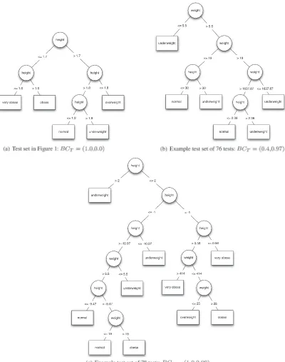
Some of these problems are illustrated with the bmiCategory example in Figure 1. The test set in the table achieves branch and path coverage but fails to highlight the bug in line 5; the inputs do not produce a body mass index (BMI) greater than 21 and smaller than 25 that would erroneously output ‘overweight’ instead of ‘normal’. Although mutation testing is capable in principle of highlight-ing this specific fault, this depends on the selection of mutation operators and their quasi-random placement within the code—there is no means by which to establish that a given set of mutations collectively characterizes what should be a truly adequate test set.
The fact that the given test set is unable to find this specific fault is merely illustrative. There is a broader point:source code coverage does not imply behavioural coverageand is not in itself a justifiable adequacy criterion. If a test set claims to fully cover the behaviour of a system, it ought to be possible to derive an accurate picture of system behaviour from the test inputs and outputs alone [2, 6, 7]. A manual inspection of only the inputs and outputs of the BMI example tells us virtually nothing about the BMI system; one could guess that increasing the height can lead to a change in output category. However, it is impossible to accurately infer the relationship between height, weight and category from these five examples. Despite being nominally adequate, they fail to sufficiently explore the behaviour of the system.
2.2. Behavioural test set adequacy
Behavioural adequacyis founded on the idea that, if a test set is to be deemed adequate, its tests
‘cover all aspects of the actual computation performed by the program’ [2]. In this context, the term
behaviourrefers to the relationship between the possible inputs and outputs of a program. In other
[image:3.595.117.486.521.686.2]words, it should be possible to infer a model from the program behaviour from the test set, which can accurately predict the outputs for inputs that have not necessarily been encountered. The concrete representation of this will vary depending on the nature of the program; a sequential control-driven
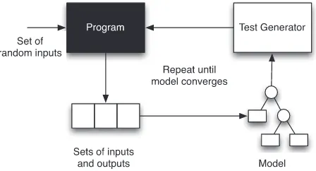
Figure 2. Basic ‘virtuous loop’ that combines testing with model inference.
system could be modelled as a finite-state machine; a data function might be represented by a differential equation, or a decision tree.
The idea of adopting this perspective to assess test adequacy was first proposed by Weyuker [2], who developed a proof-of-concept system that inferred LISP programs to fit input/output data. Since then, the idea of combining model inference with software testing has been comprehensively explored in several theoretical and practical contexts [6–14]. Much of this work has focussed on the appealing, complementary relationship between program testing and machine learning. The former is concerned with finding suitable inputs and outputs to exercise a given model of some hidden sys-tem, and the latter infers models from observed inputs and outputs. Together, the two disciplines can be combined to form a ‘virtuous loop’ where (at least in principle) it would be possible to fully automate the complete exploration of software behaviour.
This loop is illustrated in Figure 2. Of course, there are variants; different types of models, feed-back mechanisms and other sources of inputs can be fed in. Ultimately, the basic process is one of generating test sets, inferring models from their executions and (usually) using the models to iden-tify new test cases. The point at which the process terminates is also variable. Some approaches will only terminate once a strict condition has been established (e.g. the model can be demonstrated to be exactly accurate [12]). Others will simply terminate if time runs out, or no further test cases can be found that contradict the model [14].
A key factor that has prevented the widespread use of behavioural adequacy has been its practical-ity. So far, approaches have sought to make an adequacydecision, rather than obtain a quantitative
measurement. Models are deemed either accurate or inaccurate, accordingly test sets must be either
adequate or inadequate. This is problematic because the tasks of inferring an exact model and test-ing a model against a system are practically infeasible. In practice, this means that the combined processes of inference and testing tend to require infeasibly large numbers of test cases to converge upon the final adequate test set. If on the other hand a cheaper inference process is adopted that allows for an inexact model (cf. previous work by Walkinshawet al.[14]), there has been no reli-able means by which to gauge the accuracy of the final model, and to assess the adequacy of the final test set.
2.3. The probably approximately correct (PAC) framework
Much of the notation used here to describe the key PAC concepts stems from Mitchell’s introduction to PAC [15].
The PAC setting assumes that there is someinstance spaceX. For a software system, this would be the infinite set of all (possible and impossible) combinations of inputs and outputs. Aconcept
classC is a set of concepts overX, or the set of all possible models that consume the inputs and
produce outputs inX. The nature of these models depends on the software system; for sequential input/output processors,C might refer to the set of all possible finite-state machines overX. For systems such as the BMI example,C might refer to the set of all possible decision trees [15].
A conceptc X corresponds to a specific target within C to be inferred (we want to find a
specific subset of relationships between inputs and outputs that characterize our software system). Given some elementx (a given combination of inputs and outputs),c.x/ D 0or 1, depending on whether it belongs to the target concept (conforms to the behaviour of the software system or not). The conventional assumption in PAC is that there exists some selection procedureEX.c;D/that randomly selects elements inX following some static distributionD(we do not need to know this distribution, but it must not change).
The basic learning scenario is that some learner is given a set of examples as selected by
EX.c; D/. After a while, it will produce a hypothesis model h. The error rate ofh subject to
distributionD(errorD.h/) can be established with respect to a further ‘evaluation’ sample from
EX.c;D/. This represents the probability that hwill misclassify one of the test samples, that is,
errorD.h/P rx2DŒc.x/¤h.x/.
In most practical circumstances, a learner that has to guess a model given only a finite set of sam-ples is susceptible to making a mistake. Furthermore, given that the samsam-ples are selected randomly, its performance might not always be consistent; certain input samples could happen to suffice for it to arrive at an accurate model, whereas others could miss out the crucial information required for it to do so. To account for this, the PAC framework enables us to explicitly specify a limit on the extent to which an inferred model is allowed to be erroneous to still be considered approximately accurate (), and the probability with which it will infer an approximate model (ı).
It is important to distinguish between the term ‘correct’ in this context of model inference and the context of software testing. A model is ‘correct’ in the PAC sense if, for every input, it will return the same output as the subject system from which it was inferred, regardless of whether these outputs conform to the output expected by the systems’ developer. This is clearly different from the notion of functional correctness as applied to software. In this case, an output is only correct if it conforms to the developer’s intentions, or some abstract specification.
2.4. k-folds cross validation
In the testing context considered in this paper, there are several practical barriers that undermine the validity of applying PAC. PAC presumes that there are two large samples, selected under identical circumstances. However, in a testing context, there may only be a small selection of test cases available, and partitioning this sample into a training and a test sample could produce two highly dissimilar sets of features. Secondly, the available sample of test cases is unlikely to have been randomly selected from some fixed distribution; they might have been handpicked to deliberately achieve branch coverage for example.
This problem is also well established in machine learning. A practical alternative that has become the de facto standard for evaluating inferred models in such a context is known as k-folds cross
validation(CV) [16]. The basic idea is to, for somek, randomly divide the original set of examples
intokmutually exclusive subsets. Overkiterations, a different subset of examples is selected as the ‘evaluation set’, whilst the rest are used to infer the model. The final accuracy value is taken to be the average accuracy score from all of the iterations. This has the benefit of producing an accuracy measure without requiring a second, external test set.
2.4.1. Choosingk. One key parameter with the use of CV is the choice ofk. There is no firm advice
amount of time available. For example, if the number of examples is low and k is too high, the partition used for evaluation could be too small, yielding a misleading score. If there are lots of examples andkis high, it could take too much time to iterate through all of the partitions.
A common choice forkwhen CV is used to evaluate machine learning techniques is 10 (the CV technique as a whole is often referred to as ‘10-folds cross validation’). Alternatively, if the number of examples is not too high, it is possible to use ‘leave-one-out cross validation’, wherek Dn1, and the evaluation set always consists of just one example. Ultimately, however, given the lack of concrete guidance, the choice ofkis left to the user, and their judgement of the extent to which the set of examples is representative of the system in question.
2.4.2. Choosing a scoring function. Another important parameter is the choice of evaluation metric.
In other words, given an inferred model and a sample of inputs and outputs that were not used for the inference, how can we use this sample to quantify the predictive accuracy of the model? To provide an answer, there are numerous approaches, the selection of which depends on several factors, including the type of the model and whether its output is numerical or categorical.
For models that produce a single numerical output, the challenge of comparing expected outputs to the outputs produced by a model is akin to the challenge of establishing a statistical corre-lation. Accordingly, standard correlation-coefficient computation techniques (Pearson, Kendall or Spearman rank) can be used.
For non-numerical outputs, assessing the accuracy of a model can be more challenging. Accuracy is often assessed by measures that build upon the notions of true and false positives and negatives. Popular measures include the F-measure (the harmonic mean of Precision and Recall [17]), the receiver operating characteristic (ROC) and Cohen’s kappa measure on inter-rater agreement [18].
3. ASSESSING BEHAVIOURAL ADEQUACY
In this section, we show how the various notions presented in the previous section can be used to compute inference-based measures of test adequacy. We firstly present a PAC-based measure [4] in Section 3.1. This is then followed up by thek-folds CV measure in Section 3.2, which addresses some of the limitations of PAC.
3.1. Using PAC to quantify behavioural adequacy
[image:6.595.162.432.542.692.2]The PAC framework presents an intuitive basis for reasoning about test adequacy. Several authors have attempted to use it in a purely theoretical setting to reason about ‘testability’, to reformulate syntax-based adequacy axioms [6, 7, 10] or to place bounds on the number of tests required to produce an adequate test set [19].
The basic approach (as presented in [4]) is shown in Figure 3 (the arcs are numbered to indicate the flow of events). The test generator produces tests according to some fixed distributionDthat are executed on the system under test (SUT)c. With respect to the conventional PAC framework, they combine to perform the function ofEX.c;D/. The process starts with the generation of a test setA by the test generator (this is what we are assessing for adequacy). This is executed on the SUT; the executions are recorded and supplied to the inference tool, which infers a hypothetical model that predicts outputs from inputs. Now, the test generator supplies a further test setB. The user may supply the acceptable error bounds and ı (without these the testing process can still operate, but without conditions for what constitutes an adequate test set). The observations of test setBare then compared against the expected observations from the model, and the results are used to computeerrorD.h/. If this is smaller than, the model inferred by test setAcan be deemed to be
approximately accurate(i.e. the test set can be deemed to beapproximately adequate).
Theıparameter is of use if we want to make broader statements about the effectiveness of the combination of learner and test generator. By running multiple experiments, we can count the pro-portion of times that the test set is approximately adequate for the given SUT. If, over a number of experiments, this proportion is greater than or equal to1ı, it becomes possible to state that, in general, the test generator produces test sets that areprobably approximately adequate(to para-phrase the term ‘probably approximately correct’, that would apply to the models inferred by the inference technique in a traditional PAC setting).
3.1.1. Limiting factors. The PAC framework was developed as a purely theoretical concept. With
respect to testing, this has facilitated several useful calculations, such as establishing a polynomial bound on the number of random tests required to ensure behavioural adequacy [19]. More funda-mentally, it enables us to establish whether, at least in theory, certain systems are even ‘testable’ (i.e. whether or not there is a polynomial limit for a given system at all).
However, applying this framework in a testing context gives rise to several fundamental limita-tions (as mentioned in Section 2.4). The assumption that tests are selected at random from a fixed distribution is unrealistic. Effectively, this assumption would imply that there exists some fixed set of test inputs, from which both the test set and evaluation set are blindly selected. In reality, test sets are generated differently. For example, in attempting to ensure syntax coverage, one might select random inputs at first but then select further inputs that are influenced by the performance of the initial ones. One might also include particular test cases that are sanity-checks, and others that tar-get aspects of behaviour that are known to be particularly vulnerable to faults. This is not random selection; the distribution is not fixed, and the tests are not selected independently.
If we simply ignore these problems and use PAC regardless, there is a danger that the adequacy score is invalid. Ultimately, PAC is a statistical framework; it makes a probabilistic assumption that the final model is ‘approximately correct’. To be valid, statistical comparisons between groups rely on the presumption that the groups are sufficiently similar (to ensure that we are comparing ‘like with like’). This assumption can be easily violated in a testing context.
Aside from the manner in which samples are selected, there is also the (implicit) assumption that there are sufficient test cases from which to form a sufficiently robust comparison. Given that the comparison between the test set and the evaluation set is statistical in nature, statistical observations can only be confirmed with any confidence if they are derived from a sufficiently large number of observations. This runs counter to the general aim of keeping test sets as small as possible. Test sets that contain fewer than 10 test cases are very frequent but cannot be reasonably used in a PAC setting, because any statistical conclusion would lack sufficient statistical power.
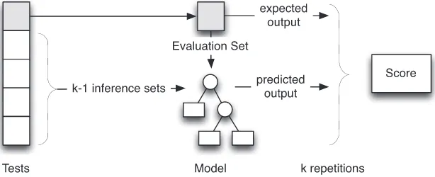
Figure 4. Illustration ofk-folds cross validation applied to behavioural adequacy.
3.2. Using CV to quantify behavioural adequacy
This section shows howk-folds cross validation (introduced in Section 2.4) can be used instead of PAC. This enables the use of a single large test set instead of two separate ones, which attenuates the problem of bias that can arise with PAC and reduces the number of tests required.
The process is illustrated in Figure 4. The scoring process starts with a single test set. The test set is partitioned intoksets of tests. Overkiterations,k1of the sets are used to infer a model, whilst the remaining set is used for evaluation. The result is taken to be the average of the scores.
CV is commonly used under the assumption that the given set of examples collectively reflect the complete range of behaviour of the underlying system. If this is the case, the resulting average score can be taken as indicative of the accuracy of the model inferred from the complete set. This assumption of a collectively representative set of examples does of course not always hold. In the case of program executions, a truly representative set is notoriously difficult to collect [1]. This gives rise to the question of what a CV score means when the test set is not necessarily complete or representative.
In this scenario, a CV score has to be interpreted in a more nuanced manner. Although CV scores are always ‘internally valid’ (they are always valid with respect to the data they are given), they are not necessarily ‘externally valid’; they can easily be misled by a poor sample. For example, looking forward to our inference of models from program executions, a set of examples that omits a prominent function in a program could yield models that all presume that no such function exists. Although the models may be very wrong, because they are all evaluated with respect to the same incomplete sample, they could still yield a very high CV score.
As a result, for scenarios where sets of examples fail to collectively expose the full range of behaviour of the system, there is the danger that the resulting score can be inaccurate. It is conse-quently necessary to interpret CV in a conservative light. If the score is high, it could well be due to a bias in the sample. A high CV score can at best corroborate the conclusion that an inference technique is accurate but cannot offer any form of guarantee. However, if the score is low, this is more reliably indicative of a problem, that is, with the sampling of the test set, or the inference of the model.
3.3. Combining code coverage with behavioural adequacy
As discussed in Section 2.1, source code coverage alone is insufficient when used alone as a basis for assessing test adequacy. Test sets that achieve code coverage often fail to expose crucial aspects of software behaviour. Capturing the set of executions that fully expose the relationship between the input to a program and its output generally entails more than simply executing every branch. It is this line of reasoning that underpins the PAC and CV-driven behavioural adequacy approaches.
the code is executed, but it is equally necessary to ensure that this code is executed sufficiently rigorously so as to ensure that all of its possible contributions to the program output are exposed.
This rationale underpins the argument that code coverage and behavioural adequacy are com-plementary [2]. Code coverage can guide the test selection towards executing the full range of behavioural features but cannot ensure that these features are executed in a sufficiently comprehen-sive manner. This aspect can however be assessed in terms of behavioural adequacy. The fact that the two measures are complementary suggests that they should both be taken into account when assessing the adequacy of a test set. This gives rise to our behavioural coverage metric, defined as follows:
Definition 1 (Behavioural coverage)
BCT D.C ovT; BAT/
For a given test setT,C ovT measures the code coverage (e.g. branch coverage) forT.BAmeasures the behavioural adequacy (either by PAC or CV) forT.
In order to impose an order on test sets in terms of their behavioural coverage, one could combine the two dimensions into a weighted average, similar to how the F-measure combines precision and recall. This is what we do in our optimisation (Section 4). Depending on the circumstances, however, it might be preferable to treat the two dimensions separately, for example, as part of a multi-objective optimisation.
This is not the first attempt to extend pure code coverage. However, past approaches to overcome the deficiencies of code coverage have lead to extended coverage metrics that consider code ele-ments only covered if they influence observable outputs (e.g. OCCOM [20] or OMC/DC [21]), or if they propagate to test assertions [22]. Behavioural coverage is different in that syntactic coverage and behavioural adequacy cannot easily be coerced into a single value, they are rather two dimen-sions: Code coverage representswhichparts of a program have been tested, and adequacy measures
how wellthey have been tested.
3.4. An example of behavioural coverage in action
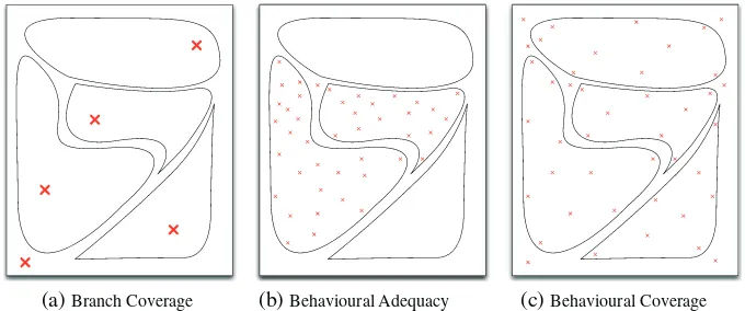
To provide an intuitive illustration of the rationale behind behavioural coverage, we consider the three diagrams shown in Figure 5. The area of each diagram is taken to represent the full range of input/output behaviour. Each zone within a diagram represents a distinctive feature of program behaviour.
Branch coverage of a program (Figure 5(a)) can often be achieved from a relatively small test set. In the BMI example, this ought to execute each behaviour of the program at least once. As one could easily conceive of a program involving conditional loops or complex data dependencies,
[image:9.595.129.469.551.693.2](a) Branch Coverage (b) Behavioural Adequacy (c) Behavioural Coverage
Figure 6. Decision trees inferred from different example test sets for the body mass index program.
it is therefore worth emphasizing that one could choose more rigorous code coverage criteria for behavioural coverage, such as Def-Use coverage [23] or MCDC [24]. However, merely executing a behaviour once is not necessarily sufficient by itself; as discussed in Section 2.1, a single execution of a feature is unlikely to expose any faulty behaviour.
tree is clearly incomplete; for example, none of the inferred decisions even depend on input ‘weight’. This incompleteness is reflected with a behavioural adequacy measurement of 0.0.
However, as shown in Figure 5(b), behavioural adequacy alone can be misleading. If a feature is not represented in a test set at all, this will not be reflected in the resulting assessment. Figure 6(b) shows a decision tree inferred from a set of 76 tests (selected from a random set of tests for illus-trative purposes) that cover only the cases of normal and underweight BMI values. Compared with Figure 6(a), the decisions are quite accurately reflecting the implementation with respect to the observed behaviour, which is reflected by a high adequacy score (0.97 using F-measure). However, the branch coverage value (40%) reveals that only two out of five cases are covered.
This leads us to the rationale for behavioural coverage, as shown in Figure 5(c). It seeks to com-bine the benefits of these two approaches. Accordingly, a test set should not only execute each individual feature but should do so sufficiently to achieve behavioural adequacy with respect to all of the features. An example of such a test set is used to infer the decision tree shown in Figure 6(c): All branches are covered, leading to 100% branch coverage. However, the adequacy score is now lower than that in Figure 6(b) (0.89), showing that although more behaviour has been covered, it has not been exercised with the same intensity as the subset of behaviour in Figure 6(b).
3.5. What about program correctness?
In this paper, we are exclusively concerned with the adequacy problem; assessing the extent to which a test set covers the observable program behaviour. The question of whether the tests are producing the correct results (theoracle problem) remains an open one. Note that this is not a problem specific to the notion of behavioural adequacy but applies to any adequacy measurement not based on a representation of intended behaviour (e.g. specification). For now, we have to presume that faults will manifest themselves in obvious ways (e.g. as program failures) or will be detected with the aid of assertions that have been produceda priori(either within the code or expressed as test properties). One further commonly suggested option is for the tester to manually inspect the test outputs. The problem here is that it can be a time-consuming, error-prone task. Potentially complex computations carried out by the SUT have to be replicated by the tester. Abstract functional requirements have to be reconciled with (possibly large numbers of) low-level inputs and outputs.
In this respect, inferring models from test executions can however provide assistance. Depending on the choice of inference algorithm, inferred models can provide an abstract, inspectable represen-tation of what has been tested. What might be thousands of test executions can often be summarized into a much more succinct abstract model.
4. GENERATING ADEQUATE TEST SETS
Having defined how to measure test set adequacy, we now turn to the question of how to produce test sets that are optimized in this respect. Whilst some traditional test generation problems such as branch coverage can be nicely framed in a way that makes it possible to use symbolic techniques to calculate test data, this does not immediately hold for behavioural adequacy. Furthermore, because a test set that achievesfullbehavioural adequacy could imply an unreasonably large number of tests, one might be content to trade off the adequacy for a smaller, more practical test set. Ultimately, this is an optimization problem calling for search-based testing techniques.
4.1. Search-based testing
To develop a search-based test generator for behavioural adequacy, it is necessary to define a suitable fitness function. According to Section 3, and in particular Definition 1, achieving this goal involves two distinct objectives: first, to execute allthe code of the method, and second, to
ade-quately do so. In other words, the fitness function should assess a test set in terms of its code
coverage, but also in terms of its ability to expose a sufficiently broad range of observable behaviour with respect to the executed code.
The tasks of fulfilling these two objectives are discussed in the following two subsections. This is followed by a more in-depth description of how the genetic algorithm applies the resulting fitness functions to home-in on suitable test sets.
4.2. Code coverage
The first objective is a traditional goal in test generation; a prerequisite to finding errors in a piece of code is that the code is actually executed in the first place. A reasonable approximation is articu-lated in the traditionalbranchcoverage metric: The proportion of possible true and false predicate outcomes that have been executed in a program (where 100% implies that all edges of the control flow graph are traversed). In principle, the approach could also be used in conjunction with more rigorous criteria such as Modified Condition/Decision Coverage (MCDC) [24], which may have a higher chance of revealing additional behaviour. Theoretical coverage criteria such as path coverage may help to expose more behaviour, but the path explosion problem caused by constructs such as by loops means that such criteria cannot generally be applied in practice. Furthermore, the link between behaviour and coverage remains tenuous: Executing loops with different numbers of iterations will not necessarily lead to relevant new behaviour.
We thus assume that a minimum requirement for any adequate test set is that all feasible (atomic) branches in the program have been executed. Achieving branch coverage is a classical objective in search-based testing, and the literature has treated this problem sufficiently. The fitness of a test set with respect to covering all branches is based on thebranch distancemetric, which estimates how close a logical predicate in the program was to evaluating to true or to false [25]. The branch distance for any given execution of a predicate can be calculated by applying a recursively defined set of rules (see [25] for details). For example, for predicatex 10andx having the value 5, the branch distance to the true branch ismax.0; 10x/D5.
A simple fitness function [26] is to sum up the individual branch distances, such that an optimal test suite would have a fitness value of 0. Some details need to be taken into account: First, branch distances need to be normalized to prevent any one branch from dominating the search. Second, we need to require that each branching predicate is executed at least twice, to avoid the search from oscillating between the true and false evaluation of the predicate (i.e. if the predicate is executed only once and evaluates to true, the search would optimize it towards evaluating to false instead, and once that is achieved, it would optimize it towards evaluating true again). Letdmi n.b; T /denote the minimum branch distance of branchbwhen executing test setT, and let.x/be a normalizing function in Œ0; 1(e.g. we use the normalization function [27]: .x/ D x=.x C1/), we defined
d.b; T /as follows:
d.b; T /D
8 ˆ ˆ ˆ < ˆ ˆ ˆ :
0 if the branch has been covered,
.dmi n.b; T // if the predicate has been
executed at least twice,
1 otherwise.
When generating adequate test sets, we require that the branch coverage for all branches in the set of target branchesBis maximized, that is, the branch distance is minimized. Thus, the overall branch fitness is defined as follows:
cov.T /D X bk2B
4.3. Behavioural adequacy
The second objective expresses how thoroughly this code has to be exercised with respect to its externally observable behaviour.
4.3.1. Using PAC and a validation set. To optimize behavioural adequacy using the PAC approach
(Section 3.1), we require two test sets. Consequently, our initial approach to compute behavioural adequacy [4] was to evolve pairs of test sets, where one will ultimately end up being the final test set, and the other one is the ‘evaluation’ set that is used to infer a model with WEKA [28], which is a widely used collection of machine learning algorithms. For a given pair of test sets.T1; T2/, the adequacyAcan be measured by inferring a model from T1, and comparing the predicted outputs from this model against the actual outputs from the program for the tests in setT2.
LetA.T1; T2; S /be a function that calculates the adequacy as described in Section 3.1 using a
scoring functionS (Section 2.4.2). Often, an adequacy value of 0 simply means that the number of samples is too small to draw any conclusions. Therefore, whenever adequacy is 0, we include the size of the test set in the fitness function, to spur the growth of test sets until adequacy can be reliably determined. We do this by including the size of test setT1 in the fitness function if adequacy is 0, such that larger test sets will be favoured by the search. To ensure that any adequacy value> 0has a higher fitness value, we normalize the size ofT1in the rangeŒ0; 1using the normalization function
[27] (see previous text), and otherwise add 1 if adequacy is> 0:
APAC.hT1; T2i/D
´
1CA.T1; T2; S / ifA.T1; T2; S / > 0,
.jT1j/ otherwise
A combined fitness function to guide test generation for adequacy can thus be defined as the weighted sum ofAPAC and the branch coverage values cov.T1/and cov.T2/(coverage of both test sets needs to be optimized):
fitness.hT1; T2i/D˛APAC.T1; T2/Cˇcov.T1/Cˇcov.T2/
The values˛andˇare used to weigh coverage against adequacy. For example, in our experiments, we usedˇ D1000and˛ D 1, which would cause the search to prefer even small improvements in coverage to large increases in behavioural adequacy. The reasoning for this choice of weight-ing is that a higher adequacy value may be misleadweight-ing if it is measured on an incomplete sample of behaviour. The search will thus initially be dominated by code coverage, and once the search converges on code coverage, exploration will focus more on behaviour. However, covering the exist-ing behaviour to a higher level of adequacy might in turn lead to coverage of additional syntactic elements, which the search would embrace and then explore to higher adequacy. Note that this weighting is an implementation choice we made for our experiments; in principle, it would also be possible to use multi-objective optimization to generate the test suites [29]. In this case, the result of the optimisation would be a Pareto-front of test sets, and the user would be able to choose between test sets with higher coverage and lower adequacy, or test sets with lower coverage but higher adequacy of the covered code.
As discussed in Section 3.1, there is a threat of sampling bias asT1andT2are not drawn indepen-dently from each other. The consequences of this are twofold. Firstly, this interdependence means that the final test sets are not as effective as they could be. Secondly, it can undermine the reliabil-ity of the final ‘behavioural adequacy’ score. A test set that is accompanied by an artificially high adequacy score that cannot be trusted by the developer undermines its value.
4.3.2. Usingk-folds cross validation. To overcome this drawback of the initial approach, we
Let A.T; S; k/ be the adequacy calculated as described in Section 3.2, where S is a scoring function (Section 2.4.2) andkis chosen as described in Section 2.4.1. Again, an adequacy value of 0 may indicate a too small sample size, such that the fitness function favours growth in that case:
AC V.T /D
´
1CA.T; S; k/ ifA.T; S; k/ > 0,
.jTj/ otherwise
Expressed as a weighted combination with the branch coverage value cov.T /, the fitness function to guide test generation for adequacy is thus defined as follows:
fitness.T /D˛AC V.T /Cˇcov.T /
4.4. Evolving adequate test sets with a genetic algorithm
The optimization goal is to produce an adequate test set. A test setT is a set of test casesti, and a test case is a value assignment for the input parameters of the target function. The number of tests in an adequate test set is usually not known beforehand, so we assume that the size is variable and needs to be searched for but has an upper boundBT. The neighbourhood of test sets is potentially very large, such that we aim for global search algorithms such as agenetic algorithm(GA), where individuals of the search population are referred to aschromosomes.
We generate the initial population of test sets randomly, where a random test set is generated by selecting a random numbern D ŒTmi n; Tmax, and then generatingntest cases randomly. A test case is generated randomly by assigning random values to the parameters of the method under test. Note that this is not a requirement; the initial population could also be based on an existing test set (e.g. [30]), for which one may intend to improve behavioural adequacy.
Out of this population, the GA selects individuals for reproduction, where individuals with better fitness values have a higher probability of being selected. To avoid undesired growth of the popu-lation (bloat [31]), individuals with identical fitness are ranked by size, such that smaller test sets are more likely to be selected. Crossover and mutation are applied with given probabilities, where crossover exchanges individual tests between two parent test sets, and mutation changes existing tests or adds new tests to a test set. These search operators have been explored in detail in the literature, and we refer to [32] for further details.
When using theAPACfitness function, the use of a validation set requires some adjustment: Here, a chromosome is a pair of test setshT1; T2i, in contrast to the single test setT used for the approach based on AC V. In general, it is not desirable that genetic material is exchanged between the first (test set) and the second (validation set). Therefore, in this case, crossover and mutation are applied to both test sets individually.
If the search is terminated before a minimum has been found, post-processing can be applied to reduce the test set size further. Traditional test set minimization uses heuristics that select subsets based on coverage information; in the case of adequacy, it is not easy to determine how an individual test contributes to the overall behavioural exploration. Therefore, in our experiments, we minimized test sets using a simple, but potentially inefficient, approach where we attempt to delete each test in a set and check whether this has an impact on the fitness.
5. EVALUATION
To evaluate the effects and implications of behavioural coverage, we have implemented a prototype providing the functionality of the BESTESTPAC and BESTESTC V approaches. The prototype takes as input a Java class and attempts to produce a behaviourally adequate test set for each of its methods (according to either of the PAC ork-folds CV heuristics). Currently, systems are limited to param-eters of primitive input and return values, although this will be extended to general data structures and stateful types in future work.
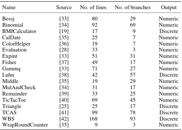
Table I. Study subjects.
Name Source No. of lines No. of branches Output
Bessj [33] 80 29 Numeric
Binomial [34] 92 69 Numeric
BMICalculator [19] 17 9 Discrete
CalDate [35] 25 7 Numeric
ColorHelper [36] 19 7 Numeric
Evaluation [28] 33 3 Numeric
Expint [33] 51 31 Numeric
Fisher [37] 49 17 Numeric
Gammq [33] 71 27 Numeric
Luhn [38] 42 57 Discrete
Middle [35] 19 29 Numeric
MulAndCheck [34] 31 17 Numeric
Remainder [39] 33 25 Numeric
TicTacToe [40] 69 45 Numeric
Triangle [25] 25 17 Discrete
TCAS [41] 99 78 Discrete
WBS [42] 168 93 Discrete
WrapRoundCounter [35] 9 3 Numeric
influencing BESTESTC V, whereas the fourth research question compares both approaches against a broad range of typical testing criteria (thus subsuming the original experiments in [4]). The specific research questions are as follows:
RQ1: What are the effects of learners, the valuekand evaluation metrics on the final behavioural adequacy score?
RQ2: Which configuration leads to test sets with the highest fault-detection ability?
RQ3: What is the relationship between behavioural adequacy and fault-detection ability?
RQ4: How does behavioural adequacy compare with traditional syntactical adequacy criteria?
5.1. Experimental setup
5.1.1. Subject systems. The set of classes selected for our experiments is shown in Table I. These are
selected (indiscriminately) from existing testing literature (referenced where possible). Because the purpose is to focus on particular units of functionality, we identify the particular method within each system that accepts the input parameters and returns the output value. Although an arbitrary number of other methods may be involved in the computation, our current proof-of-concept system requires the specification of a single point for providing input and reading output. As will be discussed in Section 6, our ongoing work is transferring this technique to other systems (e.g. abstract data types) that have multiple methods for providing input and output.
Our use of off-the-shelf machine learning algorithms imposes another restriction. We only selected systems that return primitive inputs and outputs (numbers, strings and Booleans). As dis-cussed in Section 2.4.2, these have been grouped into two categories: those that return a numerical or a discrete value. This has a bearing on the model inference and scoring techniques that can be applied.
5.1.2. Experimental variables. The experimental variables that were identified, along with the
values that were assigned to them, are presented below.
The SUT (Table I).
The machine learning algorithm. To establish the effect of this, we identified a broad range of algorithms that have been well established in machine learning literature and have been shown to excel for a wide range of different types of system. The selected algorithms are as follows:
The M5 learner and the M5Rules variant (numeric systems) [28] The AdaBoost learner (discrete systems) [44]
Multilayer Perceptron (neural net) learners (both numeric and discrete systems) [28] Additive Regression (numeric systems) [28]
The parameters of the BESTESTC V approach mentioned in Section 3:
The valuek. This was chosen from one of the four most commonly used values: 2, 5, 10 or
n1(leave one out (LOOCV)).
The evaluation function (to measure how accurate the inferred model is). We selected from F-Measure, kappa and area under the ROC curve and the correlation coefficient (all as computed by WEKA [28]).
5.1.3. Data collection. The described approaches have been implemented using EVOSUITE[32] as
framework for evolutionary search and the WEKA model inference framework [28]. Each learner was executed with its default WEKA parameter settings.
The experiments were systematically executed, using every possible combination of variables on every subject. Because the EVOSUITEevolutionary algorithms and some of the WEKA inference algorithms include a degree of stochasticity, there is a danger that this can lead to particularly lucky or unlucky results. To avoid any skew from this effect, every experiment was repeated 30 times with different random seeds, and results are statistically analysed. EVOSUITEwas configured to run for
10 min per run for each class and configuration; all other parameters were set to default values [45]. After the 10-min run, resulting test sets were minimized using a simple heuristic. For each testtin the resulting test setT, the fitness value was calculated for the test set without the test (T0 DTn¹tº). If the fitness value ofT0is worse than that ofT, the test is retained inT; otherwise, it is removed fromT (and the adequacy calculation for the next testt0would then be based onT0, rather thanT). For each execution of a test set, its behavioural adequacy and mutation score were recorded. The data collection was particularly time-consuming. For RQ1–RQ3, BESTESTC V had to be executed and assessed for every possible combination ofk, evaluation function and learner. For RQ4, both BESTESTC V and BESTESTPAC had to be executed and compared against a host of baseline test generation techniques (carried out by configuring alternative fitness functions in EVOSUITE). Again, to avoid accidental bias, each experiment for the baseline approaches was repeated 30 times with different random seeds. For each subject, configuration and seed, EVOSUITEwas run for 10 min. This should lead to a fair comparison, as the overhead of inferring models for BESTESTPAC and BESTESTC V is included in these 10 min. The following baseline test adequacy measures were used to drive test generation:
A test set optimized for branch coverage, where test sets are built to cover every logic branch in every method.
A test set optimized for branch coverage but expanded with random tests to match the average size of the BESTESTC V test sets (to investigate the influence of test set size).
A random test set that was generated to match the average size of the BESTESTC V tests. A test set optimizing the weak mutation score [46], where test sets were generated to expose
mutants.
A test set optimizing dataflow coverage, where test sets are optimized to cover as many as possible inter-method, intra-method, and intra-class definition-use pairs in the target class [47]. A test set generated using the original BESTESTPAC approach [4] (denoted ‘PAC’ in the plots).
This was run with the full set of machine learning algorithms and evaluation metrics.
This culminated in a total of 286 202 experimental configurations, totalling286 20210minD
5:4years of computational time. These experiments were executed on the University of Sheffield Iceberg HPC cluster‡. The full dataset is available online§.
5.1.4. Analysis techniques. To measure the effect of different factors (e.g. the choice of learner), or combinations of effects (required for RQ1–RQ3), we carry out grouped statistical tests. Because Shapiro–Wilks tests indicate that the data is non-normal, we cannot use analyses of variance and related measures such as partial eta-squared to assess effect sizes. Instead, we resort to non-parametric measures that do not presume normality.
To measure the effect of different factors (e.g. the choice of learner) on the adequacy and mutation scores, we use Cliff’sı[48]. This was primarily chosen because it is (a) well established and (b) simpler to interpret than other comparable measures. For more details about non-parametric effect size measurements, we refer to Peng and Chen [49]. Given a pair of groupsAandB(e.g. the group of mutation scores for two different classes), Cliff’sıgives the probability that individual scores forAare greater than those forB. Theıscore lies in the intervalŒ1W1, where negative numbers indicate the probability that all of the scores forAare smaller thanB, and positive numbers indicate the probability that all of the scores forAare greater thanB. A score of 0 indicates that the two distributions are overlapping.
Cliff’sıis a pairwise test. To investigate the effect of a particular factor (e.g. learner), we carry out every possible pairwise test for that factor (we compare the mutation scores for every pair of learners). The systematic approach used to run the experiments (Section 4) means that other factors are evenly represented in these groups. Because we only care about the relative distance between factors (and not which one was greater), we take the mean absolute value for all deltas, which gives us an overall effect size for the factor as a whole.
5.2. Results
5.2.1. RQ1—What is the effect of learners,kand evaluation metrics on the final behavioural
ade-quacy score. The aim of this research question is to investigate how the various factors affect the
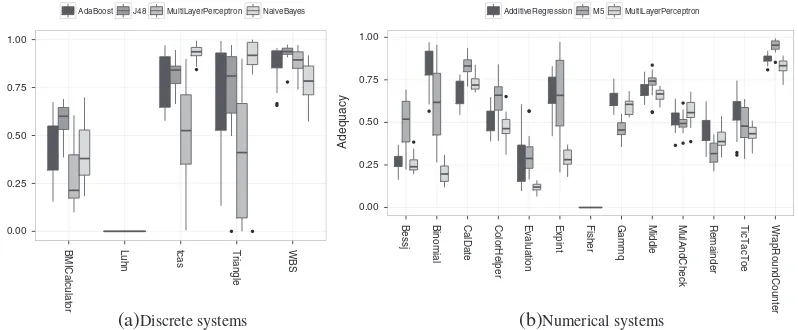
resulting adequacy score. Table II shows the Cliff’sı values, illustrating the extent to which dif-ferent factors contribute to the variance of the adequacy scores. To further provide an overview of the data, two box plots that summarize the interplay between the choice of learner and subject class are shown in Figure 7, and Figure 8 illustrates the effect of the evaluation metric for each of the discrete systems.
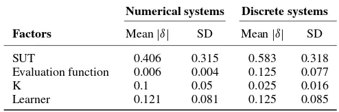
Learner: Taking the choice of class into account, the choice of asuitablelearner is important, with an averagejıjof 0.12 for both numerical and discrete systems. This is corroborated by the box plots in Figure 7; different learners can yield completely different adequacy scores. For example, under TCAS for discrete systems, the MultiLayerPerceptron neural net learner tends to produce low adequacy scores (mean of 0.51), whereas the NaiveBayes learner measures a mean score of 0.93.
In general, we observe that for discrete systems, the J48 (C4.5) and Naive Bayes learners con-sistently lead to higher adequacy scores than the AdaBoost and MultiLayerPerceptron learners. For numerical systems, depending on the system, either the AdditiveRegression or M5 algorithms lead to highest adequacy scores.
[image:17.595.175.422.617.699.2]System under test (class):The Cliff’sıvalues show that adequacy scores depend primarily on the system under test (the class). This is especially pronounced with the discrete systems, where the choice of class leads to an averagejıjof 0.58. This is to be expected; systems can vary substantially in terms of complexity, making it much harder to infer suitable models and derive useful test sets
Table II. Cliff’s delta with respect to adequacy scores.
Numerical systems Discrete systems
Factors Meanjıj SD Meanjıj SD
SUT 0.406 0.315 0.583 0.318
Evaluation function 0.006 0.004 0.125 0.077
K 0.1 0.05 0.025 0.016
Learner 0.121 0.081 0.125 0.085
0.00 0.25 0.50 0.75 1.00
BMICalculator Luhn tcas Triangle WBS
Adequacy
(a)Discrete systems
0.00 0.25 0.50 0.75 1.00
Bessj Binomial CalDate ColorHelper Evaluation Expint Fisher Gammq Middle MulAndCheck Remainder TicTacToe WrapRoundCounter
Adequacy
AdaBoost J48 MultiLayerPerceptron NaiveBayes AdditiveRegression M5 MultiLayerPerceptron
[image:18.595.100.499.71.236.2](b)Numerical systems
Figure 7. Adequacy scores by class and learner.
0.00 0.25 0.50 0.75 1.00
BMICalculator Luhn tcas Triangle WBS
Adequacy
Correlation FMeasure Kappa ROC
Figure 8. Adequacy scores for discrete systems by class and evaluation metric.
for some than others. This is also nicely demonstrated by the large variation between the individual classes as shown in Figure 7.
This gives rise to the question of which features of a system make it particularly easy or hard to infer an accurate model from the system. As we saw in the previous text, the learner does have an influence, but clearly less than the actual system under test. We conjecture that the main factor influencing this phenomenon is the testabilityof the system. In particular, Figure 7 shows two special cases: For the discrete systems,no configuration managed to achieve a positive ade-quacy score on the Luhn system. Similarly, for the numerical systems,no configuration managed to achieve a positive adequacy score for the Fisher class. We revisit Luhn and Fisher again in detail in Section 5.3.2.
[image:18.595.182.413.279.492.2]Value ofk: The choice ofk has a very slight impact for both numerical and discrete systems. The averagejıjis 0.01 for numerical systems, and 0.03 for discrete systems.
For numerical systems, higher values ofk tend to lead to higher values of adequacy. When all numerical configurations are ranked according to adequacy score, the top eight configurations have
kas LOOCV (the highest possible value). Of the bottom 10 configurations, six havek D2, whereas none of the top 25 configurations havekD2. The full table is provided in the accompanying dataset for this paper§.
Finally, there is a remark about the interpretation of these scores. The purpose of this research question is to investigate the relationship between the various factors (learner, k and evaluation metric) and the adequacy score. There is a temptation to conclude that those configurations that yield the highest scores are also the ‘best’ ones. This is however potentially misleading; a false high score could easily arise from the use of unsuitable configurations (Section 3.3). The next research question will therefore attempt to draw a link between adequacy and the actual performance: the ability to detect faults.
5.2.2. RQ2—Which configurations lead to test sets with highest fault-detection ability. To assess
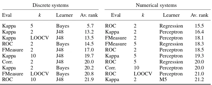
fault-detection ability, we resort to mutation analysis as a proxy measurement [50]. We calculated mutation scores using EVOSUITE’s built-in support for mutation analysis, which uses the same mutation operators as implemented in Javalanche [51] and the aforementioned study [50]. The muta-tion scores are averaged over 30 runs, to account for randomness in the evolumuta-tionary algorithm. The averagejıjresults, shown in Table III, assess the extent to which different factors affect the mutation scores. The top 10 configurations according to average rankings are displayed in Table IV.
[image:19.595.176.422.401.484.2]Before discussing the individual findings, it is important to discuss an intrinsic characteristic of the mutation data. As shown by the data in Table III, the choice of class has by far the largest effect on the eventual mutation score. In both numerical and discrete systems, the choice of system
Table III. Cliff’s delta with respect to mutation scores.
Numerical systems Discrete systems
Factors Meanjıj SD Meanjıj SD
SUT 0.849 0.277 0.86 0.291
Evaluation function 0.003 0.002 0.04 0.03
K 0.01 0.006 0.03 0.015
Learner 0.03 0.02 0.08 0.07
SD, standard deviation; SUT, system under test.
Table IV. Average rankings in terms of mutation score for different configurations of learner, kand evaluation function.
Discrete systems Numerical systems
Eval k Learner Av. rank Eval k Learner Av. rank
Kappa 5 Bayes 5.7 ROC 2 Regression 15.5
Kappa 2 J48 13.2 Kappa 2 Perceptron 16.4
Kappa LOOCV J48 13.5 FMeasure 2 Perceptron 18.1
ROC 2 Bayes 14.5 FMeasure 5 Regression 18.3
FMeasure 2 J48 17.0 ROC 2 Perceptron 18.5
Kappa 10 J48 19.7 Kappa 5 Perceptron 19.3
Corr. 2 J48 20.0 ROC 5 Regression 20.0
Kappa 2 Bayes 20.2 Corr. 10 Perceptron 20.0
FMeasure LOOCV Bayes 20.8 ROC LOOCV Perceptron 21.0
ROC 10 J48 21.9 Kappa 2 M5 21.2
[image:19.595.123.478.538.680.2]accounts for the biggest differences in score. This is explained by the fact that the average mutation scores were primarily stratified according to classes, where specific configuration options would only lead to relatively small deviations from the average mutation score for a given class. This is due to the fact that for a given class, the majority of mutants could be exposed trivially, byanytest. Only a small fraction of remaining mutants could serve to distinguish the truly rigorous test cases; a relatively small improvement in the mutation score could indicate a significant increase in the adequacy of the test set.
Despite the overwhelming variations in mutation score according to class, the results show that the other factors nonetheless have a significant impact of their own. The key findings are as follows:
For numerical systems, the choice of a suitable learner is the only factor to have a slight influence on the mutation score, with an averagejıjof 0.03.
For discrete systems, all other factors have a non-trivial effect on the mutation score. Eval and
khave averagejıjs of 0.03 and 0.04, respectively. The choice of learner has a comparatively much more significant effect, with an averagejıjof 0.08.
Looking at the specific configurations (the top 10 of which are shown in Table IV), the significant role of the learner is clear. The Naive Bayes and J48 (C4.5) learners consistently lead to the highest mutation scores for discrete systems (they dominate the highest-scoring 10 configurations but do not appear at all in the bottom 10). For numerical systems, it is a similar case for Additive Regression and MultiLayer Perceptron learners.
5.2.3. RQ3—What is the relationship between the adequacy score and the ability to detect defects.
Whilst investigating RQ1 and RQ2, it became apparent that the range of adequacy and mutation scores is sensitive to the configuration of BESTESTC V. An unsuitable configuration will overesti-mate adequacy scores. Accordingly, to answer this question, we assume that we are starting from a configuration that is capable of effectively exposing faults. So, given such a configuration, why is it effective? How and to what extent does adequacy contribute?
To establish this relationship, we therefore choose those configurations that led to the high-est mutation scores in RQ2, that is, those ranked highhigh-est for numerical and discrete systems in Table IV. Note that the earlier criticism on source code-based criteria holds also for mutation analysis (Section 2.1). That is, a high mutation score is merely a rough indicator of adequacy. Nevertheless, a sufficient exploration of a program’s behaviour should generally lead to high muta-tion scores. The chosen configuramuta-tions are thus those that performed best across all numerical and discrete systems (in some cases, certain configurations might achieve higher mutation scores on individual classes).
First of all, we want to establish whether there is a correlation between adequacy and mutation score; does an increase in adequacy imply a corresponding increase in mutation score? Calculating the Pearson correlation coefficient indicates a coefficient of0.18 for discrete systems and 0.02 for numerical systems. Clearly then, at face value, there is no positive correlation at all.
For a closer inspection, Figure 9 shows scatter plots relating the mean adequacy score to the mean mutation scores. It is important to bear in mind that each coordinate summarizes 30 actual recordings, which are often unevenly spread. Because there are too many points to plot in a useful way, the concentration of these points is indicated by the contour lines (the results of a 2D Kernel density estimation¶).
This points towards a more subtle relationship between the two factors that differ between the discrete and numerical systems. In the numerical systems, the mutation scores tend to be high, but there is a high variance in adequacy score (as indicated by the fact that the contours run across the plot in a relatively narrow band). However, for the discrete systems, both dimensions tend to be spread more evenly around particular coordinates for each system (as indicated by the more conical contours).
For Fisher, Evaluation (numerical) and BMICalculator (discrete), the results stand out; the muta-tion score is very high, despite a very low adequacy score. These programs are interesting because
0.7 0.8 0.9 1.0
0.00 0.25 0.50 0.75 1.00
Adequacy Score
Mutation Score
(a)Numerical systems: Eval=ROC, =2, learner = Additive Regression
0.75 0.80 0.85 0.90 0.95 1.00
0.00 0.25 0.50 0.75 1.00
Adequacy Score
Mutation Score
[image:21.595.172.427.90.618.2](b) Discrete systems: Eval=Kappa, =5, learner = Naive Bayes
Figure 9. Scatter plots relating adequacy scores to the normalized mutation scores for the two top configurations in Table IV.
for RQ1. Evaluation calculates a statistical correlation, where a test set has to contain pairs of num-ber sets as inputs that fulfil particular correlation properties. BMICalculator carries out a non-linear calculation from two numbers to compute a category; although its branches can be covered easily, this would not suffice to expose the underlying non-linear relationship between the input parameters and the output category.
If we restrict ourselves to programs for which the mutants cannot be trivially exposed (by leaving out Fisher, Evaluation and BMICalculator), effects on the correlation coefficients are observable. For discrete systems, the Pearson correlation rises from0.18 to 0.59, and for numerical systems, the correlation rises from 0 to 0.21. In summary, for programs where mutants are not trivially covered, a correlation emerges between adequacy and the mutation score. An increase in adequacy indicates an increase in the number of faults that are exposed by the test set.
Branch coverage remains the primary driver for mutation coverage. For numerical systems, the correlation between branch and mutation coverage is 0.59 (0.7 for the subset excluding Fisher, Evaluation and BMICalculator), and for discrete systems, it is 0.93.
Despite the fact that they are both positively correlated with mutation score, adequacy and branch coverage are not correlated with each other (Pearson correlations of0.02 for both numerical and discrete systems). This corroborates their complementary nature, as discussed in Section 3.3. The branch coverage objective increases the diversity of the test set to execute a larger proportion of program features. The extent to which these features are fully explored is in turn maximized by the adequacy score, which also tends to spur the exploration of additional branches that are particularly hard to reach. Ultimately, it is this synergy between the two that yields the higher mutation scores.
5.2.4. RQ4—How does BESTESTC V compare with existing adequacy criteria. To establish the
comparative performance of test sets generated using the BESTESTC V approach, we compared them against test sets generated to fulfil a selection of traditional, syntax-based criteria, as described in Section 5.1.3. All of the resulting test sets were compared in terms of their mutation score and size. The results for discrete systems are shown in Figure 10, and the results for numerical systems are shown in Figure 11.
To make such a comparison meaningful, it is necessary to pick a specific configuration for BESTESTC V . For this, it makes sense to select a configuration that is known to perform reasonably well (previous RQs have after all shown that there are several choices of model inference algorithm that perform very poorly). Accordingly, we selected the two configurations that had the highest cor-relations for discrete and numerical systems (as used in RQ3, those ranked highest for numerical
[image:22.595.97.498.480.681.2](a)Mutation Scores (b)Test Set Sizes
Figure 10. Comparison between BESTESTC V and alternative criteria for discrete systems. PAC, probably
(a)Mutation Scores
[image:23.595.100.503.77.393.2](b)Test Set Sizes
Figure 11. Comparison between BESTESTC V and alternative criteria for numerical systems. PAC, probably
approximately correct; CV, cross validation.
Table V. Cliff’s delta for comparison of mutation scores against BESTESTC V.
D. flow Branch PAC Mut. BranchC Rnd.
Numerical systems
Expint 1.000 1.000 0.034 1.000 0.952 1.000
Remainder 0.133 0.656 0.003 0.915 0.308 1.000
TicTacToe 0.949 0.882 0.037 1.000 0.510 1.000
Gammq 0.989 0.734 0.448 0.162 0.505 1.000
Fisher 0.900 0.833 0.100 0.000 0.002 0.167
Middle 1.000 0.570 0.175 0.944 0.486 1.000
Mul&Check 0.457 0.438 0.506 0.517 0.114 1.000 W.R.Counter 0.667 0.667 0.467 0.333 0.386 0.667
Col.Hlp 0.669 0.463 0.867 0.867 0.241 0.480
Bessj 0.728 0.460 0.092 0.374 0.442 0.539
Binomial 1.000 0.929 0.101 0.834 0.800 1.000
Eval. 0.984 0.986 0.500 0.033 0.500 0.967
CalDate 0.733 0.817 0.721 0.829 0.528 0.733
Discrete systems
Luhn 1.000 1.000 0.246 1.000 1.000 1.000
BMI 1.000 0.911 0.148 0.579 0.416 1.000
tcas 1.000 1.000 0.553 1.000 1.000 1.000
WBS 1.000 1.000 0.131 1.000 1.000 1.000
Triangle 1.000 1.000 0.082 1.000 0.070 1.000
[image:23.595.136.463.455.693.2]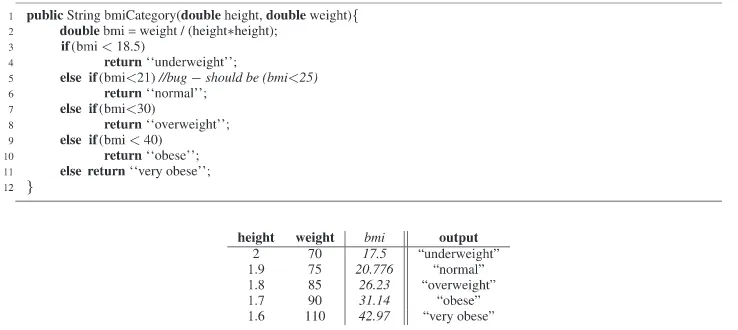
![Figure 3. Probably approximately correct (PAC)-driven test adequacy assessment [19]](https://thumb-us.123doks.com/thumbv2/123dok_us/7881545.184205/6.595.162.432.542.692/figure-probably-approximately-correct-pac-driven-adequacy-assessment.webp)