A double-loop learning approach to construct understanding of accumulation principles

(1)

A DOUBLE-LOOP LEARNING APPROACH

TO CONSTRUCT UNDERSTANDING

OF ACCUMULATION PRINCIPLES

A THESIS SUBMITTED FOR THE DEGREE OF

DOCTOR OF PHILOSOPHY OF

THE AUSTRALIAN NATIONAL UNIVERSITY

©

CHRISTOPHER ANTHONY BROWNE 2015

(2)

(3)

I declare that the work in this thesis is entirely my own and that to the best of my knowledge it does not contain any materials previously published or written by another person except where otherwise indicated.

(4)

(5)

For Lucy,

(6)

(7)

Acknowledgements

Climate Cafe, Lyneham PS, Turner PS

(teachers and students) for discussing Thesis Thesis Thesis Thesis Teaching Me Barry Newell (supervisor) for challenging Paul Compston (chair) for connecting Participants

(guinea pigs, students)

for trialling

Haley Jones (original supervisor)

for starting

System Dynamic Society, Anne LaVigne, Lees Stuntz Tracy Benson, Diana Fisher

(community) for nourishing Lucy (daughter) for inspiring Bridie (long-suffering) for tolerating supporting

Students (learners) for teaching RS Engineering (school) for employing Promoting Excellence & CHELT (Beth, Michael, Lyn & Kristie)

for recognising Richard Baker (mentor) for encouraging ANU community (university) for welcoming Jeremy Smith, Jamie Pittock & Shayne Flint

(course conveners) for allowing and enabling

Dash (dog) long walks

(8)

(9)

Abstract

In this thesis, I present a concrete learning activity to assist engineering and STEM students with no formal systems-thinking training develop improved mental models of accumulation principles. This thesis takes up Sterman’s 2008 challenge to create new methods to develop intuitive systems-thinking capabilities so that people can discover, for themselves, the dynamics of accumulation and impact of policies.

At the core of this research is a model for double-loop learning through construc-tionist inquiry. The scenario for the activity is the eﬀect of anthropogenic carbon emissions on the atmospheric carbon concentration. A hands-on activity was developed called Tubs & Pumps (T&P) as a physical analogue of the carbon cycle. However, the activity could be adapted to a range of dynamic problems.

Students manipulate the T&P system guided by a series of prompts, which encourage focused and informed group discussion about the given problem. A range of treatment conditions were used to investigate the eﬀect of prompts and assessment layout in the experiment. The results show that using targeted prompts can drastically improve the likelihood of students demonstrating a sound understanding of accumulation principles.

(10)

(11)

D.1 Summary of all workshop timings and courses...A21 D.2 Problems observed in the Trial workshop 1 responses...A24 D.3 Frequency and changes of responses in the Experimentation workshop...A26 D.4 Rubric for categorising graphical responses in the linear dynamics task...A38 D.5 Linear pretest and carbon cycle graph...A41 D.6 Summary of profile data across all workshops...A42 D.7 Linear dynamics results by graphical response...A42 List of boxes 2.1: Components of a typical bathtub test...23

4.1: A response demonstrating an algebraic solution...96

4.2: Survey response showing a positive response to knowing the outcome with an incorrect graph...103

4.3: Typical graphical responses for each of the five graphical response categories...105

4.4: Comparison of graphical responses categories with respect to Sterman & Booth Sweeney’s coding schema...106

4.5: Coding of graphical and written descriptions...109

4.6: Information presented on the scenario cards...114

6.1: Diﬀerent graphical responses with similar written description...150

(17)

Glossary

Key terminology

accumulation principles valid stock-and-flow behaviour

activity a set of protocols for interaction with the T&P system

carbon cycle the biogeochemical cycle describing the exchange of carbon

between stocks in the Earth system

CS cognitive science, field of knowledge

double-loop learning a model for learning based on the continuous refinement of

mental models based on observations in the real world

experiment a set of protocols to describe design of workshops used for data

collection

flow processes that change a stock

L&T learning & teaching, field of knowledge

mental model cause-and-eﬀect logic used in one’s decision-making

physical simulation a process of simulation using a physical system; in this instance, the T&P system

response the answers provided in the assessment sheet

SF failure stock-flow failure, a violation of accumulation principles

ST systems thinking, field of knowledge

STEM science, technology, engineering and mathematics

stock an entity that accumulates or depletes over time

stock-flow (SF) failure a perception of stock-and-flow relationships that violate conser-vation of mass principles

system dynamics a methodology for describing complex physical and social

systems

T&P tubs and pumps, the activity at the core of this thesis

T&P system a physical, manipulable model used for simulation

WG confusion written-graphical confusion, where the graphical and written

responses do not match

(18)

Terminology for workshop activities

Note: Additional terminology for the workshop methodology is in Part II.

Experiments

Checklist the early experiments based on checklist instructions

Simulation later experiment to test diﬀerent simulation activities

Dialogue later experiment to test focussed dialogue prompts

Experimental categories

PC physical simulation activity with checklist instructions

PW physical simulation activity with workbook instructions

MW mental simulation activity with workbook instructions

Assessment sheets

ER Emissions & Removals

AE Anthropogenic Emissions

AA Anthropogenic Additions

Treatment categories

Treatment categories are referred to using the acronym ‘experimental category–assess-ment sheet’, for example, PW-AA. Additional categories include:

PW-GD as PW with group diagram treatment condition

PW-SC as PW with scenario card treatment condition

PW-GDSC as PW-GD and PW-SC combined

Graphical-written categories

Summary groups that categorise results for both the graphical and written tasks

Sound AP sound accumulation principles (AP); graphs that show a decrease,

with a matching written description

WG confusion written-graphical (WG) confusion; where the graph does not match

the written description, such as a graph that increases with a description that calls for a decrease

SF failure stock-flow (SF) failure; where the graph has a matching description,

(19)

1 Introduction

Generation by generation universities serve to make students think: [to] learn progressively to identify problems for themselves and to resolve them by rational argument supported by evidence; [to] learn not to be dismayed by complexity but to be capable and daring in unravelling it.

- Boulton and Lucas (2008, p.9)

1.1 Context of the study

Engineers are first and foremost problem solvers. Each engineering specialisation has within it an abstract body of knowledge that makes sense of real-world observations. For example, civil engineers use force equations to optimise the design of infrastructure; electronics engineers simulate circuitry to debug, prototype and create the next generation of devices. There will always remain the need for these skilled problem solvers; however, society will need future engineers to work in truly interdisciplinary teams to solve problems that are increasingly complex, dynamical in nature, embedded in systems of systems, and unrecognised by today’s engineering educators.

The future engineer needs to be proficient with a broad range of problem-solving skills in order to approach these complex problems, in addition to the specialist knowledge currently taught in undergraduate engineering programs (King, 2008). The student engineer needs more than technical knowledge; they need room to develop into creative, capable and convincing problem solvers. Students must be able to construct their own knowledge and develop their intuition about problems based on rich experiences, beyond textbook-based instruction. To achieve this, engineering educators need to take up Boulton & Lucas’ (2008) challenge to create educational environments where students can be bold in unravelling complex problems. We need to create learning environments that help students understand how to think, so that they can be active learners in their future problem-solving activities.

(20)

world. Second-generation cognitive scientists have shown that human understanding of the world is based on experience, and is largely metaphorical. Modern metaphor theory (Lakoﬀ & Johnson, 2003) can provide strong guidance to those attempting to develop eﬀective teams of problem solvers by building on learners’ experiences with the real world.

Newell (2012) argues that the careful design of simple, manipulable activities is a basis for building powerful dynamical metaphors for the development of shared conceptual repertoires. For example, using Cuisenaire rods to understand mathematical operations, or interacting with low-order models to understand dynamic behaviour. These activities allow participants to communicate more eﬀectively and, hence, more likely to create informed and shared understanding on a topic. These hands-on physical experiences allow learners to eﬀectively think through a problem, visualise past and future behaviour, learn from the experience, and in turn develop their own mental models.

Creating a learning environment for both active learning and higher-order thinking is not straightforward, nor commonplace, especially in the context of the changing landscape of higher education in Australia. Technology is becoming more prevalent as a method of delivering content on an increasing scale, shown in the rapid expansion of Massive Open Online Courses (MOOCs) and other online teaching models. In the face of these trends, opportunities for eﬀective concrete, hands-on learning are increasingly important and increasingly rare.

(21)

People of good faith can debate the costs and benefits of policies to mitigate climate change, but policy should not be based on mental models that violate the most fundamental physical principles. The results suggest the scientific community should devote greater resources to developing public understanding of these principles to provide a sound basis for assessment of climate policy proposals.

- Sterman & Booth Sweeney (2007 p.236)

Further, education in science, engineering or mathematics does not appear to improve these test results (Sterman 2008). There is a need to re-think the prevailing passive and disconnected approach to STEM (science, technology, engineering and maths) education—from kindergarten through to graduate education—in the face of increasingly complex problems, such as climate change.

This thesis is a record of an attempt to improve undergraduate STEM students’ understanding of stocks and flows in the carbon cycle, although the principles and approach has application at all levels of education. Intuition is measured through the participant’s causal insight into the future behaviour of the carbon system. I do this through adopting a double-loop learning approach, where students can think, visualise, and improve their understanding through a physical simulation experience from which the learner can draw his or her own conclusions.

1.2 Problem statement

(22)

1.3 Aim and scope of the thesis

The aim of this thesis is to improve how engineering educators understand of the use of concrete experiences in the learning process. This work builds on the established insights of Argyris's single- and double-loop learning, where eﬀective learning is demonstrated through the development of mental models. In Figure 1.1a, a single-loop learning model is shown, whereby decisions are made based on feedback from the real world. However, it is only in Figure 1.1b that decision-making is improved through the development of mental models. In this thesis, the use of hands-on activities and prompts are investigated as a fundamental part of double-loop learning.

a) Real World

Information Feedback Decisions Mental Models of Real World Strategy, Structure,

Decision Rules

b) Real World

Information Feedback Decisions Mental Models of Real World Strategy, Structure,

Decision Rules

Figure 1.1: Learning loops describing how decisions are made based on observations of the real world from Sterman (2000). a) single-loop learning, where decisions are made without the development of mental models. b) double-loop learning, which requires the evolution of mental models based on experience with the real world. Variables at the head of an arrow are aﬀected by the variables at the tail of the arrows.

(23)

1.4 Research questions

The model in Figure 1.1 is developed into a double-loop learning model for physical simulation in Figure 3.12. The loops in Figure 1.1 are named, with the top loop describing physical simulation, the bottom right loop describing

scaﬀolded refinement, and the bottom left loop describing focussed dialogue.From this, three research questions arise, leading to three partially overlapping experiments:

Experiment 1: Scaﬀolded refinement

Does display of instructions and information have an eﬀect on decision-making?

Experiment 2: Physical simulation

Does representational form of simulation have an eﬀect on decision-making?

Experiment 3: Focussed dialogue

Do opportunities for focussed dialogue have an eﬀect on decision-making?

1.5 Significance and contribution

The research generates two outcomes of relevance in important areas of learning and teaching in engineering.

The first outcome is the T&P system itself. It is a tool for hands-on learning that systems educators can adopt and use to explore fundamental dynamical concepts. Although the computer has enabled students to simulate dynamical systems, basic concepts such as the ephemeral nature of flows can be easily misunderstood by the learner. This leads to conceptual modelling issues, such as SF failure through confusion between stocks and flows. The T&P activity is a hands-on simulation environment that can reduce this confusion, which makes it a worthy tool in the suite of learning activities for systems educators.

(24)

changed. These subtle changes made a significant difference to the way that students completed the exercise, with correct responses ranging from 11% to 76% depending on the prompts used. With the use of effective instructions, I have been able to complement the T&P activity with a pedagogical approach that uses prompts and social learning to improve the effectiveness of the activity.

The approach for scaﬀolding of new concepts for the learner through a concrete activity is relevant to engineering educators as they continue to challenge students to become problem-solvers today and into the future.

1.6 Structure of the thesis

This thesis consists of seven chapters, organised into three parts.

Part I. Background

Part II. Research Approach Part III. Synthesis

Part I. Background (Chapters 2 and 3). I introduce the study, and situate it

within the relevant literature. In Chapter 2, I outline a stock-and-flow represen-tation of the carbon cycle. Then I discuss the confusion observed in stock-and-flow thinking, in particular the SF failure around the anthropogenic disruption to the carbon cycle.

In Chapter 3, I discuss three overlapping perspectives for constructing knowledge: systems thinking, cognitive science and learning & teaching. These theoretical frameworks provide the background for the design of the T&P activity, and emphasise the importance of active learning environments and situating learning in the physical world. These concepts are of critical importance to student engineers, especially as they attempt to navigate complex and open-ended problems.

In Part II. Research Approach (Chapters 4 and 5), I describe the research

(25)

the T&P activity, the treatment conditions, assessment tasks, and the coding of responses. In Chapter 5, I present summary results, and detailed results for each experiment and for each task by treatment condition.

In Part III. Synthesis (Chapters 6 and 7), I take the lessons from the current

(26)

(27)

PART I BACKGROUND

Preface

Approaches for constructing shared knowledge of dynamical systems is the focus of Part I. The emphasis on shared knowledge is due to the fact that the problems future engineers will confront are likely to be more complex than an individual can solve alone.

Simulation models are a useful for engineers to expose their thinking about a problem before making changes to complex real-world systems. In this thesis, I investigate the use of a physical simulation activity to improve students’ thinking about the real-world carbon cycle, an important component of the dynamic Earth system.

Human activity is changing the Earth system to the extent that we have entered a new geological epoch: the Anthropocene (Crutzen, 2002). It is becoming widely recognised, and acknowledges a new geological period where human activities have a significant global impact on the Earth's ecosystems:

Human influence on the climate system is clear, and recent anthropogenic emissions of greenhouse gases are the highest in history. Recent climate changes have had widespread impacts on human and natural systems.

- Stocker et al (2013, p. 15)

(28)

In this thesis, I investigate whether the use of a physical simulation activity (the T&P activity) can provide a basis for adults to better understand the cause-and-eﬀect logic in the carbon cycle. The goal of the activity is to allow participants to correctly infer the required future trajectory of anthropogenic carbon emissions in order to stabilise the atmospheric carbon stock.

Part I is organised across two main themes:

Chapter 2: A discussion of the carbon cycle: the real-world context of the T&P activity. This includes a stock-and-flow representation of the carbon cy-cle (§2.1) and the previous work that recognised stock-flow (SF) failure (§2.2), specifically SF failure around the carbon cycle.

(29)

2 Stock-and-flow thinking and the carbon cycle

To suggest that we’re tackling climate change by building new mines and new power stations is simply absurd. I mean, it’s like someone who’s drunk at the end of the night at a party saying, “Look, I’ve switched to low-alcohol beer now. It’s OK”.

- Richard Denniss (ABC RN Breakfast, 2015)

A fundamental problem for system dynamics educators is helping students to distinguish between stocks and flows. Recently, many studies have highlighted stock-flow (SF) failure in students’ mental models of accumulation, in both linear and non-linear systems (Booth Sweeney & Sterman, 2000; Sterman & Booth Sweeney 2002; 2007; Cronin & Gonzalez, 2007; Cronin et al, 2009; Brockhaus et al, 2013; Sedlmeier et al, 2014; Kapmeier, 2004; Kapmeier et al, 2015). This confusion occurs when there is an inconsistency between the perceived behaviour of stocks (an entity that accumulates or depletes over time) when the flows (the rate at which that entity changes) are given in a described system.

Of particular concern is SF failure in relation to the anthropogenic additions to the atmospheric carbon concentration. At the 2007 National Climate Change Summit, then Opposition leader Kevin Rudd proclaimed “Climate change is the great moral challenge of our generation” (Kelly, 2007). However, studies have shown that public understanding of the dynamics of climate change is poor amongst even well-educated adults (Sterman & Booth Sweeney 2002; 2007).

In this chapter, I describe the dynamics of the carbon cycle in stocks and flows. I then describe the current arguments in the area of SF failure and testing of accumulation principles. Then I introduce the previous work investigating specifically SF failure in relation to the carbon cycle. This leads to Chapter 3, where I describe the background theory for T&P activity.

2.1 Dynamics of the carbon cycle

(30)

update of their work (Steﬀen et al, 2015) add the phosphorous cycle and changing land-use as higher-risk systems. These systems at higher-risk increase the uncertainty of the functioning and resilience of the Earth system.

The eﬀects of this change on the Earth system are many. In the Fifth Assessment Report of the Intergovernmental Panel on Climate Change (IPCC), the changes that are expected to occur towards the late 21st century are described as:

Virtually certain

- warmer and/or fewer cold days and nights over most land areas

- warmer and/or more frequent hot days and nights over most land areas

Very likely

- warm spells/heat waves. Frequency/duration increases over most land areas - heavy precipitation events. Increase in the frequency/intensity/amount - increased incidence and/or magnitude of extreme high sea level

Likely

- increases in intensity and/or duration of drought

- Stocker et al (2013)

There are a number of indicators that are used to measure the state of the climate system at various locations around the globe. These include land and ocean temperatures, precipitation rates, land-mass snow cover, extent of Arctic ice, ocean heat content, sea level change, the operation of the carbon cycle and other biogeochemical cycles. In this thesis, the carbon cycle is the only system of interest, specifically the anthropogenic disruption to the carbon cycle due to burning fossil fuels.

2.1.1 The carbon cycle in stocks and flows

(31)

amount of money in a bank account is controlled by the flow of deposits and withdrawals; the number of people in a department store at any one time is determined by the number of people entering and leaving the store.

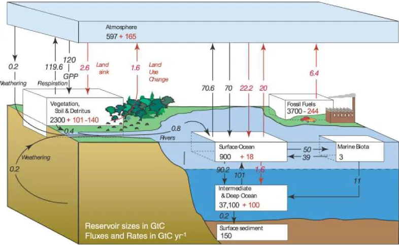
[image:31.595.117.510.270.511.2]

The major stocks and flows, as identified and quantified in the IPCC’s Fourth Assessment Report, are shown in Figure 2.1. The diagram shows the natural carbon stocks and flows and the anthropogenic perturbation of these stocks and flows. The quantities shown are as estimated in the mid-1990s.

Figure 2.1: Box diagram of Earth’s carbon cycle (Barker et al, 2007 Figure 7.3). Stocks (reservoirs) are shown as rectangular blocks; flows (fluxes) are indicated by arrows. Black numbers and arrows represent the natural cycle prior to anthropogenic influence. Red arrows and numbers indicate the anthropogenic perturbation.

(32)

The diagram shows a system that is largely in balance, with additions to and removals from each stock largely cancelling out. There are, however, small imbalances. Consider the flows directly connected to the atmospheric stock as seen in Figure 2.1. The natural cycle is in balance, with a circulation of approxi-mately 190.2 GtC/year. The anthropogenic disturbance upsets this balance, with a net amount of 3.2 GtC/year added to the atmosphere, mainly due to the 6.4 GtC/year added through the burning of fossil fuels.

Further, the rate of flows is changing, with the increased rate of burning fossil fuels. Feedback behaviour will also change the relationships in the carbon cycle; for example, as the global surface temperature increases, the temperature of the ocean increases, and its capacity to absorb carbon reduces.

In stock-and-flow notation, stocks are represented by rectangular boxes. An inflow is represented by an arrow pointing into a stock, and an outflow is represented by an arrow pointing out of a stock. The flows are represented by valves (taps), and clouds represent sources or sinks that are outside the system of interest. Variables are connected via influence links (arrows), which determine the nature of the relationships between the variables. Mathematical equations sit behind this graphical representation, and determine the relationships between the variables in a stock-and-flow diagram, allowing the model to be simulated over time.

(33)

Flux Atmosphere to Ocean

Net CarbonFlux to Deep Ocean

Flux Atmosphere to Biomass Flux Humus to

Atmosphere Flux Humus to Biomass Flux Ocean to Atmosphere Deep Ocean Temperature + + − Net Radiative Forcing − + + B B B +

Heat Stored in Deep Ocean

+

Insolation

Heat Stored in Atmosphere & Upper Ocean Carbon in Mixed Layer Carbon in Biomass Carbon in Humus Flux Biomass to Atmosphere Flux Biomass to Humus Carbon in Deep Ocean Carbon in Atmosphere Temperature Difference Fossil Carbon Fossil Fuel Consumption Atmosphere & Upper Ocean

[image:33.595.135.469.92.391.2]

Temperature Heat Exchange between Surface and Deep Ocean

Figure 2.2: Stock and flow diagram of the global carbon cycle and heat balance (Sterman, 2000 after Fiddaman, 1997). The stock of carbon in the atmosphere influences the heat stored in the atmosphere and upper ocean.

This stock-and-flow representation is a valuable tool for identifying how carbon moves through the carbon cycle. It clearly shows that the flows are two way, except the flow from the fossil carbon stock1_{. Even with only six stocks and nine} flows, it is diﬃcult to mentally simulate the behaviour of this model and determine what the likely future behaviour will be.

Despite the complex dynamics of the carbon cycle, the issue at the core is the net diﬀerence between the carbon additions to and removals from the atmosphere. Sterman oﬀers the bathtub metaphor (Kuznig, 2009) as a simpler model for thinking specifically about this relationship in the carbon cycle, shown in Figure 2.3. This ‘carbon bathtub’ model highlights the causal logic of the situation: if the additions exceed the removals, then the level of carbon in the atmosphere

(34)

[image:34.595.86.484.179.400.2]

increases; if the removals exceed the additions, then the level of carbon in the atmosphere decreases, and if the additions equal the removals, then the level of carbon in the atmosphere will remain steady in dynamic equilibrium.

Figure 2.3: Infographic describing the carbon bathtub (Holmes in Kuznig, 2009). The carbon bathtub highlights the important relationship in the carbon cycle: the net flow, which when positive will increase the level of the bathtub, when zero will stabilise the level, and when negative will allow the bathtub to drain.

If we take a bathtub approach to the model shown in Figure 2.1 and consider only those aspects of the carbon cycle that human activities can change directly, we are left with land-use change and the burning of fossil fuels. Rapid aﬀorestation could hypothetically—although not plausibly—balance out the burning of fossil fuels, and would require a significant reversal of current trends to replace the biomass removed through deforestation and other land-use change. Further, an increase in the vegetation carbon stock acts only as a buﬀer; living biomass that acts as a carbon sink also adds to the carbon in the atmosphere through respiration, and eventually decay, transferring carbon to both the soil and the atmosphere.

(35)

considered by some as a high-tech solution to restoring the carbon balance. The IPCC (2005) discuss the plausibility of geological and oceanic storage methods. Conceivably, if carbon could be captured at the point of emission, or even sucked out of the atmosphere, then balance could be restored. However:

All models indicate that CCS systems are unlikely to be deployed on a large scale in the absence of an explicit policy that substantially limits greenhouse gas emissions to the atmosphere.

- IPCC (2005 p.43)

Further, there are many gaps in knowledge about how CCS will aﬀect the Earth system, especially in the example of deep ocean carbon storage. With such uncertainty, it would be dangerous to consider this as a solution to reducing the stock of carbon in the atmosphere. Further, doing so could lead to reduced attention to strategies for mitigation.

Carbon-bathtub thinking then leaves only one viable option to stop the atmospheric carbon concentration from increasing: reduce the burning of fossil fuels immediately to zero. A key insight from this observation is that this action will only stop the stock of atmospheric carbon from increasing, and will not reduce it on the required time scale.

This is the educational challenge: participants in the T&P activity should be able to use the system as a physical analogue to think through this problem by experi-encing the interaction over time of stocks and flows. This should help them to realise that the atmospheric carbon stock will continue to rise unless the anthro-pogenic carbon emissions decrease to zero.

2.1.2 Anthropogenic carbon emissions over time

(36)

The trajectory of the carbon emissions from the burning of fossil fuels is shown in Figure 2.4, along with the resultant atmospheric carbon levels. The carbon emissions graph (Figure 2.4a) is a spline curve fitted to the atmospheric CO2 record. This record is based on ice core data before 1958. From 1958, it is based on the yearly averages of direct observations from the Mauna Loa and South Pole observatories. The atmospheric CO2 concentration graph (Figure 2.4b) is an estimate based on a compendium of energy use, with a consistent record from the United Nations since 1950.

a) 550 600 650 700 750 800 850 Year

1750 1770 1790 1810 1830 1850 1870 1890 1910 1930 1950 1970 1990 2010

0 2 4 6 8 10 Year

1750 1770 1790 1810 1830 1850 1870 1890 1910 1930 1950 1970 1990 2010 Global Carbon Emissions from Fossil-Fuel Burning, Cement Manufacture

and Gas Flaring 1751-2010

Atmospheric Carbon  

(using ice core data 1750-1957, and direct observation 1958-2010)

Carbon emissions per year

(GtC/year

)

Atmospheric Carbon (GtC

)

[image:36.595.86.446.252.584.2]

b)

Figure 2.4: Anthropogenic carbon emissions and atmospheric carbon levels (c1750-2010) a) global carbon emissions from fossil-fuel burning, cement manufacture and gas flaring (1751-2010), b) atmospheric carbon levels (1750-2010). Source: global carbon emissions (Keeling et al, 2005; Scripps, 2015); atmospheric CO2 concentration (Boden et al, 2013).

(37)

What will happen to the future atmospheric carbon concentration is of major concern to scientists and policy-makers alike. The argument about planetary boundaries put forward in Rockström et al (2009) is primarily that the goal should be to keep all Earth’s systems in balance. When any of the boundaries are exceeded, it puts at risk the other components of the system. Given the current circumstances, a 2°C temperature rise is considered to be both the upper limit of this safe operating space, but also a best-case scenario. In 2009, the Copenhagen Accord recognised the extent of the problem2_:

We underline that climate change is one of the greatest challenges of our time. We emphasise our strong political will to urgently combat climate change in accordance with the principle of common but diﬀerentiated responsibilities and respective capabilities. To achieve the ultimate objective of the Convention to stabilize greenhouse gas concentration in the atmosphere at a level that would prevent dangerous anthropogenic interference with the climate system, we shall, recognizing the scientific view that the increase in global temperature should be below 2 degrees Celsius, on the basis of equity and in the context of sustainable development, enhance our long-term cooperative action to combat climate change. We recognize the critical impacts of climate change and the potential impacts of response measures on countries particularly vulnerable to its adverse eﬀects and stress the need to establish a comprehensive adaptation programme including international support.

- UNFCCC (2009, p.1)

Despite this apparent political consensus, action has been lacklustre. Political arguments aside, a best-case benchmark for all negotiations is bringing anthro-pogenic emissions back to 1990 levels by (or after) 2020. In 1990, approximately 6.1 gigatons of carbon were released into the atmosphere (Keeling et al, 2005), which is still a significant annual addition to the atmosphere.

(38)

Cumulative emissions of CO2 largely determine global mean surface warming by the late 21st century and beyond. Most aspects of climate change will persist for many centuries

even if emissions of CO2 are stopped. This represents a

substantial multi-century climate change commitment created by past, present and future emissions of CO2.

- Stocker et al (2013 p.27)

The problem is, as described, the greatest moral challenge of our generation.

2.2 Stock-flow (SF) failure

In this section, I outline the recent work in the area of SF failure, before describing SF failure in relation to the carbon cycle.

Previous work around SF failure focusses on testing understanding of systems through either identifying features of the system, such as the point in time that a stock is at its minimum or maximum level, or by visually integrating the flows to show the behaviour over time of the stock. Studies examining SF failure to date have largely shown that participants have a poor intuitive understanding of the dynamics in stock-and-flow systems. Notable findings are that:

• highly educated adults have a poor understanding of simple stock-and-flow problems, and results often violate the law of conservation of mass (Booth Sweeney & Sterman, 2000; Sterman & Booth Sweeney, 2002; 2007; Cronin & Gonzalez, 2007), such as the belief that an increase in the rate of flows would lead to a stabilisation of the accumulation (see the correlation heuristic in Figure 2.5).

(39)

• varying cover stories of similar dynamic systems shows little improvement of understanding; for example, using everyday examples such as water in a bathtub, money in a bank account, or people in department store (Kapmeier, 2004, Cronin & Gonzalez, 2007; Cronin et al, 2009; Kapmeier et al, 2015)

In the previous work listed above, a small amount of priming is typically given, and participants use their experience of the real world to inform a decision during an assessment exercise. Typically, the exercise itself does not prompt the participant to question, orientate or improve their mental model of the problem prior to assessment.

There are, however, some promising observations in testing SF failure. Cronin et al (2009) note that outcome feedback helps students to achieve the correct answer, but that improvement is gradual. Formal system dynamics instruction improves understanding of stock-and-flow systems; however, a minority of students after graduate-level training in system dynamics still appear to be confused by stocks and flows (Sterman 2010).

A brief summary of this previous work is shown in Table 2.1. Here, test type describes the context of the study for reference. A common approach in these studies is to provide a range of assessment tasks which involve “calculus without mathematics” through graphical integration and diﬀerentiation (as described in Sterman, 2000 §7.1). Success rates, typically defined as the proportion of students providing a correct response, show the range (low to high) of correct results for treatment conditions in the given task.

(40)

[image:40.595.85.482.115.589.2]

Table 2.1: Overview of key previous SF failure studies, including test type, assessment task, treatment conditions and range of indicative correct response rates

Test type Assessment task and treatment conditions

correct reported % low % high Booth Sweeney & Sterman (2000)

bathtub test graphical integration 46% 83%

cashflow test graphical integration 51% 77%

manufacturing case graphical diﬀerentiation 32% 50%

Sterman & Booth Sweeney (2002)

zero-emissions task graphical integration and written (CO2) 22% 36%

graphical integration and written (temperature) 20% 46%

stable concentration task multiple choice and written 18% 69%

Sterman & Booth Sweeney (2007)

340ppm task multiple choice, graphs: emissions with/without

removal

‘falling’: 66%-89%

400ppm task multiple choice, graphs: emissions with/without

removal

‘falling’: 30%-49% Cronin & Gonzalez (2007)

department store task identification; store and bank context (accumulation) 29% 43%

distractor point identification; line and triangle (accumulation) 23% 42%

Cronin et al (2009)

department store task identification; multiple representation (accumulation) 31% 69%

identification; multiple contexts (accumulation) 17% 38%

identification; feedback and no feedback 12% 21%

identification; priming with system dynamics 53% 68%

Sterman (2010)

department store task before and after system dynamics training improved: 24.7% to 46.1%

Brockhaus et al (2013)

square wave succession of stocks, tubs and bath context 44% 67%

triangle succession of stocks, tubs and bath context 41% 61%

discontinuous task succession of stocks, tubs and bath context 22% 44%

Sedlmeier et al (2014)

square wave succession of stocks, animations ~32% 60%

(41)

Box 2.1: Components of a typical bathtub test (summarised and reproduced from Sedlmeier et al, 2014). The written description supplements the graphical representation of the problem, providing numerical information to help students compute the level of the stock over time.

Written description

The flow diagram indicates a constant outflow of 50 litres per minute but a variable inflow of 75 litres per minute for the first four minutes that diminishes to 25 litres per minute for the next four minutes and repeats this pattern once. The bathtub has 100 litres of water at time t=0.

Graphical description

The inflow and outflow rates A ‘correct’ solution

showing the corresponding stock level

Although the task shown in Box 2.1 is a relatively simple visual integration task, cohorts of students have failed to perform well. A number of strategies for reducing this type of SF failure have been proposed, such as providing adequate preparation, or instruction designed specifically to reduce the confusion between stocks and flows. However, at this stage no intervention has been able to provide a clear direction for improving participant’s understanding of accumulation, including formal education.

Given these results, the even shorter exposure to stock-and-flow concepts provided in short academic and commercial

training workshops is highly unlikely to be eﬀective in

(42)

they have far more training in STEM and other quantitative disciplines (economics, business) than the average person. Still their understanding of stocks and flows prior to exposure to the course is extremely poor. Further research into the failure of the educational system to provide such basic concepts, and eﬀective methods to teach these concepts in the K-12 grades, is sorely needed.

- Sterman (2010, p. 331)

There is a passionate movement for teaching systems thinking from an early age in the American education system (K-12). Forrester (2009) tells us that “any child who can fill a water glass or take toys from a playmate knows” about accumulation. Draper’s experience of teaching high-school physics, including topics such as thermodynamics, using stocks leads him to think:

Systems thinking, like any thinking paradigm, should be invisible—a natural way that people think about the world. In Barry Richmond’s words, it should be “the water we swim in.” Just as most of us don’t really deliberately choose to use inductive reasoning for a specific problem and deductive reasoning for a diﬀerent problem (we just figure stuﬀ out), people do not have to consciously know that they are using systems thinking for any particular problem. Instead, we should always be thinking in terms of feedback and circular causality. This principle also has to be applied to the teaching and to the learning of systems thinking and system dynamics. People do not have to know they are learning about the science of systems thinking or system dynamics. They just need to be taught, from the beginning, that the world around is in made of dynamic, interconnected systems and that there are tools we can use to understand these dynamic relationships.

- Draper (2010, p. 53)

(43)

amongst preschool children. For example, a storyline that oscillates between good and bad is a ‘crown’ story. Students transfer this metaphor to their everyday experience: “I’m having a ‘crown’ day.”

Previous work from the system dynamics community has shown that the carbon cycle is a topic where innovative teaching methods are needed to address SF failure.

2.2.1 SF failure and the carbon cycle

Developing an intuitive understanding about the dynamics of accumulation of carbon in the atmosphere is the specific problem that the T&P activity examines. Sterman & Booth Sweeney’s work (2002; 2007) shows that there is confusion between the rate of flows of carbon into the atmosphere and the corresponding changes in the level of the stock of carbon in the atmosphere. This confusion can contribute to poor policy decisions, such as the belief that a reduction of the rate of carbon emissions will also lead to a correlated reduction of the atmospheric carbon concentration.

Sterman & Booth Sweeney’s work considered many scenarios around the dynamics of the climate system, including the accumulation of CO2 in the atmosphere and the global temperature changes resulting from increased radiative forcing. The CO2 tasks involved questioning participants about the required action to stabilise the atmospheric carbon concentration at diﬀerent levels with and without consideration of removal of carbon from the atmosphere.

(44)

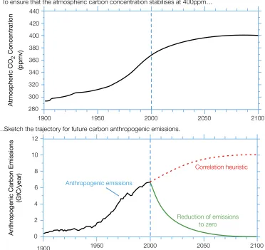
The correct answer to achieve the stabilisation of atmospheric CO2concentration is to reduce the anthropogenic emissions to zero, as shown in the bottom graph in Figure 2.5. The correlation heuristic shown would result in a rapid growth of the atmospheric CO2concentration. In the Sterman & Booth Sweeney study, 48% of participants in this task drew a graphical response of future emissions falling from current rates.

440

420

400

380

360

340

320

300

280

1900 1950 2000 2050 2100

Atmospheric CO

2

Concentration

(ppmv)

12

10

8

6

4

2

0

1900 1950 2000 2050 2100

Anthropogenic emissions

Anthr

opogenic Carbon Emissions

(GtC/year)

…Sketch the trajectory for future carbon anthropogenic emissions.

To ensure that the atmospheric carbon concentration stabilises at 400ppm…

Reduction of emissions to zero

[image:44.595.90.462.213.564.2]

Correlation heuristic

(45)

Further, Sterman & Booth Sweeney observed the correlation heuristic in the 340ppm task, where the atmospheric CO2 concentration falls rapidly from 2000 levels to 340ppm. 79% of participants drew a trajectory that had carbon emissions falling in a similar shape. However, to achieve a reduction in the atmospheric CO2 concentration, the carbon emissions would have to fall below zero. This example demonstrates the prevalence of SF failure in the area. Results for their ER condition, where a removals trajectory was also considered, showed further confusion, leading to their concern about SF failure in relation to the carbon cycle.

(46)

(47)

3 Constructing shared knowledge

The perceived threat from exposing our thinking starts early in life and, for most of us, is steadily reinforced in school—remember the trauma of being called on and not having the “right answer”—and later in work.

- Peter Senge (2006)

As Sterman & Booth-Sweeney (2002; 2007) note, adopting a wait-and-see approach about climate change is likely when the dynamics of the carbon cycle are not well understood. In this chapter, I provide the background rationale for using the T&P activity to address Sterman’s (2010) call for eﬀective methods to teach stock-and-flow concepts.

There are three overlapping perspectives through which the background is presented. The first is the systems thinking (ST) perspective, specifically with improving the ST capabilities of the educated public. Second, approaches in

cognitive science (CS) explain how our understanding of the world is influenced by conceptual metaphors and how knowledge is framed through our embodied mind. And third, approaches in learning and teaching (L&T) provide inspiration for a new way of framing ST learning. ST is, at its simplest, an approach for interpreting the world, just as the theoretical foundations of the design sciences, physical sciences and the social sciences are.

Although theoretical underpinnings of the three diﬀer significantly, there is an intersection of ideas when it comes to understanding how knowledge is constructed through experience with the real world.

Take, for example, these observations from the diﬀerent fields:

Systems Thinking observations

Any child who can fill a water glass or take toys from a playmate knows what accumulation means. (Forrester, 2009)

(48)

Cognitive Science observations

Our experiences with physical objects (especially our own bodies) provide the basis for an extraordinarily wide variety of ontological metaphors, that is, ways of viewing events, activities, emotions, ideas, etc., as entities and substances. (Lakoﬀ & Johnson, 2003)

Learning & Teaching observations

The learner constructs knowledge inside their head based on experience. Knowledge does not result from receipt of information transmitted by someone else without the learner undergoing an internal process of sense making. (Martinez & Stager 2013)

Children learn to speak, learn the intuitive geometry needed to get around in space, and learn enough of logic and rhetorics to get around parents—all this without being “taught.” (Papert 1980)

The intersection of these ideas is the focus for my review into background theory for the T&P activity.

Mental models

The starting point for this investigation is how the systems thinking community approaches thinking about thinking, particularly through the ST community’s description of mental models. There are three attributes common to definitions of mental models (Meadows, 2008, pp. 86-87; Sterman, 2000, pp. 15-29; Richmond, 2010; Senge, 2006; Maani & Cavana 2007). These attributes are that mental models:

• represent a subset of the real world (bounded rationality)

• are built from experience with the real world (an experiential abstraction)

• are incomplete and therefore diﬃcult to simulate (dynamically deficient)

(49)

decisions are made reactively to the information feedback observed in the real world. In this model, the learner doesn’t change their thinking about the problem, and continues to make the same mistakes without learning.

Real World

Information Feedback Decisions

[image:49.595.248.386.156.259.2]

Bounded Rationality

Figure 3.1: Influence diagram of bounded rationality as the first attribute of mental models, where information is derived from the real world, and decisions are made based on information from the real world observation.

I use the second attribute—experiential abstraction—to describe the refinement of mental models based on experience with the real world. In this feedback loop, information from real-world decisions are used to improve mental models. With the inclusion of the third attribute—dynamical deficiency—comes the capacity to change strategy and decision rules. In a learning context, this can be described as process learning, rather than learning as the skill of reciting content and facts. The student learns how to learn, and is readily able to adjust their decision-making process based on changes to their mental models. The addition of these two loops are shown in Figure 3.2.

Real World

Information Feedback Decisions

Mental Models of Real World

Bounded Rationality

Dynamical Connections

Strategy, Structure, Decision Rules

Experiential Abstraction

[image:49.595.207.426.504.707.2]

(50)

In this chapter, I examine the positive approaches that each perspective brings to facilitating development of these attributes of mental models, and in turn double-loop learning. The core ideas presented in this chapter are shown in Figure 3.3, and will be explored in the sequence: systems thinking, cognitive science, then learning & teaching.

Real World Information Feedback Decisions Mental Models of Real World

Bounded Rationality Dynamical Connections Strategy, Structure, Decision Rules Experiential Abstraction

2. Facilitating Experiential Abstraction

ST Model creation tools

CS Framing

L&T Scaffolding

1. Recognising Bounded Rationality

ST System archetypes

CS Conceptual metaphors

L&T Transitional objects 3. Creating Dynamical Connections

ST Group model building

CS Shared conceptual repertoires L&THigher-order thinking skills

KEY

ST systems thinking

CS cognitive science

L&Tlearning & teaching

Figure 3.3: Annotated influence diagram of background theory for aspects of the double-loop learning model, as seen from the ST, CS and L&T perspectives. This diagram represents the structure of this chapter.

Throughout this chapter, I refer to the carbon cycle to demonstrate concepts. Understanding the anthropogenic impact on the carbon cycle requires a clear, shared understanding of the problem in order to make informed decisions about possible pathways for the future of our planet. I also refer to the development of the T&P activity, described in Chapter 4, the goal of which is for participants to construct their own intuitive understanding (reliable mental models) of the relationship between anthropogenic carbon emissions and atmospheric carbon levels.

3.1 A Systems Thinking perspective on constructing knowledge

(51)

constructing mental models, then simulating the models to draw conclusions. Mental models provide a framework for thinking, understanding and learning, and hence their study is central to building eﬀective learning environments.

ST texts commonly introduce mental models as a background for describing how cause-and-eﬀect logic is built. Mental models are commonly used in this context to explain why systems behave unexpectedly. When a formal model that has been carefully created behaves in a way that is not expected during simulation, it is likely due to the modeller’s incomplete mental model that guided the construction of the formal model. When our mental models are challenged, there is an opportunity for learning by understanding how they could be improved.

An example is a student seeking to perform well in an exam. His or her previous experience with exams may lead to forming a mental model that cramming before an exam is an eﬃcient way to perform well. This strategy may work for some time and on some topics, but when exams become more diﬃcult, the strategy will no longer work. The reflective student will revisit their mental model about exams in order to improve their performance by, for example, adopting better study habits.

I will discuss how the systems thinking community develops the three attributes of mental models. First, I will discuss tools that the ST practitioners use to make bounded rationality explicit, such as model boundary charts, dynamic hypotheses and behaviour over time graphs. Then, I will discuss group model building as a tool for creating dynamical connections. To complete the ST perspective, I will discuss system archetypes and other small-order feedback structures as a tool for facilitating experiential abstraction.

3.1.1 Systems Thinking methods to recognise bounded rationality

(52)

models are further flawed because they exist in our minds. They are perpetually in draft form, as the causal chains are challenged and revised continuously to match the world we experience.

Mental models exist in one’s mind, and are not usually formally described. Although they may have been built from vast experience of the system of interest, it is difficult for a single person to understand the world from multiple perspectives. Because of this, an individual’s mental models are often an incomplete representation of a given problem – they exhibit bounded rationality. The ancient Sufi story of the blind men and the elephant is commonly used to explain this (Meadows, 2008). In this story, many men each hold a different part of the elephant and each have a completely different understanding of both what it is and what its purpose might be. This story provides an example of why sharing, and then challenging, mental models of a problem can result in a deeper understanding of the system of interest.

The bathtub metaphor is a fundamental framework for systems thinking and the T&P activity. A visualisation of the bathtub metaphor is shown in Figure 3.4, showing the main components and relationships. This visualisation shows only some of the factors that could be included in a bathtub system; it is a simplifi-cation that represents a subset of the real world.

(53)

The bathtub metaphor will be used to examine how the ST community use a range of tools and methodologies to make models explicit. These tools show how ST modellers simplify complex problems so that they can draw useful outcomes from their models. By making a model explicit, the modeller’s bounded rationality also becomes explicit.

Model boundary charts

A model boundary chart explicitly describes the scope of the system of interest. The modeller sorts relevant factors and variables into three categories:

•endogenous; inside the system, factors that are controlled by the relation-ships within the system

•exogenous; outside the system, external inputs to or outputs of the system •excluded; not considered as part of the model

This process establishes the scope of the model, but also shows the underlying assumptions of the modeller (Sterman, 2000, p. 98). The model boundary chart helps to keep the system of interest useful. A model boundary chart for the bathtub metaphor is shown in Table 3.1.

Table 3.1: Model-boundary chart of the bathtub metaphor. Endogenous and exogenous variables will be included in the model, and the list of excluded variables describe the system components that are not going to be considered further, or are outside the scope of the model.

Endogenous Exogenous Excluded

water

volume of bath

rates of flow through taps rate of flow through drain

desired water level price or availability of water

temperature of water people/toys/bubbles gravitational constant

alternative means of water addition alternative means of water removal evaporation rate

bathtub material and surface finish

(54)

external value or goal placed on the system by the person filling the bath. The

desired water level could well be an endogenous variable in, for example, an automatic bathtub-filling system.

The variables in the excluded category in Table 3.1 may well have an eﬀect on the system in certain situations; for example, the availability of water during a drought may become a strong influence on the desired water level. However, by placing them in the excluded category the modeller’s underlying assumptions and intentions are made explicit, and their influence is not considered in further modelling.

By using a model boundary chart, the systems thinking modeller simplifies complexity by concentrating only on factors of interest. Once a problem has been scoped in a clear way, models can be constructed to represent the behaviour of the system.

Dynamic hypotheses

In order to construct and simulate useful mental models of a problem, the learner needs to be aware of the deficiencies of his or her models and employ strategies to continuously improve and refine them. Examining how mental models can be formalised provides direction on the design of the T&P activity.

The process of developing mental models into simulation models eventually requires the explicit description of components and relationships within the model. That is, moving the model from something that exists only in one’s mind into something that can be shared, simulated, explained and improved. Sterman (2000) simplifies the modelling process into five key steps.

1. Problem articulation

2. Formulation of dynamic hypothesis 3. Formulation of simulation model 4. Testing

(55)

The formation of the dynamic hypothesis (described in Richardson & Pugh, 1981) is an important step in making a mental model explicit. The use of tools such as causal-loop diagrams and stock-and-flow maps helps to formulate such hypotheses (Sterman, 2000). Ford (1999) points out that being specific about the problem at this stage is critical to the success of the modelling process.

Causal-loop diagrams describe the nature of the relationship between the variables that the modeller selects. This allows the modeller to explore the logic of the feedback structures. In a causal-loop diagram, a series of variables are stated with series of causal links. These describe the relationship between the variables, shown using arrows. The variable at the tail of the arrow aﬀects the variable at the head of the arrow.

The relationship between the affecting variable and the affected variable can be described as either positive or negative link polarity, shown with either a plus or minus symbol at the head of the arrow. A positive link polarity indicates that the causal effect pushes the variable in the same direction: an increasing variable at the tail of the link will increase the variable at the head of the link, and a decreasing variable at the tail of the link will decrease the variable at the head of the link. A negative link polarity indicates that the causal effect pushes the variable in the opposite direction: an increasing variable at the tail of the link will decrease the trajectory of the variable at the head of the link, and a decreasing variable at the tail of the link will increase the trajectory of the variable at the head of the link.

The polarities in a causal-loop diagram assist in describing the structure of the system. The polarities also determine whether the loop has a reinforcing or balancing behaviour. The logic here is similar to multiplication of positive and negative numbers. If all the link polarities are positive, or if there are even numbers of negative links, the behaviour of the closed loop will be reinforcing. If there are odd numbers of negative links, the behaviour of the closed loop will be balancing.