Identification of nonlinear systems with non-persistent excitation using an iterative forward orthogonal least squares regression algorithm

This is a repository copy of Identification of nonlinear systems with non-persistent

excitation using an iterative forward orthogonal least squares regression algorithm

.

White Rose Research Online URL for this paper:

http://eprints.whiterose.ac.uk/107314/

Version: Accepted Version

Article:

Guo, Y., Guo, L. Z., Billings, S. A. et al. (1 more author) (2015) Identification of nonlinear

systems with non-persistent excitation using an iterative forward orthogonal least squares

regression algorithm. International Journal of Modelling, Identification and Control, 23 (1).

pp. 1-7. ISSN 1746-6172

https://doi.org/10.1504/IJMIC.2015.067496

[email protected] https://eprints.whiterose.ac.uk/

Reuse

Unless indicated otherwise, fulltext items are protected by copyright with all rights reserved. The copyright exception in section 29 of the Copyright, Designs and Patents Act 1988 allows the making of a single copy solely for the purpose of non-commercial research or private study within the limits of fair dealing. The publisher or other rights-holder may allow further reproduction and re-use of this version - refer to the White Rose Research Online record for this item. Where records identify the publisher as the copyright holder, users can verify any specific terms of use on the publisher’s website.

Takedown

If you consider content in White Rose Research Online to be in breach of UK law, please notify us by

1

Identification of Nonlinear Systems

with Non-Persistent Excitation using an Iterative

Forward Orthogonal Least Squares Regression Algorithm

Yuzhu Guo1, L.Z. Guo1, 2, S. A. Billings1, and Hua-Liang Wei1, 2

1

Department of Automatic Control and Systems Engineering

The University of Sheffield, Mappin Street, Sheffield, S1 3JD, UK.

2

INSIGNEO institute for in silico Medicine

The University of Sheffield, Mappin Street, Sheffield, S1 3JD, UK.

Abstract

A new iterative orthogonal least squares forward regression (iOFR) algorithm is proposed to identify nonlinear systems which may not be persistently excited. By slightly revising the classic forward orthogonal regression (OFR) algorithm, the new iterative algorithm provides search solutions on a global solution space. Examples show that the new iterative algorithm is computationally efficient and capable of producing a good model even when the input is not completely persistently excited.

Key words: Model structure detection, nonlinear system identification, non-persistence, orthogonal

forward regression, iterative learning algorithm, OFR algorithm, iOFR algorithm

1. Introduction

Persistent excitation of the input is a desirable property for system identification. An input signal should be rich enough to fully excite the dynamics of a system so that the system can be uniquely determined in the system identification process. Persistent excitation has been widely studied for

linear system identification N A L S where

2 The problems caused by non-persistent excitation can be solved by experiment design. Optimal input design for nonlinear system identification has been studied (Hjalmarsson and Martensson, 2007, Larsson et al., 2010, Hirsch, 2010). However, the data used in many real system identification studies are from real processes where there may be restrictions on the inputs allowed so there is no guarantee of persistently excitation. Input signals also cannot be designed in the identification of an autonomous system. Therefore a study of the identification of systems which are not completely persistently excited is important in many practical applications. Algorithms which are robust to non-persistent inputs are needed in practical applications.

Among the existing nonlinear system identification methods, the NARMAX (Nonlinear AutoRegressive Moving Average with eXogenous input) model and the associated Orthogonal Forward Regression (OFR) algorithm have been widely applied in the modelling of many engineering, chemical, biological, medical, geographical, and economic systems (Billings, 2013). Variations of these algorithms have been developed for lumped and distributed parameter systems, time-invariant and rapidly time-varying systems, and in the time, frequency and spatio-temporal domains.

The OFR algorithm can efficiently determine a parsimonious model structure without any a priori knowledge of the nonlinear system. The OFR algorithm, which regresses the variation of the dependent variable along the path where the sum of the ERR (Error Reduction Ratio) values increases at the fastest speed is computationally efficient. The obtained simple model structure has many significant advantages in application. A model with a simple structure can successfully avoid over-fitting in system identification and can produce a better estimation of the parameters, whereas a model with redundant terms often leads to poor long term predictions and poor qualitative validation. It has been shown that under some circumstances, the non-persistence of the excitation may affect term selection and a new algorithm based on simulation errors (or model predicted outputs) has been proposed (Piroddi and Spinelli, 2003). Alternative solutions include the algorithms aided by genetic algorithms (Mao and Billings, 1997), and mutual information (Wei and Billings, 2008, Billings, 2013). However, all these solutions are computationally intensive and hence are difficult to apply in real applications where typically a large range of lags, model terms, or multivariable systems has to be studied.

3 optimal model on a global solution space. A more general iOFR algorithm is proposed in this paper and it will be shown that the new iOFR algorithm is robust to some non-persistent inputs. It is worth emphasising that it is impractical to provide an ideal algorithm which works for any non-persistent excitation. The example in subsection 4.1 shows that when the strength of the input is low and the noise level is high, no algorithm based on the RSS (residual sum of squares) is likely to be able to give a correct model.

The remainder of the paper is organised as follows. Section 2 briefly reviews the NARMAX model and the classic orthogonal forward regression algorithm. The new iOFR algorithm is introduced in Section

T P S

efficiency of the new algorithm in Section 4. Conclusions are finally drawn in Section 5.

2. Orthogonal forward regression algorithm

A NARMAX model is essentially an expansion of the output with past inputs, outputs and noise terms.

A wide class of nonlinear systems can be represented by a NARMAX model (Billings, 2013,

Leontaritis and Billings, 1985) which can be defined as

 



 









 





 

 







 

1 , 2 , , , , 1 ,

, , 1 , 2 , ,

y

u e

y k y k y k n u k d u k d

y k F e k

u k d n e k e k e k n

       

 

 _{ }

    

 

(1)

where y(k), u(k) and e(k) are the system output, input, and noise sequences respectively; ny, nu, and ne

are the maximum lags for the system output, input, and noise; F( ) is some nonlinear function; d is a

time delay which is often set as d=1.

The nonlinear function F( ) is often written as the superposition of a set of basis functions as

( ) _{j j}( ) ( )

j

y k =

å

where j _j( )k q_j cients.

Collecting N sets of observations yields the matrix form of equation (2)

4 where 





System identification involves the determination of model structure {j _j} and the estimation of the associated parameters. However these two processes are firmly coupled with each other. Ranking of the significance of a term depends on the weight (coefficient) of the term in a model while the estimation of the parameters depends on what terms are included in the model. The OFR algorithm decouples the interactions between these two processes and provides an efficient method for the identification of nonlinear systems. In the OFR algorithm, the terms

j

f are orthogonalised stepwise

into the orthogonal terms j

w and the associated coefficients can then be estimated as

,

,

j j

j j

w y

g

w w

=

The significance of the term can then be evaluated using the ERR (Error Reduction Ratio) criterion defined as

( )

2

, ,

, , ,

j j j j j

j

j j

g w g w w y

ERR w

y y w w y y

= = (5)

The terms can then be selected into the model according to the ERR criterion. The regression will stop when all the significant terms have been detected.

A commonly used stop condition can be set as

( )

1

j

ERR w

r

-

å

£

The sum of ERR (denoted as SERR) indicate that a proportion of

( )

ERR w

å

output has been explained by the terms { }f_j which consists the model.

The standard orthogonal forward regression algorithm consists of the following steps:

(1) Sufficiently excite the system and measure the inputs and outputs of the system.

5 (3) Compute the values of the ERR for each of the  candidate terms and select the term which gives the largest value of ERR into the model as the first term.

(4) At the kth (k2 ) stages: compute the values of the error reduction ratio for each of the

 

( k 1) remaining candidate terms by assuming that each is the kth term in the selected model and perform the corresponding orthogonalisation; the term that gives the largest value of the error reduction ratio is then selected into the model as the kth term. If condition (6) is satisfied, finish the process and go to (5). Otherwise set k k 1 and repeat step (4).

(5) The final model contains _s terms and the parameter estimates can be calculated using a least squares formulae.

3. The new iterative orthogonal forward regression algorithm

In the classic OFR algorithm, the terms are selected into the model one at a time. At the k-th step, the remaining terms are orthogonalised with the k-1 terms which have been selected at the previous steps and the term which produces the maximum ERR will be selected. The classic OFR selects terms at each step to optimize the ERR criterion. However, the selected terms in each step can occasionally produce a suboptimal model. This problem is most noticeable when the systems are not persistently excited. An iterative orthogonal Forward regression algorithm has been introduced to improve the suboptimal problem where a small modification to the term selection procedure has been made to significantly improve the classic OFR algorithm without any significant increase in computational cost (Guo et al., 2014). A more general iOFR algorithm will be introduced next to solve the problem caused by non-persistent inputs.

The new iOFR algorithm comprises two steps, the first step is to obtain a suboptimal model set and the second step uses a subset of the terms which were obtained in the first step as the starting point of a global search. The new iterative OFR algorithm can be summarised in the following steps.

i) Preset a tolerance  and apply the standard OFR algorithm on the whole term dictionary to produce a suboptimal term set





1 2 s

s  s s s ;

6 iii) Select a subset _pre _s of the terms _j, where js s₁, ₂, ,s_s, in s as preselected terms and

search the other terms on the term set \ _pre to construct a suboptimal solution satisfying

1



iv) Repeat iii) for different subset _pre of _s and obtain some suboptimal models;

v) Compare the obtained suboptimal models and choose the best one as the final model _op .

Remarks:

The subset _pre is often selected as a combination of p terms in _s. There are a total number of

( )

p k

combinations. All the combinations are evaluated in step iv) and

( )

p k

candidate models are obtained. Letting

p =

1

4. Test examples

Three examples will be used to show that a classic OFR algorithm may include redundant autoregressive terms, even when the data set was produced from a purely moving average model (Piroddi and Spinelli, 2003). These examples will be used in this paper to test the efficiency of the new iOFR algorithms and to show the iOFR algorithm can correctly identify an optimal model even when the systems are not persistently excited. All the examples are from and use the same settings in the paper (Piroddi and Spinelli, 2003).

4.1 Example 1

The first example is given as follows

  











 

3

1

1 0.5 2 0.25 ( 1) ( 2) 0.3 2 1

( ) ( )

1 0.8

w k u k u k u k u k u k

y k w k e k

z

         

 

 

 _



(7)

where u represents the input signal and y represents the observation of the output w. Both the input u(k) and the noise e(k) are Gaussian distributed white noise. It can be shown that the classic OFR

7 between 0.75 and 0.9. Repeating P S using an input signal which was generated by the following AR process.

1 2

0.25

( ) ( )

1 1.6 0.64

u k v k

z- z

-=

- +

(8)

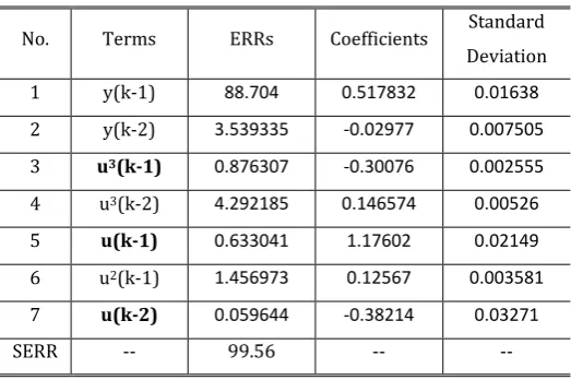
where v(k) is Gaussian noise v(k) ~ N(0,1). The AR process has a repeat pole at 0.8 and the coefficient 0.25 is chosen to guarantee the input signal is at a reasonable level. Here the noise signal e(k) is a Gaussian distributed noise with a variance 0.02, that is, e(k) ~ N(0,0.02). The results produced by the standard OFR algorithm are given in Table 1.

Table 1 Results produced by the standard OFR algorithm for example 1

No. Terms ERRs Coefficients Standard Deviation 1 y(k-1) 88.704 0.517832 0.01638

2 y(k-2) 3.539335 -0.02977 0.007505

3 u3_{(k-1) 0.876307 -0.30076 0.002555}

4 u3_{(k-2) 4.292185 0.146574 0.00526}

5 u(k-1) 0.633041 1.17602 0.02149

6 u2_{(k-1) 1.456973 0.12567 0.003581}

7 u(k-2) 0.059644 -0.38214 0.03271

SERR -- 99.56 -- --

Observe that two incorrect autoregressive terms were selected overwhelming the correct terms. A correct term u(k-1)u(k-2) was also missed in the identification. The new iterative orthogonal Forward regression algorithm which was introduced in the previous section was employed to overcome the problem by searching the optimal solutions on different paths. Combinations of any two terms in the model in Table 1 were selected as the pre-determined two terms and the remaining terms were selected in a model using a classic OFR algorithm. In this example, a total number of

( )

2

=

21

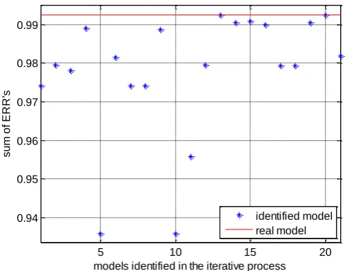
8 (7). This means the optimal model has been found on two different search paths. The optimal model is given in Table 2.

Fig 1 S ERR for example 1

Table 2 Model identified using the iOFR algorithm for example 1

No. Terms ERRs Coefficients Standard Deviation 1 u3_{(k-1) 63.77856 -0.30218 0.001013}

2 u(k-1) 27.00761 1.04567 0.02279

3 u (k-1)u(k-2) 8.084573 0.23962 0.002311

4 u(k-2) 0.370287 0.485927 0.02202

SERR -- 99.15 -- --

A reduction of the amplitude of the input causes a decrease of the signal-to-noise-ratio and consequently under these conditions the identification process may give an incorrect result. Consider an input given as

1 2

0.2

( ) ( )

1 1.6 0.64

u k v k

z- z

-=

- +

(9)

where v(k) is again a sequence of Gaussian noise v(k) ~ N(0,1).

The results of an iOFR process are given in Fig 2. It can be observed that some of the models give a larger SERR value than the correct model did. This means under this signal-to-noise-ratio level, any

5 10 15 20

0.94 0.95 0.96 0.97 0.98 0.99

models identified in the iterative process

su

m

o

f

E

R

R

's

9 system identification algorithm based on a RSS (residual sum of squares) criterion cannot produce a correct model.

F S ERR for example 1 with a small input

4.2 Example 2

Consider the following system.

 









 

2 2

1

0.5 1 0.8 ( 2) ( 1) 0.05 2 0.5 1

( ) ( )

1 0.5

w k w k u k u k w k

y k w k e k

z                _  (10)

The system was excited by an input defined as

1 2

0.16

( ) ( )

1 1.6 0.64

u k v k

z- z

-=

- + (11)

where v(k) is Gaussian noise v(k) ~ N(0,1). The AR process has a repeat pole 0.8 and the coefficient 0.16 is chosen so that the input signal has a similar amplitude as v(k). Here the noise signal e(k) is a Gaussian distributed noise with a variance 0.05, that is, e(k) ~ N(0,0.05). The results produced by the standard OFR algorithm are given in Table 3.

Table 3 Results produced by the standard OFR algorithm for example 2

No. Terms ERRs Coefficients Standard Deviation

1 y(k-1) 94.81906 0.680989 0.02521

2 y(k-2) 1.385184 -0.01539 0.02387

5 10 15 20

0.915 0.92 0.925 0.93 0.935 0.94 0.945 0.95 0.955 0.96

models identified in the iterative process

10

3 u2_{(k-1) 0.387782 1.48504 0.05909}

4 u(k-1)u(k-2) 1.483983 -0.81138 0.0719

5 u(k-1) 0.163537 0.5339 0.01987

6 y2_{(k-2) 0.546382 -0.03335 0.002269}

7 constant 0.230013 0.320967 0.02352

SERR -- 99.02 -- --

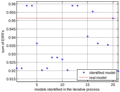
Observe that an incorrect autoregressive term y(k-2) was selected. Use two of the 7 terms in Table 3 as the previous term set and apply the new iOFR algorithm. Considering all the

( )

T SERR these models are shown in Fig 3 where the red line indicates the value of SERR of the correct model.

F S ERR for example 2

Fig 3 shows that 3 in 21 models gave the maximum SERR value which is equal to the SERR of the correct value. Actually all the three models are composed of the correct terms with same estimation of the associated parameters. The obtained model is shown in Table 4.

Table 4 Model identified using the iOFR algorithm for example 2

No. Terms ERRs Coefficients Standard Deviation

1 y(k-1) 94.81906 0.501414 0.01606

2 y2_{(k-2) 0.816735 -0.04615 0.001378}

3 u2_{(k-1) 0.899626 0.985615 0.01796}

4 u(k-2) 1.9376 0.769819 0.01552

5 10 15 20

0.98 0.982 0.984 0.986 0.988 0.99 0.992 0.994

models identified in the iterative process

su

m

o

f

E

R

R

's

11

5 constant 0.681966 0.494875 0.01951

SERR -- 99.15 -- --

4.3 Example 3

Consider system (12)

 









 

0.5 1 0.8 ( 2) ( 1) 0.05 2 0.5

y k  y k  u k u k  y k  e k (12)

with the input

1 2

0.16

( ) ( )

1 1.6 0.64

u k v k

z- z

-=

- +

(13)

where v(k) is Gaussian noise v(k) ~ N(0,1). The noise signal e(k) is a Gaussian distributed noise with a variance 0.05, that is, e(k) ~ N(0,0.05). The results produced by the standard OFR algorithm are given in Table 5.

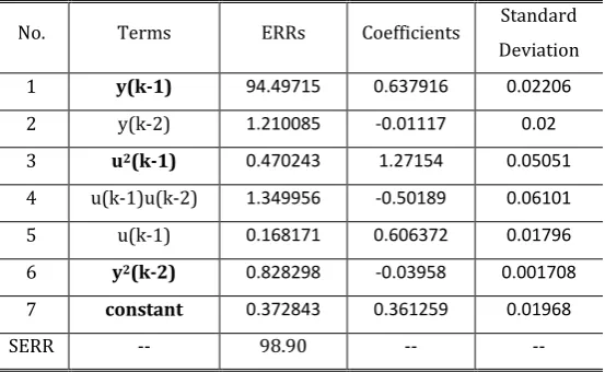
Table 5 Results produced by the standard OFR algorithm for example 3

No. Terms ERRs Coefficients Standard Deviation

1 y(k-1) 94.49715 0.637916 0.02206

2 y(k-2) 1.210085 -0.01117 0.02

3 u2_{(k-1) 0.470243 1.27154 0.05051}

4 u(k-1)u(k-2) 1.349956 -0.50189 0.06101

5 u(k-1) 0.168171 0.606372 0.01796

6 y2_{(k-2) 0.828298 -0.03958 0.001708}

7 constant 0.372843 0.361259 0.01968

SERR -- 98.90 -- --

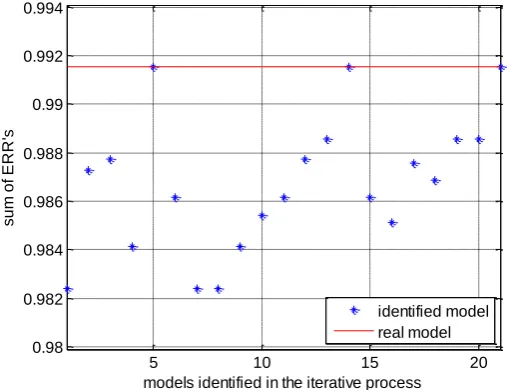
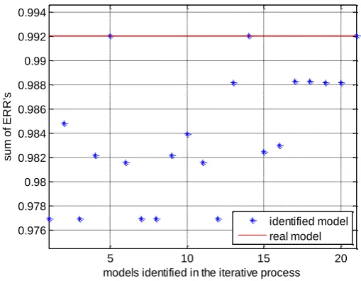
12 Fig 4 S ERR for example 3

Fig 4 shows that 3 in 21 models gave the maximum SERR which is equal to the SERR given by the real model (the red line in Fig 4). All the three models are of a correct model structure which is shown in Table 6.

Table 6 Model identified using the iOFR algorithm for example 3

No. Terms ERRs Coefficients Standard Deviation

1 y(k-1) 94.49715 0.491456 0.01157

2 y2_{(k-2) 0.503876 -0.04904 0.000997}

3 u2_{(k-1) 1.153346 1.00707 0.01419}

4 u(k-2) 2.178158 0.799251 0.0129

5 constant 0.87461 0.507799 0.01531

SERR -- 99.21 -- --

Notice that the coefficients given in Table 6 are more accurate than the estimates given in Table 4. This happens because the noise affects systems (10) and (12) in a different way though both systems are of the same structure except for the noise models. In system (10) the output was corrupted by observation noise which does not involve the dynamics of the system. In contrast, system (12) was corrupted by process noise which affects the whole process of the system.

5. Conclusions

5 10 15 20

0.976 0.978 0.98 0.982 0.984 0.986 0.988 0.99 0.992 0.994

models identified in the iterative process

su

m

o

f

E

R

R

's

13 A new iterative forward orthogonal regression algorithm has been used to solve the suboptimal problem caused by non-persistent excitation. By slightly revising the classic OFR algorithm, the new iOFR algorithm is much more robust to non-persistent inputs. Examples showed that the new iOFR algorithm is capable of correctly identifying the models and gives the optimal result when the noise-to-signal-ratio is at a reasonable level.

The new iOFR algorithm, which works under a purely OFR-ERR spirit, inherits the advantages in computational efficiency and universal applicability. The new iOFR algorithm provides a robust and efficient choice for the application of nonlinear system identification in real systems where the inputs cannot be optimally designed.

Acknowledgements

The authors gratefully acknowledge support from the UK Engineering and Physical Sciences Research Council (EPSRC) and the European Research Council (ERC).

References

BILLINGS, S. A. (2013) Nonlinear system identification : NARMAX methods in the time, frequency, and spatio-temporal domains, John Wiley & Sons Ltd.

GUO, Y., GUO, L. Z., BILLINGS, S. A. & WEI, H. L. (2014) A new iterative orthogonal forward regression algorithm. Intern. J. Syst. Sci., submitted.

HIRSCH, M. D. R., LUIGI (2010) Iterative Identification of Polynomial NARX Models for Complex Multi-Input Systems. IN MARCONI, L. (Ed.) 8th IFAC Symposium on Nonlinear Control Systems. University of Bologna, Italy.

HJALMARSSON, H. & MARTENSSON, J. (2007) Optimal Input Design for Identification of Non-linear Systems: Learning From the Linear Case. American Control Conference, 2007. ACC '07. LARSSON, C. A., HJALMARSSON, H. & ROJAS, C. R. (2010) On optimal input design for nonlinear

FIR-type systems. 49th IEEE Conference on Decision and Control (CDC).

LEONTARITIS, I. J. & BILLINGS, S. A. (1985) Input-output parametric models for non-linear systems Part I: deterministic non-linear systems. International Journal of Control, 41, 303-328.

LJUNG, L. (1987) System Identification: Theory for the User, Englewood Cliffs, N.J., Prentice-Hall, Inc. MAO, K. Z. & BILLINGS, S. A. (1997) Algorithms for minimal model structure detection in nonlinear

dynamic system identification. International Journal of Control, 68, 311-330.

NARENDRA, K. S. & ANNASWAMY, A. M. (1984) Persistent Excitation in Dynamical Systems. American Control Conference, 1984.

NOWAK, R. (2002) Nonlinear system identification. Circuits, Systems and Signal Processing, 21, 109-122.

PIRODDI, L. & SPINELLI, W. (2003) An identification algorithm for polynomial NARX models based on simulation error minimization. International Journal of Control, 76, 1767-1781.

S̈DERSTR̈M T System Identification, New York; London, Prentice Hall.