Use of a novel dataset to explore spatial and social variations in car type, size, usage and emissions

Use of a novel dataset to explore spatial and social variations

in car type, size, usage and emissions

Tim Chatterton

, Jo Barnes

, R. Eddie Wilson

, Jillian Anable

, Sally Cairns

University of the West of England, UK b

University of Bristol, UK c

University of Aberdeen, UK d

Transport Research Laboratory, University College London, UK

a r t i c l e

i n f o

Keywords: Emissions Vehicle Energy Household Spatial

Socio-demographic

a b s t r a c t

The ’MOT’ vehicle inspection test record dataset recently released by the UK Department for Transport (DfT) provides the ability to estimate annual mileage figures for every indi-vidual light duty vehicle greater than 3 years old within Great Britain. Vehicle age, engine size and fuel type are also provided in the dataset and these allow further estimates to be made of fuel consumption, energy use, and per vehicle emissions of both air pollutants and greenhouse gases. The use of this data permits the adoption of a new vehicle-centred approach to assessing emissions and energy use in comparison to previous road-flow and national fuel consumption based approaches. The dataset also allows a spatial attribution of each vehicle to a postcode area, through the reported location of relevant vehicle testing stations. Consequently, this new vehicle data can be linked with socio-demographic data in order to determine the potential characteristics of vehicle owners.

This paper provides a broad overview of the types of analyses that are made possible by these data, with a particular focus on distance driven and pollutant emissions. The inten-tion is to demonstrate the very broad potential for this data, and to highlight where more focused analysis could be useful. The findings from the work have important implications for understanding the distributional impacts of transport related policies and targeting messaging and interventions for the reduction of car use.

Ó2015 The Authors. Published by Elsevier Ltd. This is an open access article under the CC BY license (http://creativecommons.org/licenses/by/4.0/).

Introduction

Efforts to reduce greenhouse gases in the UK are regularly framed in terms of the overall ‘legally binding’ commitment for an 80% reduction in greenhouse gas emissions relative to 1990 levels that is set out in the 2008 Climate Change Act. 24% of current domestic UK GHG emissions are from transport (DECC, 2013). Car travel contributes 58% of this, whilst light vans contribute 12.5% and motorbikes/mopeds contribute 0.5% (DfT, 2011). Due to the inability of some source sectors to make an 80% reduction, such as agriculture, waste and domestic aviation, it will be necessary for other sectors, particularly domes-tic surface transport, to decarbonise almost entirely (Committee on Climate Change, 2010; DECC, 2011). In addition to the problem of greenhouse gases and climate change, road transport is responsible for over 95% of the Air Quality Management

http://dx.doi.org/10.1016/j.trd.2015.06.003

1361-9209/Ó2015 The Authors. Published by Elsevier Ltd.

This is an open access article under the CC BY license (http://creativecommons.org/licenses/by/4.0/).

⇑Corresponding author at: Air Quality Management Resource Centre, Faculty of Environment and Technology, University of the West of England, Bristol BS16 1QY, UK. Tel.: +44 (0)117 328 2929.

E-mail address:[email protected](T. Chatterton).

Contents lists available atScienceDirect

Transportation Research Part D

Areas declared under the UK’s Air Quality Strategy and Local Air Quality Management (LAQM) framework (Longhurst et al., 2011).

This paper sets out how new data released by the UK Department for Transport (DfT) can offer a radically new perspective on these emissions, and on energy use, through calculations at the level of the individual vehicle. The data is acquired from the UK annual road worthiness vehicle inspection data (known as the ‘MOT (Ministry of Transport) test’)1_{which provides}

information on vehicle characteristics, annual mileage and the (presumed) location of the vehicle owner (via the location of the Vehicle Test Station – see below). By attributing energy and emissions across the country to a relatively local level, based upon actual vehicle mileages, the methodology set out in this paper offers completely novel calculations that have been impos-sible to date. Although there is existing work that links energy use and emissions to household location (see for example

Hatzopoulou et al., 2007, 2011), the methodologies used in these studies employ modelled trip data and have only been under-taken at the level of individual cities. The point of the methodology set out in this paper is not to presume that vehicles are driven at the point of registration or VTS, but instead to link fuel use and emissions to vehicle ownership.

In addition, by linking the MOT data spatially with socio-demographic data, it is possible to work towards an assessment ofwhois responsible for energy and emissions (in terms of area of residence and general demographic characteristics), rather thanwhythey are emitted (e.g. journey purpose – see, for example,DfT (2008), Chapter 3) or source calculations ofwhere

they are emitted (e.g. emissions calculations based on flows for road links, as used in the UK National Atmospheric Emissions Inventory – seeWaygood et al. (2013)for a short description of the NAEI and similar methodologies). Whilst the spatial loca-tion of greenhouse gas emissions, unlike ‘convenloca-tional’ air pollutants, is largely immaterial in terms of ambient concentra-tions due to the global nature of climate change (seeTiwary et al., 2013), it is relevant to climate mitigation policy in order to identify emitters and appropriately target reduction measures. Spatial location of vehicle owners is also relevant with regard to energy use where, in a future when Plug-In Vehicles may have become established, the majority of energy required by the Light Duty Vehicle (LDV) fleet may need to come from the local electricity distribution grids of the owners rather than in liquid/gas form from filling stations.

The use of local data, linking emissions to location of vehicle owners, allows links to be made between responsibility for emissions and exposure to local-scale public health and environmental problems. This need not be limited just to the con-sideration of conventional air pollutants as done here (particulate matter (PM) and nitrogen oxides (NOx)) but could be extended to other public health issues associated with car use such as noise, road safety, and use of public space for which distances driven can be seen as a proxy variable. The approach also affords a new method for assessing environmental and social justice issues around air pollution, building on work such asMitchell and Dorling (2003). In particular, this work high-lights the difference between apotentiallydirty car (i.e. one with high emissions or fuel consumption per km) and anactually

dirty car (i.e. based on total emissions from the vehicle in any given per year).

This paper demonstrates the potential value and diversity of analyses afforded by the MOT dataset, including estimations of commonly used statistics (e.g. vehicle km/year for private vehicles) but from a novel data source. A review of vehicle inspection and maintenance programmes (Cairns et al., 2014) has indicated the extent to which these tests are carried out globally, and therefore the potential for the work presented here to be carried out elsewhere. Since 31st December 2011, all 27 European Member states (under European Directive 2010/48/EU) are required to undertake vehicle inspection tests at least every two years (once vehicles are four years old or over). In the US, 17 states have compulsory periodic (annual or biennial) safety inspection programmes, whilst 32 states have either partial or full emissions inspection programmes (Wikipedia, 2015). In Asia at least 17 countries were testing for roadworthiness and/or emissions (UNEP, 2011a). Although vehicle inspection data have been used for certain types of analysis previously, to date, we are not aware of any similar work of the scale and nature described here, although, given the widespread nature of such testing, there is considerable potential for such work.

Data description and methodology

The MOT dataset

In 2010, DfT began publishing results from the annual MOT tests. Around 38 million test records (including test passes and test failures) relating to some 27 million vehicles are stored in the database each year (DfT, 2013a). With the application of some mathematics (see, for example,Cairns et al., 2013; Wilson et al., 2013a, 2013b), it is possible to estimate the annual distance driven for the majority of LDVs in the UK.2_{DfT have undertaken some analysis of this dataset focussing primarily on}

vehicle age and mileage (DfT, 2013a). In addition to the odometer reading of the vehicle at each test, the dataset includes details of the make and model of the vehicle, engine size, fuel type, date of first registration and colour. The primary unit in the current public release of the data is the vehicle test (rather than the vehicle). Each test (and therefore the vehicle undergoing the test) is spatially attributed to the Postcode Area (PCA – see below) of the relevant Vehicle Testing Station (VTS) where the vehicle

1

http://data.gov.uk/dataset/anonymised_mot_test. 2

inspection is carried out (DfT, 2014a). The VTS location can therefore be used as a proxy for the location of the vehicle owner in the absence of any other locational information. Key caveats around this data are:

The location of the VTS is not an ideal proxy for the location of the owner of the vehicle. People are able to take their car to any testing station, however due to rules regarding where and how failed vehicles can be retested (Gov.uk, 2015) there is a reasonable likelihood that people will have their cars tested at a testing station close to their home. Moreover, the prob-ability that the VTS and home location both fall within a PCA is relatively high, given that PCAs are relatively large (see below).

The dataset does not include the majority of vehicles <3 years of age as these are not currently required to undergo an annual MOT test.3Around 13% of all cars in the UK fleet were estimated to be under 3 years old (DfT, 2014b). Work is cur-rently being undertaken to identify and utilise additional datasets to improve the knowledge of these – although it should be noted that many of these vehicles will be owned by rental or leasing fleets, or individuals with a strong preference for new vehicles – and may therefore have atypical usage patterns.

Vehicles disappear from the dataset after their last test, so an unknown distance is driven between a vehicle’s last test and when it is scrapped or taken off the road. Exact details of how many vehicles are actually taken off the road and scrapped each year are surprisingly hard to obtain, but estimates indicate it is usually somewhere between 1 and 2 million (Car Recycling, 2012)

A certain number of vehicles will not have an MOT test and will therefore be driven on the roads illegally. Due to the increasing computerisation of the system, this is a decreasing number. The Driver and Vehicle Licensing Authority (DVLA) carry out annual number plate surveys which estimate the scale of this problem to be small. Only 0.6% of vehicles, around 210,000, were calculated to be unlicensed in 2013, and those without valid MOT certificates are a subset of this (DfT, 2013b).

The current dataset contains a range of vehicle types, including cars, Light Goods Vehicles <3.5 tonnes (LGVs), motorbikes and private buses. Our analysis has not differentiated between different vehicle types – instead, variance in engine size is considered as an important differentiator.

The dataset used is from the September 2013 release (VOSA, 2013). Following processing of the data, information was available for 24,391,789 individual vehicles, including an estimate of the annual distance driven by each in 2012.

Calculating emissions and energy use

Per kilometre emissions and energy use are calculated here as an outcome of three key variables from the MOT dataset: date of registration (indicating likely pollution control technologies), engine size, and fuel type (impacting on both fuel econ-omy4_{and emissions). These are then multiplied by the calculated annual distance travelled in order to estimate annual}

emis-sions and energy usage for each individual vehicle.

The MOT dataset categorises vehicles according to fuel type under the classes: Petrol, Diesel, Liquefied Petroleum Gas (LPG), Liquefied Natural Gas (LNG), Compressed Natural Gas (CNG), Steam, Fuel Cell, and Other. For the purposes of this anal-ysis, steam-powered vehicles have been removed and, following examination of make/model information, ‘Fuel Cell’ and ‘Other’ have been grouped together and treated as Hybrid (petrol electric). Due to the very small proportion of ‘alternative fuel vehicles’ (i.e. vehicles which are not petrol or diesel), the spatial presentation of fuel type has focussed on the proportion of diesel vehicles for each PCA.

In terms of the relative environmental impacts of petrol and diesel vehicles, although diesel vehicles have been heavily incentivised by UK national and local government policies (i.e. Vehicle Excise Duty and the congestion charge) on the basis of lower CO2emissions, the higher emissions of PM from diesel engines lead to increased short-term warming and significantly

higher human health impacts compared to petrol (Uherek et al., 2010; UNEP, 2011b).Table 1shows recent figures (Defra, 2010) which found that monetisation of these impacts indicates monetised equivalence in the combined air quality and cli-mate impacts between petrol and diesel cars, highlighting the importance of considering both greenhouse gases and conven-tional air pollutants.

No account has been taken in this analysis of differentiation between vehicle types (e.g. car, LGV, two-wheeler). Initial attempts were made to manually categorise the vehicles using appropriate vehicle classes, including sub-groupings (e.g. ‘city-car’, ‘saloon’, etc.) but this has proved impractical with over 33,000 unique combinations of make and model within the dataset. Provision of an indicator of ‘body type’ in future data sets will allow better treatment of this. It is also anticipated that future releases of the data may also include vehicle manufacturers’ values for emissions and fuel economy which will allow for an assessment of uncertainty to be made with regard to the calculations presented here. However, it is of note that numerous studies show that manufacturers’ reported emissions do not accurately reflect in-use emissions (e.g.Carslaw et al., 2011; Mellios et al., 2011; Sileghem et al., 2014).

3

In the DfT data release in September 2013, <0.1% of vehicles listed were less than three years old (i.e. registered in 2010–12). 4

Emissions and energy use have been calculated on the basis of vehicle age, fuel type, engine size and derived km/year. All cars reported as ‘Fuel Cell’ or ‘Other’ have been treated as petrol hybrids. Steam vehicles have been discounted from the anal-ysis (n= 62). There has been a mis-attribution of hybrid vehicles to other fuel types (including steam,n= 14) which has been possible to partially identify by searching for ‘‘PRIUS’’. This highlights some potential issues with the data quality which merit further attention. However it has been impractical in this exploratory work to focus on identifying these misclassifi-cations and calculations have been based on engine size and fuel type as stated.

Emissions of NOx, PM10and CO2have been calculated from a set of generic emission factors developed by the Air Quality

Management Resource Centre at the University of the West of England (Barnes and Bailey, 2013). These are based on the currently best available data for the UK from a range of sources (primarily COPERT 4 (v8.1) (Ntziachristos et al., 2009),

TRL (2009), NAEI (2013a)and EMEP/EEA (EEA, 2013)). The emission factors for NOx, PM10and CO2used were for cars of

dif-ferent fuel types: Petrol (<1400 cc, 1400–2000 cc, and >2000 cc: Pre-Euro and Euro 1–6), Diesel (<2000 cc and >2000 cc: Pre-Euro and Euro 1–6), LPG (all engine sizes: Euro 1–6 (pre-Euro 1 treated as Euro 1)), Hybrid (single factor). These emission factors were available for urban, rural and motorway driving. A compound emission factor was calculated based on figures from Transport Statistics Great Britain (DfT, 2012) that split total mileage for cars, motorbikes and LGVs between motorways (19%), urban (28%) and rural (43%). Euro standards for the vehicles have been based on date of first registration in relation to the EU compliance date for the relevant standards (seeTable 2). As described above, due to the absence of data on body type, all vehicles have been treated as cars.

Due to a lack of information on emission factors for light duty CNG and LNG vehicles, NOx and PM10emissions for these

were based on LPG, by km travelled. CO2emissions from LNG were also set on the basis of LPG. However, CO2emissions for

CNG were calculated on a g/l basis, given the significantly different volume:energy ratio due to the compressed nature of the fuel. This is described below. Details of final emissions factors for each fuel type are given inTable 3.

Fuel economy and fuel consumption calculations

Fuel economy figures for petrol and diesel vehicles were derived from data for Ireland (CSO, 2013) due to the likely sim-ilarity of the vehicle fleet and the quality and availability of the data, which gives average fuel economy figures for petrol and diesel vehicles sold between 2000 and 2011 breaking vehicles down into 100 cc bands between 900 cc and 3000 cc. Similar data was sought for the UK, however, government guidance (WebTAG) on calculating fuel consumption only provides data for fuel consumption for cars split into petrol car/diesel car (DfT, 2014c) with no distinction between engine sizes, and

ret-Table 1

Typical annual environment and health cost of car travel (Defra, 2010).

Costs with regard to: Petrol car Diesel car Petrol hybrid

Climate change £166 £146 £98

Air quality £1 £21 £1

Total £167 £167 £99

Table 2

Dates for introduction of Euro standards for cars/LDVs.

Euro1 Euro2 Euro3 Euro4 Euro5 Euro6

Cars July 1992 Jan 1996 Jan 2000 Jan 2005 Sept 2009 Sept 2014

LDVs Oct 1994 Jan 1998 Jan 2000 Jan 2005 Sept 2009 Sept 2014

Table 3

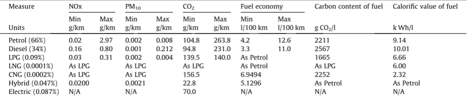
Emission factors, fuel economy and calorific values used for all fuel types.

Measure NOx PM10 CO2 Fuel economy Carbon content of fuel Calorific value of fuel

Min Max Min Max Min Max Min Max

Units g/km g/km g/km g/km g/km g/km l/100 km l/100 km g CO2/l k Wh/l

Petrol (66%) 0.02 2.97 0.002 0.008 104.8 263.8 4.2 12.6 2211 9.14

Diesel (34%) 0.16 0.80 0.001 0.212 94.8 231.0 3.3 11.0 2567 10.01

LPG (0.09%) 0.03 0.31 0.002 0.004 139.5 140.0 As Petrol 1665 6.66

LNG (0.0001%) As LPG As LPG As LPG As Petrol As LPG 6.00

CNG (0.0002%) As LPG As LPG 156.5 6.9494 2252 2.32

Hybrid (0.047%) 0.0200 0.0021 22.8 5.1296 As Petrol As Petrol

Electric (0.087%) N/A N/A 70.0 N/A N/A N/A

rospective changes in fuel efficiency, and with data only going back as far as 2004. All vehicles registered before 2000 were treated as 2000, which may lead to some bias from underestimating older vehicles, however <15% of the vehicles in the data-set were registered before 2000. It is anticipated that future work with an improved datadata-set will enable further analysis of this ‘old vehicle’ subset. It is recognised that there may be significant differences in vehicle purchasing patterns between the UK and Ireland, and further work is planned to validate and improve these initial assumptions and will be aided by the antic-ipated addition of manufacturers’ figures within future releases of the MOT dataset.

Due to lack of suitable fuel economy figures for LPG and LNG vehicles, these have currently been set as for petrol, although usually LPG is 5–10% less efficient. Fuel economy for CNG vehicles has been calculated by taking an average g CO2/km from

the two CNG vehicles on the carfueldata.gov website (VCO, 2013) of 156.5 g CO2/km. On the basis that the carbon content of

1 l of CNG is emitted as 2252 g CO2(Ecoscore, 2013), the fuel use of CNG vehicles has been estimated at 6.95 l/100 km. Fuel

economy for hybrids has been calculated by taking an average 122.7 g CO2/km from the 70 hybrid vehicles on the

carfuel-data.gov website (VCO, 2013) and, on the basis that 1 l of petrol emits 2211 g CO2(DfT, 2014d), fuel use of hybrids is

esti-mated as 5.55 l/100 km. These fuel economy figures of l/100 km were then multiplied by the estiesti-mated annual vehicle mileage to generate fuel consumption figures – specifically, a figure of litres of fuel per year for each vehicle. Details of figures for fuel economy for each fuel type are given inTable 3.

As with any estimation of vehicle emissions, these calculations represent a notional value that, irrespective of details such as the bandings of engine size, can only ever loosely reflect precise in-use emissions which will depend on a variety of factors such as power/acceleration, engine temperature and engine condition. However, the most representative figures available for in-use emissions and fuel economy have been used. Future work will try to improve these further and, should they become available in future releases of the dataset, will utilise manufacturers’ emission and fuel economy figures. It is also acknowledged that whilst the current approach varies emissions of pollutants for vehicles based on a provisional urban/rural/motorway split, this has not been possible for fuel consumption and therefore energy usage (nor for CO2

emis-sions for CNG or hybrid vehicles). It is hoped that further improvements to the dataset in future releases may include further information on these.

Energy use calculations

Energy use of all vehicles, other than electric, has been calculated on the basis of UK Department for Environment, Farm-ing and Rural Affairs (Defra) Greenhouse Gas ReportFarm-ing Guidelines (Defra, 2013a). These provide the calorific value for all relevant fuels (kW h/kg) along with a density (l/tonne) from which a calorific value of kW h/l was calculated. This was then multiplied by the fuel used per year to estimate total energy usage per vehicle. Electric vehicle energy use was set at 0.211 kW h/km with CO2emissions of 70 g/km (Wilson, 2013), however no emissions of PM or NOx were attributed for

these.

Postcode areas (PCAs)

The vehicle data presented in this paper are primarily attributed to Postcode Areas (PCAs), the largest geographical post-code domain which splits Great Britain (GB) into 120 unequal areas. Within the process set out in earlier work (Cairns et al., 2013; Wilson et al., 2013b), each calculation of annual mileage for a vehicle results in two PCAs being attributed per vehicle, one for the first test and one for the second. Within this paper, the final (second) PCA has been used to represent the location of the vehicle (for over 19 million (80%) of the 24.4 million vehicles, the first and second PCA were the same). Environmen-tal impacts (pollution emissions and energy use) are calculated for each individual vehicle in the MOT dataset and then aver-aged over each PCA to provide an indication of the average vehicle characteristics for each area. We recognise that this level of spatial aggregation may be considered too large to derive a valid depiction of an average vehicle on which to determine meaningful relationships with socio-economic data over the same areas. However, we present this as exploratory work, set-ting out a range of possible analyses as a proof-of-concept. We acknowledge not only the limitations that this spatial reso-lution brings, but conversely the advantages associated with the initial presentation and analysis of the spatial data for Great Britain divided over only 120 PCAs as opposed to tens of thousands of smaller spatial areas such as census Lower-layer Super Output Areas (LSOAs). Within the data presented below, there is a clear indication of patterns that merit further research and exploration at a depth that is impossible within a single paper. To aid readers unfamiliar with the geography of Great Britain,

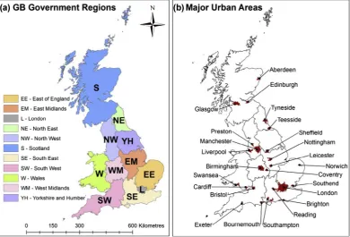
Fig. 1shows key urban areas and regions that will be useful in interpreting the analysis and results.

Table 4provides descriptive information highlighting the varied nature of PCAs. As discussed above, PCAs are often very large and, unlike census geographies, have not been defined to represent socially homogeneous populations. The PCA bound-aries are used to present results in various maps produced below, such asFig. 2.

Statistical approach

Results

Spatial variations and relationships in key vehicle parameters

Five key parameters have been taken for each vehicle in the MOT dataset for 2012 and then a mean calculated for each PCA to represent an ‘average vehicle’. These parameters are:

Odometer reading:The odometer reading from the second test provides an indication of the total distance driven by the vehicle over its lifetime. This could be taken as a proxy for wear and tear in addition to vehicle age, but only accounts for how far a vehicle has been driven, not how hard it has been driven or how well it has been maintained.

Engine size:The average engine size (in cc) taken from the MOT record. These have been screened to exclude obviously erroneous recordings for engine sizes above 9000 cc. As described above, for the fuel consumption calculations, there are 100 cc bins for all vehiclesP900 cc and63100, and single bins for all vehicles below or above these sizes.

Vehicle age:This is taken to be the number of years between 2012 (the year of the ‘straddling date’ used to estimate cal-endar year annual distance driven) and the year of first registration.

Annual distance driven per vehicle (km driven):This is the estimated annual distance driven calculated from the interval between vehicle test results. A straddling date of 1st July 2012 has been set to represent vehicle usage for the calendar year 2012.

Fuel economy:Although this data is not (currently) available within the MOT dataset itself, this has been calculated for each vehicle as described above, and has been included within these parameters as a vehicle characteristic, and not an energy or emission outcome. As described above, the fuel consumption calculations treat pre-2000 as 2000, and so there is likely to be an underestimation of fuel consumption of older vehicles.

Fig. 1.Maps showing GB government regions and major urban areas.

Table 4

Characteristics of 120 GB postcode areas.

Minimum Mean Maximum

Area (km2

) 3.4 1552 6433

Households (2011) 613 219,754 821,717

Population (2011) 1553 559,022 2,191,953

Population density (p/km2

) 0.24 1501 15,878

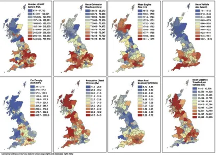
The spatial variation in the mean values for these parameters by PCA are presented inFig. 2alongside three further val-ues: the number of ‘cars’ in each PCA, the density of ‘cars’ per km2_{, and the proportion of diesel vehicles within the PCA.Fig. 3}

presents bivariate scatterplots for six of these parameters indicating the varying relationship between them (including linear regression lines andRvalues calculated in the statistics package R (R Core Team, 2012)).

From the data presented inFigs. 2 and 3, a number of patterns can be seen. These are described below in relation to the regions and urban areas shown inFig. 1.

Density of vehicles is greatest around the main conurbations (London, Birmingham, Cardiff, Liverpool, Brighton, Southampton, etc.).

Vehicles with highest odometer readings are mainly in the East of England, Wales, West and East Midlands and the South West.

Engine size is greatest in northern Scotland, the South East and mid-Wales.

The oldest vehicles are in the East of England, the South West and South Coast (including South East and South West).

The greatest proportions of diesel vehicles are in Wales, northern and southern Scotland (but not central Scotland near Edinburgh and Glasgow) and the South West. As might be expected, the relationship between fuel economy and the per-centage of diesel vehicles is negative (R= 0.65).

Fuel economy of vehicles (l/100 km) is worst in South East England and in Scotland around Aberdeen.

Greatest mean annual distance driven per vehicle is in northern and southern Scotland, the northeast of England, and an area in central England where the East and West Midlands, and the East and South East of England meet. Places with higher annual per vehicle distance also tend to have better fuel economy (R= 0.56).

The strongest relationship is between engine size and fuel economy (R= 0.75), which has a stronger relationship than vehicle age and fuel economy (R= 0.47).

As the purpose of this paper is to demonstrate the potential for this dataset to reveal patterns of interest rather than to undertake detailed analyses, we do not go into these further here. However, all these points merit far more analysis than is possible within this paper.

Spatial variations in emissions and energy consumption

As with the key vehicle parameters above, annual emissions for NOx, PM10and CO2have been calculated for each

indi-vidual vehicle before deriving the mean value for each PCA.Fig. 4shows the spatial variations in these. The highest values across both sets of pollutants tend to be in northern and southern Scotland (but not the ‘central belt’ containing the main Scottish conurbations (Edinburgh and Glasgow)) and an area in central England where the East and West Midlands, and the East and South East of England meet. Wales and the South West have higher relative emissions of NOx and PM10than

they do emissions of CO2and energy consumption. Analysis of the relationship between the variables shown in this figure,

conducted on a similar basis to that reported above, shows that emissions of NOx and PM10are strongly correlated (R= 0.99),

as are CO2and energy consumption (R= 0.99). NOx and PM10are less well correlated with CO2and energy, although there is

still a strong correlation, withRvalues between 0.74 and 0.81.

Determinants of average CO2emissions

Fig. 5shows the bivariate relationships between the mean vehicle CO2emissions and eight key vehicle parameters for

each PCA. For the purpose of this paper, CO2has been chosen as being, to some extent, illustrative of all emissions and energy

use given the strong relationships demonstrated above. Again, it should be noted that this paper provides an overview of the data and spatial differences in the means of these parameters. Further work is justified in exploring the variance and rela-tionships between these parameters at the level of individual vehicles. However, some interesting points can be noted:

The strongest relationship is between average CO2 per vehicle and average annual distance driven per vehicle (km

driven) – indicating that in terms of environmental impacts, it is not necessarily the type of car that is important but the distance travelled, at least at this level of spatial aggregation.

Fig. 3.Relationships between mean vehicle parameters by PCA (Rvalues are presented in upper panel diagonally opposite the relevant plots, along with indicators of significance⁄

p< 0.05,⁄⁄

CO2emissions per vehicle appear to increase with the proportion of diesel vehicles in the PCA. This is counter-intuitive

given that diesel vehicles tend to have lower emissions per distance travelled. However, it appears that this may be because, due to better fuel economy, diesel vehicles are often driven further than petrol vehicles. Again, further analysis at the level of individual vehicles may reveal more about this.

Vehicle age in years is only weakly correlated with CO2. However, the further the vehicle has been driven over its lifetime,

i.e. the total distance on the odometer, the higher the annual CO2emissions (R= 0.61). This suggests that there are

com-plex factors relating historical distances driven with distance travelled in the current year.

As average fuel economy worsens (l/100 km increases), average CO2 emissions decrease. This initially appears

counter-intuitive, but is likely to be because less economic vehicles are driven shorter distances.

At the aggregate level, average engine size is not clearly related to average emissions of CO2, and this is likely to be due to

a combination of historical distance driven, vehicle age, fuel type and, most importantly, average distance driven exerting a much stronger influence on these emissions.

To further explore the complex relationships underlying these parameters, a further analysis was undertaken using mul-tiple regression usingR. The eight parameters illustrated inFig. 5were put into a multiple regression model and analysed in a stepwise manner to produce a minimal adequate model, retaining parameters on the basis of significance (p< 0.001). Engine size was discarded due to poor significance of its bivariate relationship (seeFig. 5). This poor relationship may be due to the tendency for diesel vehicles, which emit less CO2per km, to have larger engines than equivalent petrol vehicles.

Fig. 4.Spatial variation in mean annual emissions and energy use per vehicle.

The stepwise process also led to the rejection of the number of cars per PCA, the percentage of diesel vehicles per PCA, and the odometer reading on the basis of poor significance.

The remaining variables were then tested for collinearity by examining variance inflation factors (VIF). The VIFs were all less than 3, indicating acceptable levels of collinearity. Key statistics for the regression model are given inTable 5. The overall

R-squared value for the model, showing goodness of fit, is extremely high at 0.9981. This is due, at least in part, to the strong relationship between km driven and CO2. Notably, in this model, all parameters are showing a positive relationship with CO2

(unlike in the bivariate analysis). A further model run, excluding the km driven parameter, produced anR-squared value of only 0.2691, indicating the over-riding significance of this variable.

Relationships between vehicle type, emissions and socio-demographic data

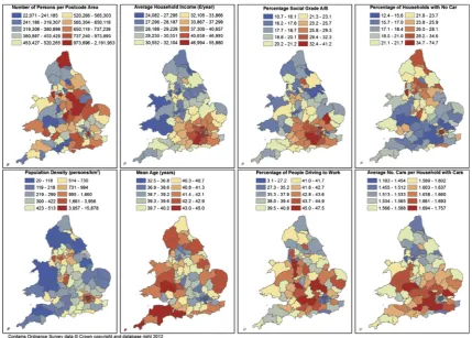
Not only can the spatial attribution of data help to identify the general geographical location of the owners of vehicles generating relatively high levels of emissions or energy consumption, but it can be combined with data from the census (and other sources) to identify a picture of the average socio-demographic profile of the populations likely to be responsible for these vehicles.Fig. 6shows eight key socio-demographic parameters. Six of these have been taken directly from the 2011 Census (ONS, 2011): number of persons per PCA, mean age, percentage of households containing a ‘Household Reference Person’ of social grade AB (i.e. employed in higher & intermediate managerial, administrative or professional occupations),

Table 5

Regression results for influence of vehicle parameters on CO2.

b Beta Std. error t p

(Intercept) 1.098 0.033 33.35 <0.001

km driven 1.54E 04 1.117 7.38E 07 208.26 <0.001

Fuel economy 0.133 0.175 0.005 29.17 <0.001

Vehicle age 0.016 0.065 0.001 13.34 <0.001

Car density 6.68E 06 0.022 1.68E 06 3.98 <0.001

R-squared = 0.9981.

percentage of households with no access to a car, average number of cars per household (for those households with a car), and percentage of workers driving to work. Population density has been calculated from the PCA area and total census pop-ulation. Average income has been calculated using a median household income figure obtained from Experian, a private busi-ness data provider (Experian, 2011). All data has been aggregated upwards from data for Lower-layer Super Output Areas. As with the aggregation of the vehicle parameters, the intention is to provide an indication of the average qualities of an area, rather than making statements about what any individual person/household may be like (and therefore risk ecological fal-lacy). Due to differences in census data collection and geographies for Scotland, socio-demographic data have currently only been analysed for England and Wales.

As with the plots inFig. 3, bi-variate relationships have been investigated between these parameters. However, as the focus of this paper is on demonstrating the use of the MOT dataset and not the socio-demographic patterns these are not presented here. The most notable feature, though, is that each of these variables is also significantly spatially variant, and the patterns of variance do not necessarily correspond with those shown inFig. 2for vehicle parameters.

Fig. 7shows the relationships between both mean km driven per vehicle for each PCA, and the eight socio-demographic characteristics shown inFig. 6. Due to the strong correlations between average km driven per vehicle and CO2, energy

con-sumption, NOx and PM10(described above) the similar plots for the other outcome parameters have not been presented

here.

Four socio-demographic parameters were found to have strong correlations (R> 0.6). The percentage of people who drive to work, and the mean number of cars per household were both found to have strong positive correlations. Population den-sity and the percentage of households with no access to a car were found to have strong negative correlations. Moderate correlations (RP0.3 and6_{0.6) were found for mean age (positive), household income and percentage of households in social}

grade AB (both negative). There was no significant (p< 0.05) correlation found with the population of the PCA.

These eight parameters were then put into a multiple regression model and parameters discarded in a stepwise fashion on the basis of significance (p< 0.001). This resulted in only income, age and the percentage of households with no car remaining. Regression statistics are shown inTable 6. These indicate that the average distance travelled by each vehicle in each PCA decreases with both income and age, and increases as more households own a car. Together these explain

Fig. 7.Relationship between average km driven per vehicle and average socio-demographic characteristics (HH = Household).

Table 6

Regression statistics for average distance travelled per vehicle as a function of socio-demographic parameters.

b Beta Std. error t p

(Intercept) 24330.00 1763 13.804 <0.001

% Households with No car 83.12 0.91 7.284 11.412 <0.001

Income (median) 0.08 0.58 0.009 8.438 <0.001

Age (mean) 201.20 0.50 36.33 5.537 <0.001

66% of the variation in the mean distance travelled by vehicles for each area. The importance of the proportion of households without (or with) a car may reflect the general accessibility characteristics or car dependency of the area, i.e. where a higher proportion of households do not own cars, it is likely that those households which do own cars need tousethem less to access services.

Linking to air pollution emissions and exposure

In addition to socio-demographic data, it is also possible to analyse the MOT data in relation to environmental datasets, such as air pollution emissions from road transport and levels of exposure to air pollutants, for which are available for the whole of the UK as a 1 km2 _{resolution grid (Defra, 2013b; NAEI, 2013b). This type of analysis might present interesting}

opportunities in relation to improving aspects of emissions inventory construction (e.g. variations in the significance of addi-tional cold start emissions based on residential location), as well as investigating issues of social and environmental justice regarding relationships between responsibility for emissions and exposure (c.f.Mitchell and Dorling, 2003). Such work would be improved given better spatial resolution for the MOT dataset. An initial comparison of total emissions for road transport from the NAEI (aggregated to PCA level), and total emissions from the vehicles in the MOT dataset for each area show very strong correlations (R= 0.96–0.98), despite being based on completely different methodologies (road flows vs. individual vehicles). This strongly suggests that there may be some relationship between location of vehicles based on the PCA of VTS and location of use.

Longitudinal change across postcode areas (2009–2012)

It is also possible to look at longitudinal changes using the data. The dataset presented here for 2012 has been compared with a similar snapshot for 2009, allowing changes in the vehicle parameters at each PCA to be considered over the period since the onset of the global recession. Although it must be remembered that these datasets do not contain many vehicles under three years old, this is an issue for both sample years, and is therefore unlikely to invalidate the comparison.

The comparison showed that the number of vehicles, density of vehicles, their age, the odometer readings and the pro-portion of diesels have all tended to increase over this period. Meanwhile, aside from a small number of areas, the distance travelled per vehicle reduced. Fuel economy improved in all areas, but there has been a mixed pattern with regard to increase or decreases in engine size. There is considerable spatial variation present within these patterns. Hence, this initial analysis suggests that the dataset has something to offer to the further exploration of the ‘Peak Car’ debate (seeGoodwin et al., 2012; Le Vine and Jones, 2012; Headicar, 2013). In particular, it should be possible to explore the extent to which the peak car phenomenon is universal across the UK, or whether it is limited to certain geographical areas or demographic groups.

Discussion and conclusions

The range of analyses presented in this paper clearly demonstrates the great potential for the MOT dataset to contribute to our understanding of patterns of car ownership and use, and their consequent impacts. One potentially interesting finding is the relatively small influence of engine size and fuel type on overall energy use and emissions compared with that of dis-tance driven. There are many policy initiatives focused on vehicle type (encouraging people to buy newer cars, to choose diesel rather than petrol, to buy smaller vehicles, etc.). However, if it is true that differences in distances driven contribute to a substantially greater proportion of the overall variation in energy use and emissions from vehicle use than do variations in vehicle type, this could have considerable implications for the relative balance of spending on different transport policies. More analysis (including spatial regression analysis) would be needed to attach greater certainty to these conclusions.

It has only been possible within this paper to give the briefest of descriptions of the patterns found, but it has set out the key areas that future work will explore. The work as presented here has represented examples of insights into the patterns across very large (PCA) areas by Vehicle Testing Station. If future releases of data are able to attribute cars (by registered keeper) to finer areas such as census LSOAs, different, and potentially more meaningful, patterns may become visible. Other aspirations for better data include improving the knowledge about vehicles less than three years old, acquiring more infor-mation on vehicle body types, the addition of manufacturers’ values on emissions and fuel consumption for individual vehi-cles, and information on whether the vehicle is in private household or business ownership.

Data from vehicle inspection and maintenance tests are collected in a large number of different countries, meaning that these types of records form a significant untapped global data resource on patterns of car usage. In many cases, to fully exploit this data, countries may need to amend existing methods of collecting and recording data, and the information held on vehicles. The relevance of data based on location of vehicle ownership may also differ between countries. For example, in the UK (and other island nations) the total distance driven by domestically registered vehicles is more likely to dominate total distance driven within that country. Conversely, in non-island countries, a smaller proportion of km travelled on the national roads is likely to be undertaken by domestically registered vehicles. The approach proposed here, looking at the reg-istered location of the vehicle, may provide one interesting perspective for considering national responsibility for emissions, even where vehicles are driven in neighbouring countries.

Acknowledgements

The work has been undertaken under EPSRC Grant EP/K000438/1. Grateful thanks to members of DfT, VOSA, DVLA and DECC, who have provided advice and support for this work, and Dr Rose Bailey (previously at UWE) for assistance with the emission factors. We would also like to thank the reviewers for their helpful contributions, and other members of the project team, Simon Ball (TRL), Dr Oliver Turnbull (Bristol University) and Dr Godwin Yeboah (Aberdeen University).

Contains National Statistics dataÓCrown copyright and database right 2012.

MOT Project websitehttp://www.abdn.ac.uk/ctr/research/currentbr-research-projects/mot/.

References

Barnes, J., Bailey, R., 2013. Quantitative and Qualitative Assessment of the South Yorkshire ECO Stars Fleet Recognition Scheme [Draft], Report by Air Quality Management Resource Centre, University of the West of England, Bristol for Barnsley Metropolitan Council, October 2013.

Cairns, S., Rahman, S., Anable, J., Chatterton, T., Wilson, R.E., 2014. Vehicle Inspections – From Safety Device to Climate Change Tool. MOT Project Working Paper.

Cairns, S., Wilson, R.E., Chatterton, T., Anable, J., Notley, S., McLeod, F., 2013. Using MOT Test Data to Analyse Travel Behaviour Change – Scoping Report. TRL PPR578, Wokingham.

Car Recycling, 2012. How many cars are scrapped every year? Car Recycling in the United Kingdom. < http://www.car-recycling.org.uk/how-many-cars-scrapped-yearly.html> (accessed 07.04.15).

Carslaw, D.C., Beevers, S.D., Westmoreland, E., Williams, M.L., Tate, J.E., Murrells, T., Stedman, J., Li, Y., Grice, S., Kent, A., Tsagatakis I., 2011. Trends in NOx and NO2Emissions and Ambient Measurements in the UK. Report for Defra, Version: July 2011.

Chatterton, T., Barnes, J., Yeboah, G., Anable, J., 2015 Energy justice? A spatial analysis of variations in household direct energy consumption in the UK. In: Proceedings of the European Council for an Energy Efficient Economy, Summer Study, Hyeres, France, June 2015.

Committee on Climate Change, 2010. The Fourth Carbon Budget: Reducing Emissions through the 2020s, Chapter 4: Decarbonising Surface Transport. <http://archive.theccc.org.uk/aws2/4th%20Budget/4th-Budget_Chapter4.pdf>.

CSO, 2013. Transport Statistics SEI07 – Average Fuel Consumption for Private Cars, Energy Statistics Databank.

DECC, 2011. The Carbon Plan: Delivering our Low Carbon Future, Department for Energy and Climate Change, London, December 2011. DECC, 2013. 2012 Statistical Release on Greenhouse Gas Emissions, Department for Energy and Climate Change, London, 29th March 2013. Defra, 2010. Air Pollution: Action in a Changing Climate, Department for Environment, Food and Rural Affairs, London, March 2010.

Defra, 2013a. Government conversion factors for company reporting. Greenhouse Gas Conversion Factor Repository, Department for Environment, Food and Rural Affairs. <http://www.ukconversionfactorscarbonsmart.co.uk/>.

Defra, 2013b. Modelled Background Pollution Maps, Department for Environment, Food and Rural Affairs. <http://uk-air.defra.gov.uk/data/pcm-data>. DfT, 2008. Carbon Pathways Analysis: Informing Development of a Carbon Reduction Strategy for the Transport Sector, Department for Transport, London. DfT, 2011. Transport Energy and Environment Statistics, Department for Transport, London, 13th October 2011.

DfT, 2012. Transport Statistics Great Britain. <https://www.gov.uk/government/publications/transport-statistics-great-britain-2012>.

DfT, 2013a. Experimental Statistics – Analysis of Vehicle Odometer Readings Recorded at MOT Tests, Statistical Release, Department for Transport, London, 13th June 2013.

DfT, 2013b. Vehicle Excise Duty Evasion: 2013, Statistical Release, Department for Transport, 5th December 2013.

DfT, 2014a. MOT Testing Data User Guide – v3.1, Department for Transport, London, August 2014. <http://data.dft.gov.uk/anonymised-mot-test/12-03/ MOT%20Testing%20Data%20User%20Guide_v3_1.doc>.

DfT, 2014b. Licensed Cars by Make and Model, by Year of First Registration, Great Britain, Annually (as at 31st December): 1900 to 2012, Table VEH0124, Vehicle Licensing Statistics, Department for Transport, August 2014.

DfT, 2014c. Fuel/Energy Consumption Parameters, Table A 1.3.8 WebTAG: TAG data book, Department for Transport, November 2014. DfT, 2014d. Carbon Emissions, Table A 3.3 WebTAG: TAG data book, Department for Transport, November 2014.

Ecoscore, 2013. How to Calculate the CO2Emission Level from the Fuel Consumption? <http://www.ecoscore.be>.

EEA, 2013. EMEP/EEA Air Pollutant Emission Inventory Guidebook 2013, European Environment Agency. < http://www.eea.europa.eu/publications/emep-eea-guidebook-2013>.

EU, 2010. Commission Directive 2010/48/EU of 5 July 2010 adapting to technical progress Directive 2009/40/EC of the European Parliament and of the Council on roadworthiness tests for motor vehicles and their trailers, OJ L 173/47.

Experian, 2011. Experian Demographic Data, 2004–2005 and 2008-2011 [Computer File]. Colchester, Essex: UK Data Archive [Distributor], October 2007. SN: 5738, http://dx.doi.org/10.5255/UKDA-SN-5738-1.

Goodwin, P., 2012. Peak Travel, Peak Car and the Future of Mobility: Evidence, Unresolved Issues, and Policy Implications, and a Research Agenda, International Transport Forum Discussion Papers, No. 2012/13, OECD Publishing, Paris.http://dx.doi.org/10.1787/5k4c1s3l876d-eno.

Gov.UK, 2015. Getting an MOT: Retests. <https://www.gov.uk/getting-an-mot/retests> (accessed 06.02.15).

Hatzopoulou, M., Hao, J.Y., Miller, E.J., 2011. Simulating the impacts of household travel on greenhouse gas emissions, urban air quality, and population exposure. Transportation 38 (6), 871–887.

Hatzopoulou, M., Miller, E.J., Santos, B., 2007. Integrating vehicle emission modelling with activity-based travel demand modelling: a case study of the Greater Toronto Area (GTA). Transp. Res. Rec. 2011, 29–39.

Headicar, P., 2013. The changing spatial distribution of the population in England: its nature and significance for ‘peak car’. Transport Rev. Transnat. Transdisciplinary J. 33 (3), 310–324.

Le Vine, S., Jones, P., 2012. On the Move: Making sense of car and train travel trends in Britain, RAC Foundation, London, December 2012.

Mellios, G., Hausberger, S., Keller, M., Samaras, C., Ntziachristos, L., 2011. Parameterisation of fuel consumption and CO2emissions of passenger cars and light commercial vehicles for modelling purposes. European Commission Joint Research Centre Technical Report EUR, 24927.

Mitchell, G., Dorling, D., 2003. An environmental justice analysis of British air quality. Environ. Plan. A 35 (5), 909–929.

Ntziachristos, L., Gkatzoflias, D., Kouridis, C., Samaras, Z., 2009. COPERT: a European road transport emission inventory model. In: Information Technologies in Environmental Engineering. Springer, Berlin, Heidelberg, pp. 491–504.

NAEI, 2013a. Emission Factors for Alternative Vehicle Technologies, National Atmospheric Emissions Inventory, NAEI Reference: ED57423001. NAEI, 2013b. Emission Maps for the UK and DAs, National Atmospheric Emissions Inventory. <http://naei.defra.gov.uk/data/map-uk-das>.

ONS, 2011. Census: Aggregate Data (England and Wales) [computer file]. UK Data Service Census Support. Downloaded from: <http://nomisweb.co.uk>. R Core Team, 2012. R: A Language and Environment for Statistical Computing. R Foundation for Statistical Computing, Vienna, Austria. ISBN 3-900051-07-0.

<http://www.R-project.org/o>.

Sileghem, L., Bosteels, D., May, J., Favre, C., Verhelst, S., 2014. Analysis of vehicle emission measurements on the new WLTC, the NEDC and the CADC. Transport. Res. Part D 32, 70–85.

Tiwary, A., Chatterton, T., Namdeo, A., 2013. Co-managing carbon and air quality: pros and cons of local sustainability initiatives. J. Environ. Plan. Manage.

http://dx.doi.org/10.1080/09640568.2013.802677.

TRL, 2009. Road Vehicle Emission Factors 2009, Reports for the Department for Transport. < https://www.gov.uk/government/publications/road-vehicle-emission-factors-2009>.

Uherek, E., Halenka, T., Borken-Kleefeld, J., Balkanski, Y., Berntsen, T., Borrego, C., Gauss, M., Hoor, P., Juda-Rezler, K., Lelieveld, J., Melas, D., Rypdal, K., Schmid, S., 2010. Transport impacts on atmosphere and climate: land transport. Atmos. Environ. 44, 4772–4816.

UNEP, 2011a. Asia and Pacific Vehicle Standards and Fleets, United Nations Environment Programme. <http://www.unep.org/transport/pcfv/PDF/Maps_ Matrices/AP/matrix/Vehicles/AsiaPacific_VehicleMatrix_Nov2011.pdf>.

UNEP, 2011b. Integrated Assessment of Black Carbon and Tropospheric Ozone: Summary for Decision Makers. United Nations Environment Programme, 2011.

VCO, 2013. Car Fuel Data, CO2and Vehicle Tax Tools Website, 20th March 2013. <http://carfueldata.direct.gov.uk/>

VOSA, 2013. Anonymised MOT Tests and Results, Vehicle and Operator Services Agency. <http://data.gov.uk/dataset/anonymised_mot_test>.

Waygood, E.O.D., Chatterton, T., Avineri, E., 2013. Comparing and presenting city-level transportation CO2emissions using GIS. Transport. Res. Part D Transp. Environ. 24, 127–134.

Wikipedia, 2015 Vehicle inspection in the United States. <http://en.wikipedia.org/wiki/Vehicle_inspection_in_the_United_States> (accessed 06.02.15). Wilson, L., 2013. Shades of Green: Electric Cars’ Carbon Emissions Around the Globe, Report for Shrink That Footprint, February 2013.

Wilson, R.E., Cairns, S., Notley, S., Anable, J., Chatterton, T., McLeod, F., 2013a. Techniques for the inference of mileage rates from MOT data. Transport. Plan. Technol. 36 (1), 130–143.