Rochester Institute of Technology
RIT Scholar Works
Theses Thesis/Dissertation Collections
6-10-2011
Extragradient methods for elliptic inverse problems
and image denoising
James Oleksyn
Follow this and additional works at:http://scholarworks.rit.edu/theses
This Thesis is brought to you for free and open access by the Thesis/Dissertation Collections at RIT Scholar Works. It has been accepted for inclusion in Theses by an authorized administrator of RIT Scholar Works. For more information, please [email protected].
Recommended Citation
Extragradient Methods for Elliptic
Inverse Problems and Image Denoising
By
James Oleksyn
A thesis submitted in partial fulfillment of the requirements for the degree of Master of Science
in Applied Mathematics
from the School of Mathematical Sciences Rochester Institute of Technology
10 June 2011
Advisor: Dr. Akhtar Khan
Committee members: Dr. Patricia Clark
Dr. Baasansuren Jadamba
Abstract
Numerous mathematical models in applied mathematics can be expressed as a partial differential equation involving certain coefficients. These coefficients are known and they describe some physical properties of the model. The di-rect problem in this context is to solve the partial differential equation. By contrast, an inverse problem asks for the identification of the variable coef-ficients when a certain measurement of a solution of the partial differential equation is available. One of the most commonly used approaches for solving this inverse problem is by posing a constrained minimization problem which can be written as a variational inequality.
Dedication
I would like dedicate this to my family, first for their encouragement through the process, and second, for understanding that I would have to give up a lot of time with them in order to pursue my goals.
Acknowledgement
I would like to thank my family, friends, and mentors for helping me through this learning process, your support was vital to my success.
I am especially grateful for my advisor, Dr. Akhtar Khan. In the two years I have been his student, he has been patient, kind, and understanding. Dr. Khan is extremely resourceful and spends much of his valuable time procuring guest speakers and other materials to better aid his students. The multiple viewpoints he provides to each problem is invaluable.
I would also like to thank the School of Mathematical Sciences at RIT for their help in ensuring my academic progress aligned with my military obliga-tions. In particular, David Barth-Hart, Anna Fiorucci, and Carrie Koneski have been most helpful navigating me through this adventure.
Most importantly, I thank my parents for their encouragement for me to complete my degree; they can be most persuasive and motivating. Through-out college, I rarely had the opportunity to visit them for more than a few days at a time, and in a way, they have sacrificed more by having me stay in school. I love my family very much.
Contents
1 Introduction 1
2 Direct Problem 6
2.1 Variational Form . . . 6
2.2 Finite Element Discretization . . . 7
2.3 Matlab Implementation . . . 9
2.3.1 Load Vector . . . 10
2.3.2 Stiffness Matrix . . . 10
2.4 Examples . . . 11
3 The Inverse Problem 14 3.1 Finite Element Discretization . . . 14
3.1.1 Output Least Squares . . . 14
3.1.2 Modified Output Least Squares . . . 16
3.1.3 Regularization . . . 17
3.2 Gradient of the Solution Map . . . 18
3.2.1 The Adjoint-Stiffness Approach . . . 18
3.2.2 Adjoint Stiffness Matrix Computation . . . 19
3.2.3 Computing the Derivative of U(A) . . . 22
3.2.4 Output Least Squares . . . 22
3.2.5 Modified Output Least Squares . . . 23
4 Gradient and Extragradient Methods 24 4.1 Test Problems . . . 24
4.2 Variational Inequalities . . . 25
4.3 Gradient Projection Method . . . 26
CONTENTS 6
4.5 Extragradient Method . . . 38
4.5.1 Khobotov Extragradient Method . . . 38
4.5.2 Marcotte Choices for Steplength . . . 39
4.6 Scaled Extragradient Method . . . 46
4.7 Goldstein-Type Methods . . . 51
4.8 Hyperplane Extragradient Method . . . 55
5 Performance Analysis 61 5.1 Results . . . 62
5.2 Analysis . . . 66
6 Methods for Image Denoising 68 6.1 Iterative Methods . . . 68
List of Figures
1.1 Stability of the Direct Problem . . . 3
2.1 Typical Basis (Hat) Function: ϕj . . . 9
2.2 Example 1: Direct Problem . . . 12
2.3 Example 2: Direct Problem . . . 12
2.4 Example 3: Direct Problem . . . 13
2.5 Example 4: Direct Problem . . . 13
3.1 ψ0 and ψn+1 . . . 19
3.2 ψ0 and ψ1 . . . 20
4.1 Example 1: Solution by Gradient Projection . . . 28
4.2 Example 1: Coefficient by Gradient Projection . . . 28
4.3 Example 2: Solution by Gradient Projection . . . 29
4.4 Example 2: Coefficient by Gradient Projection . . . 29
4.5 Example 3: Solution by Gradient Projection . . . 30
4.6 Example 3: Coefficient by Gradient Projection . . . 30
4.7 Example 4: Solution by Gradient Projection . . . 31
4.8 Example 4: Coefficient by Gradient Projection . . . 31
4.9 Example 1: History Output for SGP Method . . . 34
4.10 Example 1: Solution by SGP Method . . . 34
4.11 Example 1: Coefficient by SGP Method . . . 34
4.12 Example 2: History Output for SGP . . . 35
4.13 Example 2: Solution by SGP Method . . . 35
4.14 Example 2: Coefficient by SGP Method . . . 35
4.15 Example 3: History Output for SGP . . . 36
LIST OF FIGURES 8
4.17 Example 3: Coefficient by SGP Method . . . 36
4.18 Example 4: History Output for SGP Method . . . 37
4.19 Example 4: Solution by SGP Method . . . 37
4.20 Example 4: Coefficient by SGP Method . . . 37
4.21 Example 1: History Output for Marcotte Method . . . 40
4.22 Example 1: Solution by Marcotte Methods . . . 40
4.23 Example 1: Coefficient by Marcotte Methods . . . 40
4.24 Example 2: History Output for Marcotte SMV Method . . . . 41
4.25 Example 2: Solution by Marcotte Methods . . . 41
4.26 Example 2: Coefficient by Marcotte Methods . . . 41
4.27 Example 3: History Output for Marcotte Method . . . 42
4.28 Example 3: Solution by Marcotte Method . . . 42
4.29 Example 3: Solution by Marcotte Method . . . 42
4.30 Example 3: History Output for Marcotte SMV Method . . . . 43
4.31 Example 3: Solution by Marcotte SMV Method . . . 43
4.32 Example 3: Solution by Marcotte SMV Method . . . 43
4.33 Example 4: History Output for Marcotte FMV Method . . . . 44
4.34 Example 4: Solution by Marcotte Method . . . 44
4.35 Example 4: Solution by Marcotte Method . . . 44
4.36 Example 4: History Output for Marcotte SMV Method . . . . 45
4.37 Example 4: Solution by Marcotte SMV Method . . . 45
4.38 Example 4: Solution by Marcotte SMV Method . . . 45
4.39 Example 1: Solution by Solodov-Tseng Method . . . 47
4.40 Example 1: Coefficient by Solodov-Tseng Method . . . 47
4.41 Example 2: Solution by Solodov-Tseng Method . . . 48
4.42 Example 2: Coefficient Solodov-Tseng Method . . . 48
4.43 Example 3: Solution by Solodov-Tseng Method . . . 49
4.44 Example 3: Coefficient by Solodov-Tseng Method . . . 49
4.45 Example 4: Solution by Solodov-Tseng Method . . . 50
4.46 Example 4: Coefficient by Solodov-Tseng Method . . . 50
4.47 Example 2: Solution by Goldstein extragradient variant . . . . 52
4.48 Example 2: Coefficient by Goldstein Extragradient Variant . . 52
4.49 Example 3: Solution by Goldstein Extragradient Variant . . . 53
4.50 Example 3: Coefficient by Goldstein Extragradient Variant . . 53
LIST OF FIGURES 0
4.52 Example 4: Coefficient by Goldstein Extragradient Variant . . 54 4.53 Example 1: solution by Hyperplane Extragradient Variant . . 57 4.54 Example 1: Coefficient by Hyperplane Extragradient Variant . 57 4.55 Example 2: Solution by Hyperplane Extragradient Variant . . 58 4.56 Example 2: Coefficient by Hyperplane Extragradient Variant . 58 4.57 Example 3: Solution by Hyperplane Extragradient Variant . . 59 4.58 Example 3: Coefficient by Hyperplane Extragradient Variant . 59 4.59 Example 4: Solution by Hyperplane Extragradient Variant . . 60 4.60 Example 4: Coefficient by Hyperplane Extragradient Variant . 60
5.1 αk for Various Marcotte Methods . . . 66 5.2 Spikes in the Scaled Gradient Projection Method . . . 67
Chapter 1
Introduction
Inverse problems are well-studied for their applications to a wide variety of fields. In the past few decades, the development of powerful computers enabled engineers, mathematicians, and scientists to solve inverse problems computationally, leading to significant results in computer vision, medical imaging, physics and many other fields.
The scope of applications for the inverse problem has expanded to cover two main problems. These include determining past states or parameters of a physical system, and predicting the outcome of future states or parameters. Looking into past states and parameters is important in medical imaging. Solving the first type of problem enables us to locate the source of tumors because tumors are generally denser, and therefore resist pulling and push-ing more than normal tissue. Studypush-ing the second problem is important in computer vision and other physical settings where we are estimating where objects are going to be at a specific time or when we want to steer the environment towards a specific outcome.
To describe the inverse problem that is the focus of this work, we consider the following one dimensional boundary value problem (BVP):
− d
dx
(
a(x) d dxu(x)
)
= f(x), 0< x <1, (1.1a)
u(0) = 0, (1.1b)
u(1) = 0. (1.1c)
2
In the context of the above BVP, the direct problem is to find u(x), given thata(x) andf(x) are known. On the other hand, our focus is on theinverse problem of finding the coefficient a(x) when a measurementz of the solution u(x) is known.
In general inverse problems are more difficult to solve than the corresponding direct problems. This is partly due to the fact that they are ill-posed. To explain the meaning of the ill-posedness, we recall the notion of a well-posed problem. A problem is called well-posed if it possesses the following three features:
1. Existence
2. Uniqueness
3. Stability
The main issue here is the stability. A problem is stable if introducing small perturbations in the data do not lead to large perturbations in the solution. We remark that the direct problem associated to the above BVP is stable. We demonstrate this by constructing a simple example. We choose the following data for the above BVP:
a(x) = 4x+ 1
f(x) = 16x−2.
We solve the BVP by using the finite element approach (see Chapter 2 for details) by discretizing the problem using 100 uniformly spaced points on the interior of [0,1]. The top left picture in Figure 1.1 shows the exact coefficient, the corresponding exact solution for u(x) is shown in the top right. Then we add uniformly random noise to the coefficient (bottom left) and solve the direct problem using the finite element method (bottom right).
The figure shows the well-posedness of the direct problem. The system ap-pears stable because moderate perturbations in the coefficient have little effect on the solution.
We remark that the inverse problem of finding the coefficient a(x) cannot be solved directly by manipulating the BVP. To show some of the associated obstacles, we convert the BVP in the following form:
a(x) =−du1 dx
∫ x y=0
3
0
0.2
0.4
0.6
0.8
1
2
4
Exact Coefficient
0
0.2
0.4
0.6
0.8
1
0
0.2
Exact Solution
0
0.2
0.4
0.6
0.8
1
2
4
Coefficient with Error
0
0.2
0.4
0.6
0.8
1
0
0.2
[image:13.595.161.453.133.410.2]Estimated Solution
Figure 1.1: Stability of the Direct Problem
Notice that the coefficient is not even defined in the regions where dudx = 0. Now consider solving equation (1.2) for the coefficient using the measurement ˜
u(x) as the solution:
˜
u(x) = u(x) +ϵsin
(x
ϵ2
)
, (1.3a)
d˜u
dx =
du dx +
cos(ϵx2
)
ϵ , (1.3b)
where ϵ→0.
4
coefficient to be identified. The idea is to minimize the difference between the computed solution and the measured solution using some suitable norm. In other words, given a measurement z, the coefficienta(x) should be chosen to minimize the output least squares (OLS) functional:
J1(a) =
1
2∥u(a)−z∥
2, (1.4)
where∥·∥ is some suitable norm andu(a) is the solution obtained by solving the direct problem for the coefficient a(x).
We remark that the above minimization problem is a constrained optimiza-tion problem where the BVP is the (implicit) constraint.
Since the BVP is not solvable for all a(x), we also need to impose constraints on a(x). We define the set of feasible coefficients by ˜A, where ˜A is a closed and convex set.
Finally, to cope with the ill-posedness of the inverse problem at hand, we need to regularize the above minimization problem. Regularization consists of adding a suitable functional to the OLS functional. The regularization method penalizes numerical features that are not natural to our applications. Generally, these are high frequencies in the estimated coefficient to include rapidly changing derivative and non-smoothness. The regularization term is of the form:
Rα(a) = α 2∥a∥
2, (1.5)
where α >0 and ∥ · ∥is a suitable norm.
Besides the OLS, we will also employ the modified output least squares (MOLS) functional:
J2(a) =
1 2
∫ 1 0
a(x)
[
d
dx(u(a)−z)
]2
dx. (1.6)
Combining all the ingredients discussed above, we have the following con-strained optimization problem
min a∈A˜
J(a) +Rα(a), (1.7)
5
In this work, we will solve the inverse problem by writing the above mini-mization problem as a variational inequality of finding a∗ ∈A˜such that
⟨J′(a∗), a−a∗⟩ ≥0 ∀ a ∈A,˜ (1.8)
where J′ is the derivative of J. We remark that the above variational in-equality is a necessary optimality condition for the minimization problem. However, the variational inequality turns out to be necessary as well as suf-ficient optimality condition if the functional J is convex.
This work is devoted to the gradient based methods. We employ variants of projected gradient methods and extragradient methods to solve the inverse problem of parameter identification by posing it as a variational inequal-ity. We implement numerous algorithms and present a thorough comparison of projected gradient method, scaled projected gradient method and sev-eral extragradient methods including the Marcotte variants, He-Goldstein type method, the projection-contraction methods proposed by Solodov and Tseng, and the hyperplane method developed by Iusem. We also test the performance of the extragradient methods for the image debluring problem. During the last two decades numerous researches have focused on extragra-dient type methods. However, to the best of our knowledge this is the first instance when these methods have been thoroughly compared in the context of some applied problems.
Chapter 2
Direct Problem
In this chapter, we implement the finite element method (FEM) to solve the direct problem with Dirichlet boundary conditions.
The finite element method is based on three central ideas. First we formulate the boundary value problem into its variational or weak form. Then we discretize the weak form into a linear system of equations. However, as we increase the number of nodes, the amount of required storage greatly increases. Hence, we need to choose the basis functions in a manner that forces the matrix corresponding to our linear system of equations to be sparse.
2.1
Variational Form
Before we reformulate the problem, we need to introduce a few tools and conventions that will be needed. Throughout the paper, we will only consider the domain Ω = (0,1). We define the linear space:
V :={v :v ∈H1(Ω)| v(0) =v(1) = 0}.
We recall that we are dealing with the BVP:
− d
dx
(
a(x) d dxu(x)
)
= f(x) 0< x <1, (2.1a)
u(0) = 0, (2.1b)
2.2. Finite Element Discretization 7
We will formulate the BVP into its variational form. Let us multiply each side of equation (2.1) by an arbitrary test function v ∈ V and integrating each side over (0,1) with respect to x. Then
− ∫ 1 0 d dx ( a(x)du dxv(x) ) dx= ∫ 1 0
f(x)v(x)dx ∀v ∈V (2.2)
We modify the left hand side of equation (2.2) using integration by parts
− ∫ 1 0 d dx ( a(x)du dxv(x) )
dx = −a(x)du
dxv| v=v(1)
v=v(0)+
∫ 1 0 a(x)du dx dv dx
= (0−0) +
∫ 1 0 a(x)du dx dv dx.
Consequently, the variational form in an abstract form reads as:
T(a, u, v) = m(v) ∀ u, v ∈V, (2.3)
where
T(a, u, v) =
∫ 1 0
a(x)du dx
dv
dxdx ∀u, v ∈V, (2.4a)
m(v) =
∫ 1 0
f(x)v(x)dx ∀ v ∈V. (2.4b)
It is easy to check that T(·,·,·) is a trilinear form which is symmetric in u and v. If the coefficients are so chosen that the trilinear form is continuous and coercive, that is, there are constants α >0 and β >0 such that
T(a, u, v) ≤ α∥u∥ ∥v∥, (2.5)
T(a, u, u) ≥ β∥u∥2, (2.6)
then the Lax-Milgram Lemma ensures that the above variational problem is uniquely solvable.
2.2
Finite Element Discretization
Let Vn be a finite dimensional subspace of V. By restricting the variational form to the finite dimensional subspace, we have
2.2. Finite Element Discretization 8
Let un be a solution of the above variational form.
We will next convert the above BVP into a matrix form. For this, let
{ϕ1, ϕ2, . . . , ϕn}
be a bases for Vn. By substituting v = ϕj for j = 1, . . . , n, into the above variational form, we obtain
T(a, un, ϕ1) = m(ϕ1)
T(a, un, ϕ2) = m(ϕ2)
.. .
T(a, un, ϕn) = m(ϕn).
Furthermore, we also have
un =
∑
i=1n
Uiϕi.
Since the solutionun is not known, the problem of findingunis equivalent to finding the coefficientsUi, i= 1,2, . . . , n.By combining the above equations, we have
KU =P,
where
Kij = T(a, ϕj, ϕi)
Pi = m(ϕi).
The matrix K is the so-called stiffness matrix and the vector P is the load vector.
The final ingredient of the finite element method is to choose the bases so that the resulting matrix K is sparse. For this, we proceed as follows: We choose N equally spaced points (called nodes) on the interior of (0,1) and define the meshsize h as the distance between two adjacent nodes.
We define, for a fixed mesh on [0,1],
2.3. Matlab Implementation 9
Let us now construct a basis for Vn.Forn= 1,2, . . . , n−1,we defineϕi ∈Vn satisfying
ϕi(xj) =
{
1 for j =i 0 for j ̸=i.
It is easy to check that {ϕ1, ϕ2, . . . , ϕn−1}forms a basis for Vn.Furthermore, the precise form of the above bases functions can be computed by the fol-lowing formulas:
ϕj(x) =
x−xj−1
hj if x∈[xj−1, xj]
xj+1−x
hj+1 if x∈[xj, xj+1]
0 otherwise.
(2.8)
Xj−1 Xj Xj+1
0 1
Figure 2.1: Typical Basis (Hat) Function: ϕj
2.3
Matlab Implementation
We use the following Simpson’s rule to calculate the integrals:
∫ a b
g(x)dx ≈ b−a 2
[
g(a) + 4g
(
a+b 2
)
+g(b)
2.3. Matlab Implementation 10
2.3.1
Load Vector
The steps necessary to compute the load vector are as follows:
Pj = 1 h
∫ xj
xj−1
(x−xj−1)f(x)dx−
1 h
∫ xj+1 xj
(x−xj−1)f(x)dx
= 1 h·
h 6
[
(xj−1−xj−1)fj−1+ 4
[
xj+xj−1
2 −xj−1
]
f
(
xj +xj−1
2
)
+ (xj−xj−1)fj
] − 1 h · h 6 [
(xj−xj−1)fj + 4
[
xj+xj+1
2 −xj+1
]
f
(
xj +xj+1
2
)
+ (xj+1−xj+1)fj+1
] = h 3 [ f (
xj +xj−1
2
)
+fj+f
(
xj +xj+1
2
)]
Pj = h
6[fj−1+ 4fj+fj+1]
2.3.2
Stiffness Matrix
Due to the special basic functions the stiffness matrix K(A) is sparse and tridiagonal. Indeed, for i, j = 1, ..., N, if |i−j| > 1 then Ki,j = 0. We will use the convention: aj =a(xj). For the main diagonal entries, we have
Kj,j =
∫ xj+1 xj−1
a(x)(ϕ′j)2dx
= 1
h2
∫ xj
xj−1
a(x)dx+ 1 h2
∫ xj+1 xj
a(x)dx
= 1
h2 ·
h 6
[
aj−1+ 4a
(
xj−1+xj 2
)
+aj +aj + 4a
(
xj+xj+1
2
)
+κj+1
]
.
Using a(a+b
2
)
= [a(a) +a(b)]/2, we get:
Kj,j = 1
2h[aj−1+ 2aj +aj+1]. For the off diagonals, we have
Kj+1,j =
∫ xj+1 xj
a(x)ϕ′j+1ϕ′jdx
=− 1 h2
∫ xj+1 xj
a(x)dx
=− 1 6h
[
aj + 4κ
(
xj +xj+1
2
)
+aj+1
]
= 1
2.4. Examples 11
Notice that K is symmetric, that is
Kj+1,j =Kj,j+1.
2.4
Examples
We solve the direct problem for some test examples, all examples are taken with 20 interior nodes.
Example 1:
a(x) = 1 + 4x
u(x) = x−x2
f(x) = 16x−2.
Example 2:
a(x) = e−5(x−x2)2
u(x) = e5(x−x2)2 −1
f(x) = 10
Example 3:
a(x) = cos(2πx) + 1
u(x) = 2 sin(2πx)
f(x) = 8π2sin(2πx)(1 + 2 cos(2πx)).
Example 4:
a(x) = ln(1 +x)
u(x) = −x2(x−1
2)(x−1)
f(x) = −ln(1 +x)(−12x2+ 9x−1)−(−4x3+9 2x
2−
2.4. Examples 12
0 0.1 0.2 0.3 0.4 0.5 0.6 0.7 0.8 0.9 1 0
0.05 0.1 0.15 0.2
0.25 Estimate
Exact
Figure 2.2: Example 1: Direct Problem
0 0.1 0.2 0.3 0.4 0.5 0.6 0.7 0.8 0.9 1 0
0.5 1 1.5 2
2.5 Estimate
Exact
2.4. Examples 13
0 0.1 0.2 0.3 0.4 0.5 0.6 0.7 0.8 0.9 1 −2
−1.5 −1 −0.5 0 0.5 1 1.5
2 Estimate
Exact
Figure 2.4: Example 3: Direct Problem
0 0.1 0.2 0.3 0.4 0.5 0.6 0.7 0.8 0.9 1 −0.02
−0.01 0 0.01 0.02 0.03
0.04 Estimate Exact
Chapter 3
The Inverse Problem
In this chapter we study the inverse problem. First we use finite element method to discretize the two objective functionals, then we find the gradient of each functional. We use the adjoint-stiffness approach for finding the gradient.
We assume that f(x) and a measurement of u(x), denoted by z,are known. Finding the coefficient is done by solving the following minimization problem:
J(a) = min a∈A˜
1
2∥u(a)−z∥
2. (3.1)
We are given several options for the norm, we will implement output least squares, and a modified output least squares that captures characteristics of the energy functional.
3.1
Finite Element Discretization
3.1.1
Output Least Squares
3.1. Finite Element Discretization 15
We discretize the system using the basis functions
a(x) = N+2
∑
i=1
Aiϕi
u(x) = N
∑
j=1
Ujϕj
z(x) = N
∑
k=1
Zkϕk.
We proceed to obtain a finite-dimensional form for the OLS objective func-tional. Recall that, we have
J(A) = 1
2⟨u−z, u−z⟩+ Rα(A), (3.2)
where Rα(A) is a regularization parameter which we will discuss later. We use (3.2) to get
1
2⟨u−z, u−z⟩= 1 2⟨
N
∑
i=1
(Ui−Zi)ϕi, N
∑
j=1
(Uj−Zj)ϕj⟩
= 1 2
N
∑
i=1
N
∑
j=1
(Ui−Zi)(Uj −Zj)⟨ϕi, ϕj⟩,
which has the matrix form:
J(A) = 1
2(U −Z) T
M(U −Z) +Rα(A), (3.3)
where
U −Z = [U1−Z1, U2−Z2, ..., UN −ZN]T
and
Mi,j =⟨ϕi, ϕj⟩=
∫ 1 0
ϕiϕjdx,
3.1. Finite Element Discretization 16
Recall that ⟨ϕi, ϕj⟩= 0 if |i−j|>1 hence M is tridiagonal. Furthermore,
Mi,i = ⟨ϕi, ϕi⟩ for i= 1, ..., N
=
∫ xi+1 xi−1
ϕ2idx
= 2
h2
∫ xi
xi−1
(x−xi)2dx
= 2 h2 h3 3 = 2h 3 .
Mj,j+1 = ⟨ϕj, ϕj+1⟩ for j = 1, ..., N −1
=
∫ xx+1 xj
ϕjϕj+1dx
= 1
h2
∫ xj+1 xj
(xj+1−x)(x−xj)dx
= 1
h2
h 6
[
0 + 4(xj+1−xj+1/2)(xj+1/2−xj) + 0
]
= h
6. Consequently,
Mi,i = 2h
3 for i= 1, ..., N,
Mj,j+1 =
h
6 for j = 1, ..., N −1.
3.1.2
Modified Output Least Squares
Now we consider minimizing the following functional:
J2(A) =
1
2∥U(a)−Z∥
2
E +Rα(a). (3.4)
It has the discretized form:
J2(A) =
1 2⟨a(x)
N
∑
i=1
(ui−zi)ϕ′i, N
∑
j=1
(uj−zj)ϕ′j⟩+Rα(a)
= 1 2 N ∑ i=1 N ∑ j=1
(ui−zi)(uj−zj)⟨a(x)ϕ′i, ϕ′j⟩+Rα(a)
= 1
2(U −Z)
3.1. Finite Element Discretization 17
where
K(A)i,j =⟨a(x)ϕ′i, ϕ′j⟩.
We recall that, we have calculated the entries:
K(A)j,j = 1
2h[aj−1 + 2aj +aj+1]
K(A)j,j+1 =
1
2h[aj+aj+1].
3.1.3
Regularization
In practice, regularization is very effective for handling inverse problems. This can be explained through convex analysis; the penalizing term Rα(A) makes the objective functional strictly convex, hence it has exactly one global minimum. However, if we choose Rα(A) poorly, then we may end up solving a completely different problem. Below, we present some good choices for Rα(A).
We have three choices for Rα(A). The L2 norm, the H1 norm, and the H1 semi-norm. The first choice is the L2 norm:
Rα(A) = α
2∥a(x)∥
2
= α 2A
TM A.˜
However, unlike U, A is not zero at the boundary, therefore A has n+ 2 entries, which implies that this mass matrix ˜M has size (n+ 2)×(n+ 2). Furthermore, recall that the goal of the regularization term is to remove unnecessary features in the coefficient. Therefore, we should consider the derivative of the coefficient as a means to increase the smoothness of A and thus removing unnecessary features. Hence, we present the H1 norm
semi-norm:
Rα(A) = α
2∥a(x)
′∥2
= α 2A
TKA,˜
˜
K is a matrix of size (n+ 2)×(n+ 2). Finally, we combine the two, as the discrete H1 norm:
3.2. Gradient of the Solution Map 18
3.2
Gradient of the Solution Map
3.2.1
The Adjoint-Stiffness Approach
We define F :ℜm → ℜn to be the finite element solution operator that maps a coefficient a ∈ Am to the approximate solution u ∈ Un, here m = n+ 2. Then F(A) =U, where U is defined by:
K(A)U =P. (3.6)
Recall, K(A)∈Rn×n is the stiffness matrix and P ∈Rn is the load vector.
K(A)ij =
∫ 1 0
a(x)ϕ′jϕ′idx i, j = 1, ..., n
Pi =
∫ 1 0
f ϕi i= 1, ..., n.
This suggests another form, where we discretize a(x)
K(A)ij =
∫ 1 0
a(x)ϕ′jϕ′idx
=
∫ 1 0
( m ∑
k=1
Akψk
)
ϕ′jϕidx
= m
∑
k=1
(∫ 1 0
ψkϕ′jϕ′i
)
Ak
K(A)ij =TijkAk, (3.7)
where
Tijk=
∫ 1 0
ψkϕ′jϕ′i i, j = 1, ..., n;k = 1, ..., m. (3.8)
To arrive at the gradient formula for U, we define the adjoint-stiffness matrix L(U) by the condition
L(U)A=K(A)U ∀ A∈ ℜm, U ∈ ℜn.
Substituting K(A), we obtain
3.2. Gradient of the Solution Map 19
Therefore
L(U)ik = n
∑
j=1
TijkUj
=Ti1kU1+Ti2kU2+...+TinkUn.
3.2.2
Adjoint Stiffness Matrix Computation
The size of L(V) isn×m. We are using the same basis functions as describe in Chapter 2. Two additional basis functions ψ0 and ψn+1 are shown in the
figure below. Recall that other basis functions where strategically chosen to
X0 X1 Xn+1
0 1
X0 Xn Xn+1
0 1
Figure 3.1: ψ0 and ψn+1
be nonzero on exactly two adjacent subintervals. This means that the ad-joint stiffness matrix will also be sparse, however, the tridiagonal structure will be shown in the main diagonal, the super diagonal, and the super-super diagonal. Considering the shape of ψ0 and ψn+1, the first and last row of
L(U) will have a slightly different structure than the intermediate rows.
Computation of Row 1:
L1,0 =
n
∑
j=1
∫ 1 0
ψ0ϕ′jϕ′1uj
=
∫ h
0
ψ0(ϕ′1) 2
u1
= h
2
(
1 h
)2
u1
= 1
3.2. Gradient of the Solution Map 20
X0 X1 Xn+1
0 1
X0 X1 X2 Xn+1
0 1
Figure 3.2: ψ0 and ψ1
L1,1 =
n
∑
j=1
∫ 1 0
ψ1ϕ′jϕ′1uj
=
∫ 1 0
ψ1(ϕ′1) 2
u1+
∫ 1 0
ψ1ϕ′2ϕ′1u2
= 2·h 2 ·
1 h2u1+
h 2 ·
−1 h2 u2
= 1
2h[2u1−u2].
L1,2 =
n
∑
j=1
∫ 1 0
ψ2ϕ′jϕ′1uj
=
∫ 1 0
ψ2(ϕ′1) 2
u1+
∫ 1 0
ψ2ϕ′2ϕ′1u2
= u2 h2
∫ 2h h
ψ2 + 2
(u
2
h2
) ∫ h
0
ψ2
= 1
2hu1− 1 2hu2
= 1
3.2. Gradient of the Solution Map 21
Computation of Row 2:
L2,1 =
n
∑
j=1
∫ 1 0
ψ1ϕ′jϕ′2uj
=
∫ 1 0
ψ1ϕ′1ϕ′2u1+
∫ 1 0
ψ1ϕ′2ϕ′2u2
= −1 h2 u1
∫ 1 0
ψ1+
1 h2u2
∫ 1 0
ψ1
= −u1 h2 h 2 + u2 h2 h 2 = 1
2h(−u1+u2).
L2,2 =
n
∑
j=1
∫ 1 0
ψ2ϕ′jϕ′2uj
=
∫ 1 0
ψ2ϕ′1ϕ′2u1+
∫ 1 0
ψ2ϕ′2ϕ′2u2+
∫ 1 0
ψ2ϕ′3ϕ′2u3
=
(
−1 h2 u1+
h h2u2+
−1 h2u3
) ∫ 1 0
ψ2
= 1
2h[−u1+ 2u2−u3].
L2,3 =
n
∑
j=1
∫ 1 0
ψ3ϕ′jϕ′2uj
= 0 +
∫ 1 0
ψ3ϕ′2ϕ′2u2+
∫ 1 0
ψ3ϕ′3ϕ′2u3+ 0 +...+ 0
= 1
2h[u2−u3].
Computation of the Last Row:
Ln,n−1 =
n
∑
j=1
∫ 1 0
ψn−1ϕ′jϕ′nuj
=
∫ 1 0
ψn−1ϕ′n−1ϕ′nun−1+
∫ 1 0
ψn−1(ϕ′n)
2u
n
= 1
3.2. Gradient of the Solution Map 22
Ln,n = n
∑
j=1
∫ 1 0
ψnϕ′jϕ′nuj
=
∫ 1 0
ψnϕ′n−1ϕ′nun−1+
∫ 1 0
ψn(ϕ′n)
2u
n
= 1
2h[−un−1+ 2un].
Ln,n+1 =
n
∑
j=1
∫ 1 0
ψn+1ϕ′jϕ′nuj
=
∫ 1 0
ψn+1(ϕ′n)2un
= 1
2hun.
3.2.3
Computing the Derivative of
U
(
A
)
We have
δU =DF(A)δA. (3.9)
To find δU, we begin by differentiating
K(A)U =P.
We find the derivative of the left hand side using chain rule, yielding
(DK(A)δA)U +K(A)δU = 0.
Now we exploit that K is linear in A and simplify to get
(K(A)δA)U +K(A)δU = 0
⇒K(A)δU = −DK(A)(δA)U
⇒K(A)δU = −K(δA)U
⇒δU = −(K(A))−1K(δA)U.
3.2.4
Output Least Squares
Recall that
J1(A) =
1
2(U −Z)
3.2. Gradient of the Solution Map 23
Using chain rule, we have
DJ1(A)δA=
1 2(δU)
TM(U −Z) + 1
2(U−Z)
TM(δU)
= (δU)TM(U−Z)
=[−K(A)−1K(δA)U]T M(U −Z) =[−K(A)−1L(U)δA]T M(U−Z) =−δATL(U)T (K(A)−1)T M(U −Z) =−δATL(U)TK(A)−1M(U−Z).
Simplifying, we have
∇J1(A) = −L(U)TK(A)−1M(U −Z). (3.11)
3.2.5
Modified Output Least Squares
Recall that
J2(A) =
1
2(U −Z)
TK(A)(U −Z). (3.12)
Now we differentiate (applying chain rule)
DJ2(A)δA =
1 2(δU)
TK(A)(U −Z) + 1
2(U −Z)
TK(A)δU
+ 1
2(U −Z)
TDK(A)δA(U−Z)
= (δU)TK(A)(U −Z) + 1
2(U −Z)
TK(δA)(U−Z)
= [−K(A)−1K(δA)U]T K(A)(U −Z) + 1
2(U −Z)
TK(δA)(U −Z)
= −(δA)TL(U)T(−K(A)−1)TK(A)(U −Z) + 1
2(U−Z)
TK(δA)(U −Z)
= −(δA)TL(U)T(U −Z) + 1
2−(δA)
TL(U −Z)T(U−Z)
= −1 2(δA)
TL(U +Z)T(U−Z).
Simplifying, we have
∇J2(A) = −
1
2L(U +Z)
Chapter 4
Gradient and Extragradient
Methods
In this work, we will implement and test the numerical performance of the following iterative schemes for solving the inverse problem of parameter iden-tification:
1. Gradient Projection Using Armijo Line Search
2. Scaled Gradient Projection Using Barzilai-Borwein Rules
3. Khobotov Extragradient Method Using Marcotte Rules (3 Variants)
4. Solodov-Tseng’s Projection-Contraction Method
5. Improved He-Goldstein Type Extragradient Method
6. Hyperplane Extragradient Method
4.1
Test Problems
All the above methods will be tested on the following suite of test problems: Test Problem 1:
a(x) = 1 + 4x
u(x) = x−x2
4.2. Variational Inequalities 25
Test Problem 2:
a(x) = e−5(x−x2)2
u(x) = e5(x−x2)2 −1
f(x) = 10.
Test Problem 3:
a(x) = cos(2πx) + 1
u(x) = 2 sin(2πx)
f(x) = 8π2sin(2πx)(1 + 2 cos(2πx)).
Test Problem 4:
a(x) = ln(1 +x)
u(x) = −x2(x− 1
2)(x−1)
f(x) = −ln(1 +x)(−12x2+ 9x−1)−(−4x3+ 9 2x
2−x)/(1 +x)
For all the experiments, we will use N = 100.
4.2
Variational Inequalities
In this work, we will solve the inverse problem of identifying variable co-efficients in BVP by formulating the regularized output-least squares and regularized modified output least squares functional as a variational inequal-ity of finding A∗ ∈A˜such that
⟨J′(A∗), A−A∗⟩ ≥0, ∀A ∈A.˜ (4.1)
The above optimality condition has a unique solution if J′ is strongly mono-tone (i.e.)
⟨J′(x)−J′(y), x−y⟩ ≥ l∥x−y∥2 ∀x, y ∈A,˜ (4.2)
and Lipschitz continuous:
4.3. Gradient Projection Method 26
We can convert the VI to a fixed point problem (FPP)
A∗ =PA˜(A∗−αJ′(A∗)),
where PA˜ is the project onto ˜A.
We recall the projection theorem in the following:
Projection Theorem: Let ˜A be a closed and convex subset of Rm. Then for each x∈Rm there is a unique A∗ ∈A˜ such that:
∥x−A∗∥= inf A∈A˜∥
x−A∥.
We call A∗ the projection of x onto ˜A; A∗ =PA˜(x).
4.3
Gradient Projection Method
The gradient projection is an iterative algorithm for the FPP
Ak+1 =PA˜(Ak−αJ′(Ak)) (4.4)
Convergence requires that
α∈(0, 2l
L2). (4.5)
Recall that this implies that J′ is strongly monotone.
Note that we do not have information about l and L and hence need to use a method to determine the step-length. Also, since the gradient projection method assumes steepest descent convergence given boxed constraints we must introduce other conditions on α to ensure convergence. To avoid the convergence pitfalls of the steepest descent algorithm, we use the following condition to guarantee that the change in the gradient is not proportional to the change in the coefficient:
Find the largest possible α such that
J(Ak+1)−J(Ak)<−αλ∥J′(Ak)∥2, (4.6)
4.3. Gradient Projection Method 27
We use Armijo line search to backtrack (reduce α) until the above condition.
Now we discuss the convergence properties of the gradient projection. Recall the OLS functional:
J1(a) =
1
2∥u(a)−z∥
2.
It can be shown that
⟨J1′(x)−J1′(y), x−y⟩ ≥ −m∥x−y∥2 ∀x, y ∈A.˜ (4.7)
Since regularization term R (with parameter ϵ) is strongly convex, by defi-nition, we have
⟨R′(x)−R′(y), x−y⟩ ≥ϵ∥x−y∥2 ∀x, y ∈A˜ (4.8)
We are guaranteed convergence when
−m+ϵ=m1 >0 (4.9)
For each functional, the corresponding m is fixed, therefore, we require ϵ to be large to ensure convergence. ϵ is large in the sense that we are adding sufficient noise and hence are solving a different optimization problem.
4.3. Gradient Projection Method 28
Gradient Projection: Example 1
0 0.5 1
0 0.05 0.1 0.15 0.2
Data
0 0.5 1
0 0.05 0.1 0.15 0.2
Final simulation
0 0.5 1
−5 0 5
x 10 Error in simulated data−5
20 40 60 80 100
2 4 6 8
x 10−5 Nodal error in data
Figure 4.1: Example 1: Solution by Gradient Projection
0 0.5 1
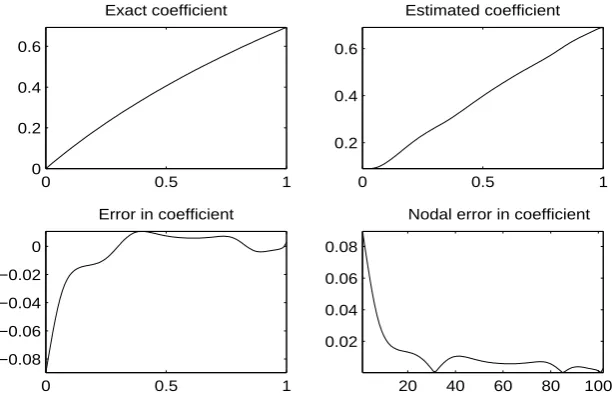
1 2 3 4 5
Exact coefficient
0 0.5 1
2 3 4
Estimated coefficient
0 0.5 1
−0.02 0 0.02 0.04
Error in coefficient
20 40 60 80 100
0.01 0.02 0.03 0.04
Nodal error in coefficient
4.3. Gradient Projection Method 29
Gradient Projection: Example 2
0 0.5 1
0 0.5 1 1.5 2
Data
0 0.5 1
0 0.5 1 1.5 2
Final simulation
0 0.5 1
−1 0 1
x 10 Error in simulated data−4
20 40 60 80 100 2
4 6 8 10 12
x 10−5 Nodal error in data
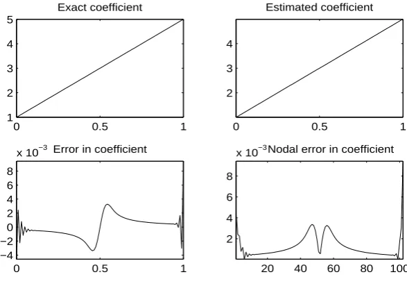
Figure 4.3: Example 2: Solution by Gradient Projection
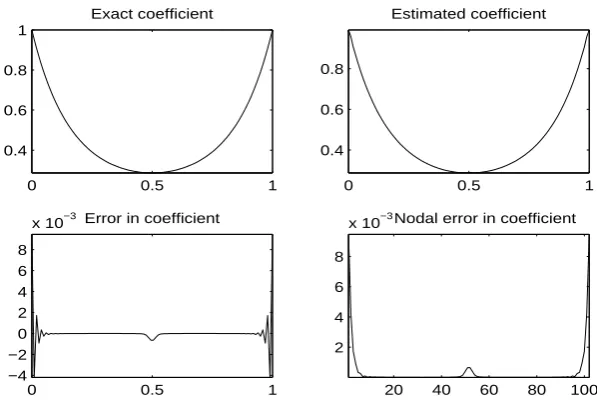
0 0.5 1
0.4 0.6 0.8 1
Exact coefficient
0 0.5 1
0.4 0.6 0.8
Estimated coefficient
0 0.5 1
−5 0 5
x 10−3Error in coefficient
20 40 60 80 100 2
4 6 8
x 10 Nodal error in coefficient−3
4.3. Gradient Projection Method 30
Gradient Projection: Example 3
0 0.5 1
−2 −1 0 1 2
Data
0 0.5 1
−1 0 1
Final simulation
0 0.5 1
−5 0 5
x 10 Error in simulated data−3
20 40 60 80 100
2 4 6
x 10−3 Nodal error in data
Figure 4.5: Example 3: Solution by Gradient Projection
0 0.5 1
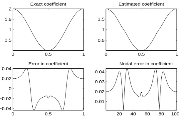
0.5 1 1.5 2
Exact coefficient
0 0.5 1
0.5 1 1.5
Estimated coefficient
0 0.5 1
−0.04 −0.02 0 0.02 0.04
Error in coefficient
20 40 60 80 100
0.01 0.02 0.03 0.04 0.05
Nodal error in coefficient
4.3. Gradient Projection Method 31
Gradient Projection: Example 4
0 0.5 1
−0.01 0 0.01 0.02 0.03
Data
0 0.5 1
−0.01 0 0.01 0.02 0.03
Final simulation
0 0.5 1
0 2 4 6
x 10 Error in simulated data−4
20 40 60 80 100 2
4 6
x 10−4 Nodal error in data
Figure 4.7: Example 4: Solution by Gradient Projection
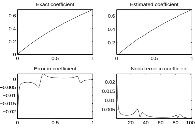
0 0.5 1
0 0.2 0.4 0.6
Exact coefficient
0 0.5 1
0.1 0.2 0.3 0.4 0.5 0.6
Estimated coefficient
0 0.5 1
−0.08 −0.06 −0.04 −0.02 0
Error in coefficient
20 40 60 80 100 0.02
0.04 0.06 0.08
Nodal error in coefficient
4.4. Scaled Gradient Projection 32
4.4
Scaled Gradient Projection
The scaled gradient projection (SGP) method has the following iterative scheme:
Ak+1 =PA˜(Ak−αkDkJ′(Ak)) (4.10)
It is common practice to take the scaling matrix Dk as the main diagonal of the Hessian of Ak with all other entries equal to zero.
Algorithm SGP Choose A0 ∈A
m, β, θ∈(0,1),0< αmin < αmax, M >0 For k= 0,1,2, ... Do the following steps:
Step 1: Chooseαk ∈[αmin, αmax] and Dk; Step 2: Projection Yk=PA˜(Ak−αDkJ′(Ak));
If Yk=Ak Stop;
Step 3: Descent direction: dk =Yk−Ak
Step 4: Setλk= 1 and fmax =max0≤j≤min(k,M−1)J(Ak−j)
Step 5: Backtracking loop: If J(Ak+λ
kdk)≤fmax+βλkJ′(Ak)Tdk Then Go to step 6;
Else
Set λk =θλk and go to step 5; EndIf
Step 6: Ak+1 =Ak+λkdk END
Here we choose αk using the Barzilai-Borwein rules:
Letrk−1 =Ak−Ak−1 and zk−1 =J′(Ak)−J′(Ak−1) with the following rules:
α(1)k = r
(k−1)T
D−k1D−k1r(k−1)
r(k−1)T
D−k1z(k−1) (4.11a)
α(2)k = r
(k−1)T
Dkz(k−1) z(k−1)T
D2
kz(k−1)
. (4.11b)
Determining αk: take a prefixed non-negative integer Mα and τ1 ∈(0,1):
If α(2)k /α(1)k ≤τk then
αk = min
(
α(2)j , j = max (1, k−Mα), ..., k
4.4. Scaled Gradient Projection 33
τk+1 = 0.9τk; Else
αk =α
(1)
4.4. Scaled Gradient Projection 34
Example 1: Scaled Gradient Projection
100 200 300 400 500 600 700 800 900
0 0.05 0.1
Gradient Norm
100 200 300 400 500 600 700 800 900
0 0.01 0.02
Function Value
100 200 300 400 500 600 700 800 900
0 2 4
x 106 Alpha
Figure 4.9: Example 1: History Output for SGP Method
0 0.5 1
0 0.1 0.2
Data
0 0.5 1
0 0.1 0.2
Final simulation
0 0.5 1
−1 0 1x 10
−4
Error in simulated data
20 40 60 80 100
0 0.5
1x 10
−4 Nodal error in data
Figure 4.10: Example 1: Solution by SGP Method
0 0.5 1
1 2 3 4 5 Exact coefficient
0 0.5 1
1 2 3 4 5 Estimated coefficient
0 0.5 1
−0.05 0 0.05
Error in coefficient
20 40 60 80 100
0.01 0.02 0.03 0.04 0.05
Nodal error in coefficient
4.4. Scaled Gradient Projection 35
Example 2: Scaled Gradient Projection
100 200 300 400 500 600 700 800 900 1000 1
2 3
Gradient Norm
100 200 300 400 500 600 700 800 900 1000 20
40
Function Value
100 200 300 400 500 600 700 800 900 1000 2000
4000 6000 8000
Alpha
Figure 4.12: Example 2: History Output for SGP
0 0.5 1
0 0.5 1 1.5 2 Data
0 0.5 1
0 0.5 1 1.5 2 Final simulation
0 0.5 1
0 5 10
x 10 Error in simulated data−5
20 40 60 80 100
2 4 6 8 10 12
x 10−5 Nodal error in data
Figure 4.13: Example 2: Solution by SGP Method
0 0.5 1
0.4 0.6 0.8 1
Exact coefficient
0 0.5 1
0.4 0.6 0.8
Estimated coefficient
0 0.5 1
−4 −2 0 2 4 6 8
x 10−3Error in coefficient
20 40 60 80 100 2
4 6 8
x 10 Nodal error in coefficient−3
4.4. Scaled Gradient Projection 36
Example 3: Scaled Gradient Projection
100 200 300 400 500 600 700 800 900 1000 1100
2 4 6 8
Gradient Norm
100 200 300 400 500 600 700 800 900 1000 1100
10 20 30 40 50 Function Value
100 200 300 400 500 600 700 800 900 1000 1100
0 2 4 6
Alpha
Figure 4.15: Example 3: History Output for SGP
0 0.5 1
−2 −1 0 1 2 Data
0 0.5 1
−1 0 1
Final simulation
0 0.5 1
−5 0 5
x 10 Error in simulated data−3
20 40 60 80 100
2 4 6
x 10−3 Nodal error in data
Figure 4.16: Example 3: Solution by SGP Method
0 0.5 1
0.5 1 1.5 2
Exact coefficient
0 0.5 1
0.5 1 1.5
Estimated coefficient
0 0.5 1
−0.02 0 0.02
Error in coefficient
20 40 60 80 100
0.01 0.02 0.03
Nodal error in coefficient
4.4. Scaled Gradient Projection 37
Example 4: Scaled Gradient Projection
50 100 150 200 250 300 350 400 450 500 550 600 5
10 15
x 10−4 Gradient Norm
50 100 150 200 250 300 350 400 450 500 550 600 1
2 3 4 5
x 10−3 Function Value
50 100 150 200 250 300 350 400 450 500 550 600 0
2 4 6
x 106 Alpha
Figure 4.18: Example 4: History Output for SGP Method
0 0.5 1
−0.01 0 0.01 0.02 0.03 Data
0 0.5 1
−0.01 0 0.01 0.02 0.03 Final simulation
0 0.5 1
0 2 4 6
x 10 Error in simulated data−4
20 40 60 80 100 1 2 3 4 5 6
x 10−4 Nodal error in data
Figure 4.19: Example 4: Solution by SGP Method
0 0.5 1
0 0.2 0.4 0.6
Exact coefficient
0 0.5 1
0.1 0.2 0.3 0.4 0.5 0.6 Estimated coefficient
0 0.5 1
−0.08 −0.06 −0.04 −0.02 0
Error in coefficient
20 40 60 80 100 0.02
0.04 0.06 0.08
Nodal error in coefficient
4.5. Extragradient Method 38
4.5
Extragradient Method
Now we explore the extra-gradient method proposed in [26] to relax the conditions on convergence for the projection method:
¯
Ak = PA˜(Ak−αJ′(Ak)) (4.12a)
Ak+1 = PA˜(Ak−αJ′( ¯Ak)), (4.12b)
where α is constant for all iterations.
In [4], convergence is proved under the conditions that ˜A is non-empty,J′ is monotone and Lipshitz (with constant L) and α ∈(0,1/L).
Convergence problems with α will be similar to the projection gradient method. When L is unknown, we may have difficulties choosing an ap-propriate α. As in the gradient projection method, if αis too small then the algorithm will converge slowly and if α is too big then it may not converge at all. Thus we will consider extragradient methods where α is an adaptive step-length.
4.5.1
Khobotov Extragradient Method
We are going to implement the adaptive steplength first introduced in [23] to remove the constraint that J′ must be Lipshitz continuous. The adaptive algorithm is of the form:
¯
Ak = PA˜(Ak−αkJ′(Ak)) (4.13a)
Ak+1 = PA˜(Ak−αkJ′( ¯Ak)). (4.13b)
Intuitively, we get better convergence whenαgets smaller between iterations, however, it is obvious that we must also control how the sequence of {αk} goes to zero.
We use the following reduction rule for αk given in [23]:
αk > β
Ak−A¯k
J′(Ak)−J′( ¯Ak), (4.14)
4.5. Extragradient Method 39
Khobotov-type Extragradient Algorithm Step 1: Chooseα, A0, and β
Step 2: ComputeJ′(Ak) Step 3: Compute ¯Ak =P
˜
A(Ak−αJ′(Ak)) Step 4: ComputeJ′( ¯Ak)
If J′( ¯Ak) = 0, STOP Step 5: If α > βJ′(AAkk)−−AJ¯′k( ¯Ak)
Then reduce αk and go to step 5; Step 6: ComputeAk+1 =P
˜
A(Ak−αJ′( ¯Ak))
Step 7: If ∥Ak+1−Ak∥< TOL Then STOP, Else go to (2)
4.5.2
Marcotte Choices for Steplength
The above algorithm requires a way to reduce αk. We are going to imple-ment the Marcotte rule [30] and its variants [37]. The original Marcotte rule incorporates the sequenceak=ak−1/2 and forcingαkto satisfy step 5 above:
αk = min
{
αk−1
2 ,
∥Ak−A¯k∥ √
2∥J′(Ak)−J′( ¯Ak)∥
}
(4.15)
Potentially we can still choose α small enough that we never reduce αk. In this case we get very slow convergence. To avoid this, we want the sequence αk to have the ability to increase if αk if αk−1 is smaller than optimal. The
first and second modified versions of Marcotte have this rule: First modified version of Marcotte
αk =αk−1+
(
β ∥A
k−1−A¯k−1∥
∥J′(Ak−1)−J′( ¯Ak−1)∥−αk−1
)
γ, (4.16)
where γ ∈(0,1).
Second modified version of Marcotte
αk = max
{
ˆ α,min
{
ξ·αk−1, β ∥
Ak−1−A¯k−1∥
∥J′(Ak−1)−J′( ¯Ak−1)∥
}}
(4.17)
4.5. Extragradient Method 40
Example 1: Marcotte methods (all three versions)
0 5000 10000
0 1 2 3 4
x 10−4 Gradient Norm
0 5000 10000
2 4 6 8 10x 10
−4 Function Value
2000 4000 6000 8000 10000 0
50 100
Alpha
2000 4000 6000 8000 10000 0.01
0.02 0.03 0.04 0.05
Norm(xk+1−xk)
Figure 4.21: Example 1: History Output for Marcotte Method
0 0.5 1
0 0.05 0.1 0.15 0.2 Data
0 0.5 1
0 0.05 0.1 0.15 0.2 Final simulation
0 0.5 1
−5 0 5
x 10 Error in simulated data−5
20 40 60 80 100
2 4 6 8
x 10−5 Nodal error in data
Figure 4.22: Example 1: Solution by Marcotte Methods
0 0.5 1
1 2 3 4 5 Exact coefficient
0 0.5 1
2 3 4
Estimated coefficient
0 0.5 1
−0.02 0 0.02 0.04
Error in coefficient
20 40 60 80 100
0.01 0.02 0.03 0.04
Nodal error in coefficient
4.5. Extragradient Method 41
Example 2: Marcotte Methods (all three versions)
200 400 600 800 1000
0 0.01 0.02
Gradient Norm
200 400 600 800 1000
0 0.01 0.02
Function Value
200 400 600 800 1000
0.8 0.9 1 1.1
Alpha
200 400 600 800 1000
0 0.01 0.02
Norm(xk+1−xk)
Figure 4.24: Example 2: History Output for Marcotte SMV Method
0 0.5 1
0 1 2
Data
0 0.5 1
0 0.5 1 1.5 2 Final simulation
0 0.5 1
0 1 2
x 10 Error in simulated data−4
20 40 60 80 100 0.5
1 1.5 2
x 10−4 Nodal error in data
Figure 4.25: Example 2: Solution by Marcotte Methods
0 0.5 1
0.4 0.6 0.8 1
Exact coefficient
0 0.5 1
0.4 0.6 0.8
Estimated coefficient
0 0.5 1
0 5 10
x 10−3Error in coefficient
20 40 60 80 100
2 4 6 8 10 12
x 10 Nodal error in coefficient−3
4.5. Extragradient Method 42
Example 3: Marcotte Method (similar to the first variant)
2000 4000 6000 8000 10000 0 0.05 0.1 0.15 0.2 Gradient Norm
2000 4000 6000 8000 10000 0.1
0.15 0.2 0.25
Function Value
2000 4000 6000 8000 10000 0.05
0.1 0.15
Alpha
2000 4000 6000 8000 10000 0
5 10x 10
−3 Norm(xk+1−xk)
Figure 4.27: Example 3: History Output for Marcotte Method
0 0.5 1
−2 −1 0 1 2 Data
0 0.5 1
−2 −1 0 1 2 Final simulation
0 0.5 1
−5 0 5
x 10 Error in simulated data−3
20 40 60 80 100 1
2 3 4 5
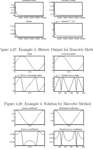
[image:52.595.150.452.176.660.2]x 10−3 Nodal error in data
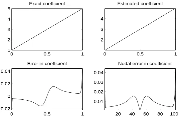
Figure 4.28: Example 3: Solution by Marcotte Method
0 0.5 1
0.5 1 1.5 2
Exact coefficient
0 0.5 1
0.5 1 1.5
Estimated coefficient
0 0.5 1
−0.02 0 0.02
Error in coefficient
20 40 60 80 100
0.01 0.02 0.03
Nodal error in coefficient
4.5. Extragradient Method 43
Example 3: Second Marcotte Method
2000 4000 6000 8000 10000 0 0.05 0.1 0.15 0.2 Gradient Norm
2000 4000 6000 8000 10000 0 0.05 0.1 0.15 0.2 Function Value
2000 4000 6000 8000 10000 0.005 0.01 0.015 0.02 0.025 Alpha
2000 4000 6000 8000 10000 0
0.5 1x 10
−3 Norm(xk+1−xk)
Figure 4.30: Example 3: History Output for Marcotte SMV Method
0 0.5 1
−1 0 1
Data
0 0.5 1
−1 0 1
Final simulation
0 0.5 1
−4 −2 0 2 4
x 10 Error in simulated data−4
5 10 15 20
1 2 3 4
x 10−4 Nodal error in data
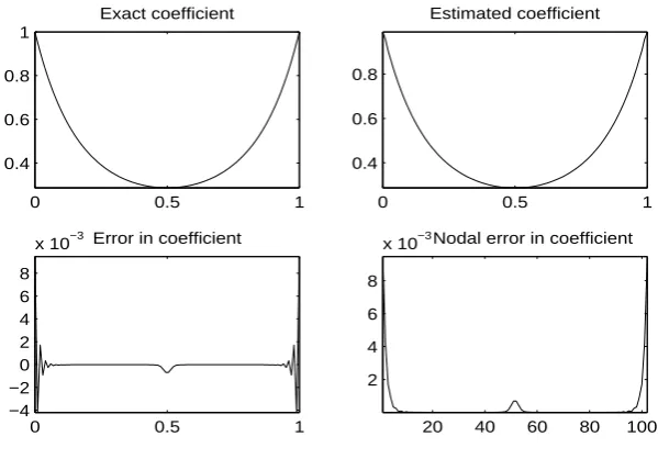
Figure 4.31: Example 3: Solution by Marcotte SMV Method
0 0.5 1
0.5 1 1.5 2
Exact coefficient
0 0.5 1
0.5 1 1.5
Estimated coefficient
0 0.5 1
−5 0 5 10 15x 10
−3Error in coefficient
5 10 15 20
5 10 15
x 10 Nodal error in coefficient−3
4.5. Extragradient Method 44
Example 4: Marcotte Method (similar first variant)
2000 4000 6000 8000 10000 0
5 10x 10
−4 Gradient Norm
2000 4000 6000 8000 10000 0
1 2
x 10−4 Function Value
2000 4000 6000 8000 10000 20
40 60 80
Alpha
2000 4000 6000 8000 10000 0
0.01 0.02
Norm(xk+1−xk)
Figure 4.33: Example 4: History Output for Marcotte FMV Method
0 0.5 1
−0.01 0 0.01 0.02 0.03 Data
0 0.5 1
−0.01 0 0.01 0.02 0.03 Final simulation
0 0.5 1
0 2 4 6
x 10 Error in simulated data−4
20 40 60 80 100 1 2 3 4 5 6
x 10−4 Nodal error in data
Figure 4.34: Example 4: Solution by Marcotte Method
0 0.5 1
0 0.2 0.4 0.6
Exact coefficient
0 0.5 1
0.1 0.2 0.3 0.4 0.5 0.6 Estimated coefficient
0 0.5 1
−0.08 −0.06 −0.04 −0.02 0
Error in coefficient
20 40 60 80 100 0.02
0.04 0.06 0.08
Nodal error in coefficient
4.5. Extragradient Method 45
Example 4: Second Marcotte Method
2000 4000 6000 8000 10000 0
5 10x 10
−5 Gradient Norm
2000 4000 6000 8000 10000 0
5 10
x 10−4 Function Value
2000 4000 6000 8000 10000 20
40 60 80
Alpha
2000 4000 6000 8000 10000 0
0.01 0.02
Norm(xk+1−xk)
Figure 4.36: Example 4: History Output for Marcotte SMV Method
0 0.5 1
−0.01 0 0.01 0.02 0.03 Data
0 0.5 1
−0.01 0 0.01 0.02 0.03 Final simulation
0 0.5 1
0 1 2 3 4
x 10 Error in simulated data−4
20 40 60 80 100 1
2 3 4
x 10−4 Nodal error in data
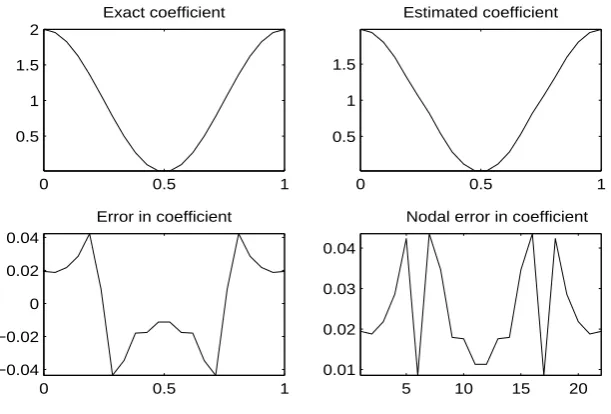
Figure 4.37: Example 4: Solution by Marcotte SMV Method
0 0.5 1
0 0.2 0.4 0.6
Exact coefficient
0 0.5 1
0.1 0.2 0.3 0.4 0.5 0.6 Estimated coefficient
0 0.5 1
−0.06 −0.04 −0.02 0
Error in coefficient
20 40 60 80 100 0.02
0.04 0.06
Nodal error in coefficient
4.6. Scaled Extragradient Method 46
4.6
Scaled Extragradient Method
Now we consider a projection-contraction type extragradient method pre-sented by Solodov and Tseng in [34]. It involves a scaling matrix to accelerate convergence.
¯
Ak = PA˜(Ak−αkJ′(Ak)) (4.18)
Ak+1 = Ak−γM−1(Tα(Ak)−Tα(PA˜( ¯Ak)) (4.19)
where γ ∈ R+ and T
α = (I−αJ′); here, I is the identity matrix, and α is chosen such that Tα is strongly monotone.
Additional discussion of the scaling matrix is given in [37], however, in both [37] and [34], test problems take M equal to the identity matrix.
Solodov-Tseng Method Step 1: Choose A0, α
−1, θ ∈(0,2), ρ, β∈(0,1), M ∈Rm×m
Step 2: ¯A0 = 0, k = 0, rx =ones(m,1) Step 3: if ∥rx∥< TOL then STOP
else α=αk−1, f lag= 0;
Step 4: if J′(Ak) = 0 then STOP
Step 5: While α(Ak−A¯k)T(J′(Ak)−J′( ¯Ak))>(1−ρ)∥Ak−A¯k∥2 or f lag = 0 Iff lag ̸= 0 Then α=αk−1β endif
update ¯Ak =PA˜(Ak−αJ′(Ak)), computeJ′( ¯Ak)
f lag=f lag+ 1; endwhile
Step 6: update αk =α;
Step 7: compute γ =θρ∥Ak−A¯k∥2/∥M1/2(Ak−A¯k−α
kJ′(Ak) +αkJ′( ¯Ak))∥2; Step 8: compute Ak+1 =Ak−γM−1(Ak−A¯k−α
kJ′(Ak) +αkJ′( ¯Ak)) Step 9: rx=Ak+1−Ak, k=k+ 1 go to step (3)
The Solodov-Tseng method suggests a more general form for the advanced extragradient methods:
¯
Ak = PA˜(Ak−αkJ′(αk)) (4.20a)
Ak+1 = PA˜(Ak−ηkJ′( ¯Ak)), (4.20b)
4.6. Scaled Extragradient Method 47
Example 1: Solodov-Tseng Method
0 0.5 1
0 0.05 0.1 0.15 0.2
Data
0 0.5 1
0 0.05 0.1 0.15 0.2
Final simulation
0 0.5 1
−5 0 5
x 10 Error in simulated data−5
20 40 60 80 100
2 4 6 8
[image:57.595.153.457.173.377.2]x 10−5 Nodal error in data
Figure 4.39: Example 1: Solution by Solodov-Tseng Method
0 0.5 1
1 2 3 4 5
Exact coefficient
0 0.5 1
2 3 4
Estimated coefficient
0 0.5 1
−0.02 0 0.02 0.04
Error in coefficient
20 40 60 80 100
0.01 0.02 0.03 0.04
Nodal error in coefficient
[image:57.595.152.457.419.627.2]4.6. Scaled Extragradient Method 48
Example 2: Solodov-Tseng method
0 0.5 1
0 0.5 1 1.5 2
Data
0 0.5 1
0 0.5 1 1.5 2
Final simulation
0 0.5 1
0 5 10
x 10 Error in simulated data−5
20 40 60 80 100 2
4 6 8 10 12
[image:58.595.157.457.173.376.2]x 10−5 Nodal error in data
Figure 4.41: Example 2: Solution by Solodov-Tseng Method
0 0.5 1
0.4 0.6 0.8 1
Exact coefficient
0 0.5 1
0.4 0.6 0.8
Estimated coefficient
0 0.5 1
−4 −2 0 2 4 6 8
x 10−3Error in coefficient
20 40 60 80 100
2 4 6 8
x 10 Nodal error in coefficient−3
[image:58.595.156.456.419.628.2]