Algorithms and implementation of functional dependency discovery in XML : a thesis presented in partial fulfilment of the requirements for the degree of Master of Information Sciences in Information Systems at Massey University

ALGORITHMS AND IMPLEMENTATION

OF FUNCTIONAL DEPENDENCY

DISCOVERY IN XML

A thesis presented in partial fulfilment

of

the requirements for

the degree

of

MASTER OF INFORMATION SCIENCES

IN

INFORMATION SYSTEMS

at

Massey University, Palmerston North, New Zealand

Acknowledgement

I wish to take this opportunity to give my sincere thanks to Associate Professor, Dr. Sven Hartmann for his kind and enlightening guidance and constructive suggestions throughout this research and valuable recommendations on improvement of the thesis. It has been my pleasure to meet those wonderful people at the University and I have developed a solid friendship with many of them; without their support in varied forms, it would have been an arduous year for me. Particularly, I am thankful to Madre Chrystall for her inspiring encouragement, valuable technical advice on MySQL and kind proofreading. I also benefited from discussions with Thu Trinh who shared with me her knowledge on Latex. Furthermore, the Massey Masterate Scholarship which I was awarded in 2005 academic year has made my life financially manageable.

Finally, I owe my entire life and all my success to my parents for their incomparable enormous love; they are appreciated, respected and treasured by me forever and a day. My heart is always warmed also by the fondness from my aunt and my sister. They light up my life and are my everything.

Contents

1 Introduction

1.1 Background

1.2 Motivations

1.3 Related Work

1.3.1 Hypothesis Research

1.3.2 Schema Derivation Algorithms . 1.3.3 Schema Tree Inference Algorithms .

6

6

6

9

9

. . . . . . . . . 10

11 1.3.4 XML-RDB Mapping . . . . . . . . . . . . . . . 12

1.4 Our Contribution . . . . . . . . . . . . . . . . . . . . . . . . . . 14

1.5 Thesis Outline . . . . . . . . . . . . . . . . . . . . . . . . . . . . . 14

2 XML Essentials 2.1 XML Basics . 2. 2 XML Schema Schemes 15 . . . . . . . . . . . . . . . . . . . . . . . 15

. . . . . . . . 16

2.2.1 The DTD (Document Type Definition) Family . . . . . . . . . 16

2.2.2 The W3C XSD (XML Schema Definition) Family . . . . . . . . . . 16

CONTENTS

2.2.4 The DataGuide Family . .

2.3 Functional Dependencies in XML

3 XML Schema Extraction

3.1 Element Relationship Model for XML (ER-XML)

3.2 ER-XML Extraction .. . .. . . .. . .. .

3

17

18

19

19

. . . . . 23

3.2.1 Depth-First Search (DFS) vs. Breadth-First Search (BFS) . . . . . 23

3.2.2 ER-XML Extraction (EXE) Algorithm . . . . . . . . . . . . . . 25

4 XML-Relation Data Transformation 29 4.1 Preliminary Definitions . . . . . . . . . . . . . . . . . . . . . . . . . 29

4.1.1 Rooted Tree and XML Tree . . . . . . . . . . . . . . . . . . . . 29

4.1. 2 XML Schema Tree . . . . . . . . . . . . . . . . . . . . . . . . 30

4.1.3 XML Schema Tree Features 30 4.1.4 Mappings between XML Trees . . . . . . . . . . . . . . . . . . 31

4.1.5 XML Data Tree . . . . . . . . . . . . . . . . . 33

4.1.6 Functional Dependencies for XML . . . . . . . . . . . . . . . . 33

4.1.7 Schema Vertex Table . . . . . . . . . . . . . . . . . . . . . . . . . . 35

4.2 Transformation Methodology . . . . . . . . . . . . . . . . . . . . . . . . . . 36

4.3 The Algorithm SVT-Trans . . . . . . . . . . . . . . . . . . . . . . . . 39

4.3.1 SVT-Trans Overview . . . . . . . . . . . . . . . . . . . 39

4.3.2 Handling NULL Values . . . . . . . . . . . . . . . . . . . . . . 42

CONTENTS

5.1

5.2

5.3

System Overview . .

5.1.1

5.1.2

Functionality

System Architecture

Functional Dependency Inference Algorithms .

5.2.1

5.2.2

5.2.3

The Naive Algorithm . . . .

The Enhanced Algorithm Using Transversals .

The Enhanced Algorithm FastFDs

Implementation Considerations . . . .

5.3.1

5.3.2

5.3.3

5.3.4

Programming language - Java

Data Definition and Manipulation Language - MySQL .

XML Parser - DOM.

Data Structure . . . .

6 Case Study

6.1 Walking Through XFD-Miner

6.2 Performance Testing . . . . .

7 Conclusion and Future Work

7.1 Conclusion ..

7.2 Future Work .

A XFD-Miner Guide

A. l Environment Configuration

A.2 Run XFD-Miner . . . .

CONTENTS

A. 2 .1 Installed Directory Tree

A.2.2 Execute XFD-Miner

A.3 Miscellaneous . . . .

5

. . . . . . 69

.. . . .. . . 70

. . . . . . . . . . . . . . . . 71

B Sample XML document: warehouse.xml 72

Chapter 1

Introduction

1.1

Background

Following the advent of the web, there has been a great demand for data interchange between applications using internet infrastructure. XML (eXtensible Markup Language) provides a structured representation of data empowered by broad adoption and easy

deployment. As a subset of SGML (Standard Generalized MarkupLanguage), XML has been standardized by the World Wide Web Consortium (W3C) [Bray et al., 2004]. XML is becoming the prevalent data exchange format on the World Wide Web and increasingly significant in storing semi-structured data. After its initial release in 1996, it has evolved

and been applied extensively in all fields where the exchange of structured documents in

electronic form is required.

As with the growing popularity of XML, the issue of functional dependency in XML has

recently received well deserved attention. The driving force for the study of dependencies in XML is it is as crucial to XML schema design, as to relational database(RDB) design

[Abiteboul et al., 1995].

1.2 Motivations

As semi-structured data has become prevalent with the growth of the Internet and other

on-line information repositories, many organisational databases are presented on the web as semi-structured data. Designing a 'good' semi-structured database is increasingly

1.2. MOTIVATIONS 7

cial to sustain data integrity and prevent data redundancy, inconsistency and updating anomalies. Redundant information caused by functional dependencies in XML may give rise to such problems. Therefore, identifying XML functional dependencies and thus achieving normalisation becomes vital in good XML design.

Often in design practice, we are facing a task of finding all possible functional dependencies satisfied by a given XML document, which may imply business rules. Thus emerges a new research direction: the XML dependency discovery problem, on which however, little investigation has been conducted so far though a breakthrough would be of prominent value in practice.

XML schema plays a substantial role in discovering functional dependencies of XML data, since they are defined on top of schematic information, as with relational databases.

In addition, it is well-known that XML schema information specifies the internal structure of an XML document, which realises the promise of XML as the universal data represen-tation format enabling free electronic data interchange (EDI) and integration of disparate data sources. It is also critical in the efficient storage of XML data as well as formulation, optimisation and query processing [Garofalakis et al., 2000]. Unfortunately, in practice many XML documents are not associated with schema definitions, giving rise to the task of inferring the schematic information from XML documents.

Our preliminary feasibility studies on XML dependency discovery have suggested the 'divide-and-conquer' strategy, leading to the following problem decomposition:

1. XML Schema Extraction

This is determined by the fact explained previously that XML schema information is essential but absent in most cases. Certain generalisation of input data is often required in schema extraction; ideally the extracted schema should, on one hand, tightly represent the data, and be concise and compact on the other hand. As the two requirements essentially contradict each other, finding an optimal tradeoff is a difficult and challenging task [Chidlovskii, 2001].

2. XML-Relation Data Transformation

CHAPTER 1. INTRODUCTION 8

format with the help of its schema. The inspiration for such a transformation

comes from appreciation of over 20 years of work invested in relational database technology. Relational functional dependencies have been well explored and some

inference algorithms with satisfactory performance are already in existence, which we can leverage to assist in discovering functional dependencies in XML. There have been some research endeavours on mapping XML documents to relational tables, as

further illustrated in the section 'Related Work'.

3. Relational FD Inference

The final step is to apply some well-developed relational functional dependency inference algorithms to the data in relational format after the transformation to

achieve our ultimate goal.

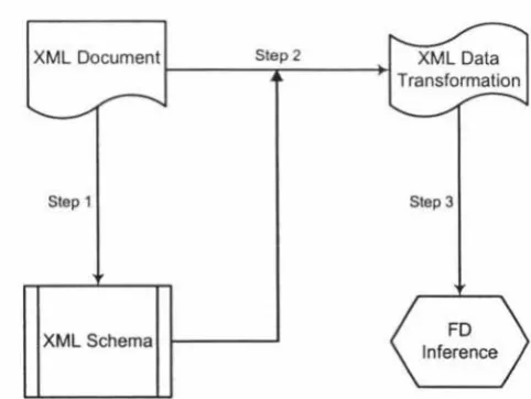
Figure 1.1 shows the entire work flow:

XML Document Step2

I , .

-Step 1

XML Schema

XML Data

Transformation

Step 3

FD

Inference

1.3. RELATED WORK 9

1.3 Related Work

1.3.1

Hypothesis Research

The inference of structure out of semi-structured data has been long-standing in the XML research area [Sakakibara, 1997]. Some approaches investigated possible solutions derived from theoretical grammatical inference and were very powerful at the conceptual

level. [Ahonen, 1996] presented a technique based on machine learning, with the help

of finite-state automata describing the given instances completely. These automata were

modified by considering certain context conditions, corresponding to generalisation of the underlying language, which were then converted into regular expressions to construct

the grammar. Although traditional grammatical inference methods for DTD generation stated in [Ahonen, 1996] are theoretically appealing (as they guarantee to infer languages

falling within certain language classes), it is not clear whether the structure within the

limited context is valid in practice, i.e., its theoretical appeal may not necessarily translate

into practical applicability.

[Young-Lai, 1996] discussed a grammatical inference method generating stochastic finite

automata using an adapted stochastic method and attempted to improve it by isolating low frequency data components and allowing adjustment at the generalisation level. This

approach was derived from more recent work in grammatical inference, with the base

algorithm known as Alergia [Carrasco and Oncina, 1994]. As with the methods of Ahonen, Alergia has strong theoretical significance. Again, though, our interest lies in practical performance. Moreover, none of them even touched the problem of how to present schema information with high understandability to the user.

[Garofalakis et al., 2000] proposed XTRACT, a specialized DTD induction system con-sisting of a generation module, a factoring module and an MDL1 (Minimum Description Length) module. XTRACT employed generalisation and factorisation of regular expres-sions, to derive a pool of candidate DTDs, and then used the MDL principle as the basis to make a final selection. Still, XTRACT requires human intervention and judgement in making a choice out of all candidates.

CHAPTER 1. INTRODUCTION 10

1.3.2

Schema Derivation Algorithms

Some research focusing on XML practice has also been going on, mainly centring on DTD and schema tree extraction. [Chen, 1991] talked about generation of 'de-facto grammar', which simply aggregated structures of all XML instances to be the DTD. The de-facto grammar is obviously far too simple and limited.

[Chidlovskii, 2002] modelled the XML schema as extended context-free grammars and developed an extraction algorithm inspired by methods of grammatical inference. The algorithm was also said to cope with the schema determinism requirement imposed by XML DTDs and XML Schema languages. He defined (range) Extended Context Free Grammar (ECFG) as a 5-tuple G

=

like t B t', briefly t: B, where t, t' ET and BE NU D. The extraction algorithm firstly generalized ECFG from XML content, which was then transformed to an XML schema definition. Details of the algorithm are shown in Figure 1.2:

0. Represent XML documents as set I of structured examples.

1. Induce an extended context-free grammar G from J:

1.1 Create the initial set of nonterminals N:

1.2 Merge nonterminals in N with the similar content and context;

1.3 Determine tight datatypes for terminals in G;

1.4 Generalize contents in nonterminals into range REs.

2. Transform the result ECFG G into an XML Schema definition S.

Figure 1.2: ECFG Extraction Algorithm (Adapted from [Chidlovskii 2002, p. 292])

In addition to work concerned with the problem of DTD inference, there have also been

many papers published on related topics. Most notable amongst these is work within the

Lore semistructured database project to infer DataGuides [Goldman and Widom, 1997].

This included the MakeDataGuide algorithm to construct a strong DataGuide over a

source database as shown in Figure 1.3 - A DataGuide is strong iff it shares exactly

1.3. RELATED WORK 11

any technical aspects, such as data structure, i.e., how the schematic information can be actually stored and utilised.

/ / Input: o, the aid of the root of a source database

/ / Effect: dg is set to be the root of a strong DataGuide for o

targetHash = global empty hash table, to map source target sets to DataGuide objects

dg = global aid

MakeDataGuide( o) {

}

dg = NewObject()

targetHash.Insert( o, dg)

RecursiveMake( o, dg)

RecursiveMake(tl, dl) {

}

p = set of <label, oid> children pairs of each object in t1

foreach ( unique label l in p) { t2 = set of oids paired with l in p

d2 = targetHa.sh.Lookup(t2)

if (d2 != nil) {

add an edge from dl to d2 with label l

} else {

}

}

d2 = NewObject()

targetHa.sh.Insert(t2, d2)

add an edge from dl to d2 with label l RecursiveMake( t2, d2)

Figure 1.3: Algorithm MakeDataGuide (Adapted from [Goldman et al. 1997 , Figure 4,

p. 8])

1.3.3

Schema Tree Inference Algorithms

The subject of schema tree and related issues, such as tree extraction, are not recent in

research area. A labelled tree specifying nesting relationships between labelled vertices was referred to as XML schema tree elements [Cruz et al., 2004]. A schema tree was also

CHAPTER 1. INTRODUCTION 12

sequence (','), repetition ('*'), union ('I'),

<

>

<

(

[Chen et al., 2002] stated a schema tree generation algorithm as displayed below:

ALGORITHM 3: Generate schema tree

INPUT: Node N of the tree T' constructed at Step 7 in Algorithm 1 OUTPUT: Schema tree

Step 1: if N is a leaf node then return; Step 2: for all child node C of node N do

Step 3: if name of edge E which connect C and N existed at the same level then{ Step 4: find node C'and corresponding edge E'holding same name with E, which

connects C' and N;

Step 5: all subtrees of C is moved to be subtrees of C'; Step 6: delete node C and edge E;}

Step 7: for all child node C of node N do

Step 8: recursively applying algorithm 3 from node C;

Fig.9: Generate schema tree algorithm

Figure 1.4: Schema Tree Generation (Adapted from [Chen et al. 2002 , Figure 9, p.84])

There are at least three deficits in this algorithm: firstly, it only considers, compares and

processes identical elements appearing at the same level (in Step 3), exclusive of the

sce-nario with one element occurring at different levels. Secondly, it just simply aggregates subtrees of all occurrences of an element (node) (in Step 5), which will merely give a

document tree at most, instead of a schema tree as supposed. Third, structural informa-tion captured is rather poor; only a collection of possible sub-element names, without any

knowledge of element order, whether they are optional, compulsory, or iterating.

1.3.4 XML-RDB Mapping

Researchers have already shown their interest in transforming data in XML format into

relational database. [Christophides et al., 1994] proposed a one-to-one mapping from each element declaration in the DTD to a relation. It is apparently a simple way of generating

corresponding relational schema but likely leads to excessive fragmentation.

[Shanmugasundaram et al., 1999] suggested analyse a DTD and automatically convert it

to a set of relational schemata. To do this, the original DTD should be firstly simplified

1.3. RELATED WORK 13

• Basic approach Generate a DTD graph after grouping or flattening element frequency specifications and the respective element graph on which the relational schemata are decided;

• Shared approach Create a separate relation for each element node represented by multiple relations in the basic approach, and share this relation; or

• Hybrid approach element processing.

Same as the shared approach except for some variance in

Their work will also result in excessive fragmentation of DTDs, causing unnecessary data scatter, which incurs unaffordable cost from joins when multiple relations need to be accessed.

A new inlining algorithm was put forward by [Lu et al., 2003], featuring modeling XML attributes as XML elements since they can be treated as elements without further nesting structure. It comprises similar steps as the others: Create a DTD graph after DTD simplification and inline as many descendant elements as possible to an XML element to eliminate redundancy caused by shared elements in the generated schema, which is to be eventually generated based on the inlined DTD graph. Such an inlining algorithm can relatively reduce redundancy in comparison to the shared approach introduced previously, though data scatter is still present.

[Yan and Fu, 2001] described construction of schema prototype trees representing the structure of a simplified DTD and subsequent generation of relational schema proto-types. They also briefly mentioned functional dependency and candidate key detection and relational schema prototype normalisation techniques.

CHAPTER 1. INTRODUCTION 14

1.4

Our Contribution

In our research, we delved into both schema extraction and the XML-Relation data trans-formation problem. A novel data representation model, ER-XML (Element Relationship model for XML) was devised, utilising an implementation-focused algorithm capable of being directly applied to XML practice. ER-XML can also help to extract and identify cardinality constraints. The data structure invented was properly designed to facilitate graphical representation generation as well as compatibility validation. As for

XML-Relation transformation, we have developed an entire set of algorithms, SVT-Trans with the help of ER-XML and the concept of 'Almost Copy' in XML tree, which retrieves semantic data from an original XML document and places them into a relational for-mat using recursion computation. The output of SVT-Trans can be directly exploited by relational functional dependency discovery algorithms. A prototype system was also successfully implemented and a case study was provided which demonstrated correctness and soundness of our work.

1.5

Thesis Outline

Chapter

2

XML Essentials

This chapter provides background knowledge on XML standards and related technology. We start with an overview of XML, then its assorted schema languages and finally func-tional dependency issues in XML.

2.1

XML Basics

As a metalanguage used to define new markup languages, XML was developed by the W3C1 (World Wide Web Consortium). It has been well acknowledged as a standard for data representation and exchange on the Internet. Unlike HTML, which was designed to display data, XML is intended to describe structured data [Sun Microsystems Inc., 2002]; it allows designers to create their own customised tags, enabling the definition, transmission, validation and interpretation of data between applications and between organisations[Gaskin, 2000]. Besides, XML will enable a new generation of web-based data viewing and manipulation applications.

XML documents are composed of content and markup by way of nested pairwise start-and end-tags. There are some kinds of markup that can occur in an XML document, for instance elements, attributes, entity references and document type declarations, with the first two particularly pertinent to our work2.

A decent XML document must be well-formed. The well-formedness of an XML

doc-1 _{It first became a W3C Recommendation on 10 February 1998.}

2_{Relevant fundamental knowledge on XML is assumed for the reader and thus not reiterated here.}

CHAPTER 2. XML ESSENTIALS 16

ument is ensured by enforcing proper nesting as for its logical and physical structure [Bray et al., 2004]. Those grammatical features need to be captured as schema and will be used in the validation process of an arbitrary XML document.

2.2

XML Schema Schemes

At present, several XML schema schemes are widely used, including DTD, XML schema, Relax NG, DataGuide and so forth. It is worthy of note that the first three are prescrip-tive schema clearly defining and imposing legitimate components and structure, whereas DataGuide serves as a descriptive schema only depicting and inferring structural infor-mation from an existing XML document.

2.2.1

The DTD (Document Type Definition) Family

Inherited from SGML, DTD is the most widely deployed means of defining an XML schema. Its purpose is to specify document structure and legal building blocks, such as

elements and attributes of an XML document (Bray et al. 2000). The W3C Recommenda-tion on XML defines a DTD as containing or pointing to markup declarations that provide a grammar for a class of documents, such as entity declaration, element type declaration and attribute-list declaration. A DTD, to the author, is indeed a formal prescription in XML declaration syntax of a desired document, which sets out what names are to be used for the different types of elements and associated attributes, where they may occur, and how they all fit together.

2.2.2

The W3C XSD (XML Schema Definition) Family

W3C has developed XSD to provide an alternative to XML DTD that supports names-paces, facilitates the design of open and extensible vocabularies, and meets the require-ment of data-oriented applications for a richer datatyping system. It does so by borrowing

2.2. XML SCHEMA SCHEMES 17

recommendation which describes the validation process more than the modelling features. W3C XSD is a strongly typed schema language that eliminates any non-deterministic design from the described markup to ensure that there is no ambiguity in the

determi-nation of the datatypes and that the validation can be made by a finite state machine [Fallside and Walmsley, 2004].

2.2.3 Th

e

RELAX NG F

am

il

y

RELAX NG is a schema language rooted in finite tree automata (FTA) that can be used to validate an XML document against a particular schema. It is formed by the unification of TREX [Clark, 2001] with RELAX [Murata, 2001], adopting XML for writing schemas. Its syntax appears similar to a description of the instance document in ordinary English and simpler than W3C XML Schema. Some constraints, especially those on the fringe of non-deterministic models and combinations in document structure can be expressed by RELAX NG but not W3C XML Schema. RELAX NG arranges markup declarations as XML syntax itself, such as <element name="">, <attribute name="">. Additional integrity constraints are also expressed in pairwise tags, <zeroOrMore>, <oneOrMore>

and <optional> for instance, compared to'*',

'+'

2.2.

4

Th

e

DataGuid

e

Fa

mily

DataGuide was released as a partial outcome of the Lore (Lightweight Object Repository) project at Stanford University in the late 1990s, which extends the theoretical foundation of Representative Objects (ROs) [Nestorov et al., 1997] and the Object Exchange Model (OEM) [Papakonstantinou et al., 1995]. It is a concept of dynamically generated struc-tural summaries of graph-structured databases and an object data model, respectively [Goldman and Widom, 1997]. Goldman et al. [1997, p. 5] defined that 'DataGuide for an OEM source object s is an OEM object d such that every label path of s has exactly

CHAPTER 2. XML ESSENTIALS 18

schema. Therefore DataGuide, as a descriptive schema, reflects data and its changes,

instead of forcing data to adhere to a predefined schema as relational and object-oriented databases. In fact, DataGuide should be categorised under XML schema graph, which was established as 'an XML graph where no two successors of the same vertex have the same name and the same kind' [Hartmann et al., 2003]. Goldman et al. also proposed a path index, strong DataGuide, with the building algorithm analogous to conversion from

a non-deterministic finite automaton (NFA) to a deterministic finite automaton (DFA). [Milo and Suciu, 1999] believed that it was just a simple labelled path and unsuitable for complex path queries with regular expressions. In addition, there is certainly a substantial overhead for extracting and maintaining DataGuide repositories of unmanageably large

size.

2.3

Functional Dependencies in XML

Normalisation as a design technique has long been widely used as a guide in designing relational databases. It is essentially to create a set of relational tables that are free of redundant data and that can be consistently and correctly modified through a two

Chapter 3

XML Schema Extraction

In this chapter we elaborate the ER-XML model which has been devised to capture

schematic information of an XML document, its graphical representation, and the

ER-XML Extraction (EXE) algorithm detailing the specific steps in building up an ER-XML

model out of an XML document.

3.1

Element Relationship Model for XML

(ER-XML)

DTD declaration in XML documents and no such DTD association in existence drives

XML schema extraction, deriving schema information from an XML data source based on

only the XML data source. The rationale is that in semistructured data, the information

normally associated with a schema is contained within the data, so-called "self-describing"

[Buneman, 1997], on which we have contrived a comprehensive data representation model

ER-XML.

Without loss of generality, the following assumptions are taken in our research:

1. Usage of name space is not of our interest.

It is not our everyday encounter and support for name space can always be

incor-porated afterwards.

2. 'ID', 'IDREF' and 'IDREFS' are also beyond our consideration.

CHAPTER 3. XML SCHEMA EXTRACTION 20

ID, IDREF, and IDREFS are analogous to PK/FK (primary key/foreign key) rela-tionships in relational databases, with few differences.

ER-XML captures essential structural information out of an XML instance, still with

complementary desirable features, such as simplicity, high usability and applicability.

Nevertheless, it has only three basic concepts: element, relationship and cardinality.

1. Element

An element corresponds to a vertex in an XML schema tree. There is some similarity

between element and entity type in traditional data modelling. An entity type has

a name and is characterized by the set of attributes that belongs to that entity,

whereas an element in ER-XML is described only by its name (tag name) in that

semistructured data is normally less structured, i.e. the set of sub-elements and attributes associated with each instance of a certain element varies. As a result, an element is identified by its name and represented as a labelled node in ER-XML.

There exist two types of element:

• An element serves as a base element if there is at least one occurrence of it in the XML source.

• An element serves as a non-base element if at least one occurrence of it in the XML source appears as a descendent of a base element.

The categorisation as 'base' or 'non-base', only refers to the role that an element can take. Obviously, it does not exclude that an element can be both, which is often the case, as in Figure 3.1 'State' should appear in the ER-XML model twice, with the role of 'non-base' and 'base', respectively:

The dual-role property of an element is indeed determined by the fact that an internal node in an XML tree structure can be a 'parent' node and a 'child' node at the same time1_{. Each base element has a non-base element set, which turns out to}

be an empty set for a leaf node.

2. Relationship

3.1. ELEMENT RELATIONSHIP MODEL FOR XML (ER-XML)

State serves both as a

~ - - - ! child (to Country) and

as a parent (to City)

Figure 3.1: Base and Non-Base Role Example

21

Due to the observation that an element may well take two roles, XML schema tree

structure can be constructed by putting together all 'parent-child' element pairs.

Therefore in ER-XML we concentrate on the 'parent-child' relationship of elements,

representing 'parent-child' in an XML schema tree. Such a relationship in an

ER-XML diagram is represented by an arc connecting a parent and its child with an

arrowhead pointing to the latter.

3. Cardinality

As part of the work on establishing requirements for W3C XML Schema, the

Work-ing Group are seeking information about usage patterns of numerical occurrence

con-straints in content models, i.e. 'minOccurs' or 'maxOccurs' with a more specific

nu-meric value other than 0, 1, or wildcards on elements [Fallside and Walmsley, 2004].

Also for that reason, it becomes essential to extract such occurrence information

from a source document.

Capability of recording element cardinality details is another facility of ER-XML.

It is well known that occurrences of an element in an XML document can be

stip-ulated in its DTD_ using frequency constraints, such as '?'(optional), '*'(optional

and repeatable). Unfortunately an XML document itself in the absence of DTD is

not fully expressive in terms of element cardinality and optionality. For instance, a

single presence of an element in an XML file indicates it is either a mandatory or an

optional occurrence since a particular XML instance does not exhaust all legitimate

CHAPTER 3. XML SCHEMA EXTRACTION 22

the minimal and maximum number of occurrences of every element, despite many

possible cases of it. In an ER-XML diagram, cardinality information of each element

is displayed next to the corresponding relationship/arc in the format '([min. count], [max. count])'.

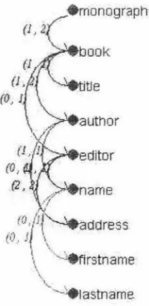
Let's look at the following XML document, reference.xml.

<monographs>

<book>

<title>Forever Xanadu</title>

<author>

<name>Hengren</name>

<address>1, Sesame Street</address>

</author>

<author>

<name>Gai</name>

<address>1, Sesame Street</address>

</author>

<editor>

<name>

<firstname>Lan</firstname>

<lastname>Zhou</lastname>

</name>

<address>2, Sesame Street</address>

<address>3, Sesame Street</address>

</editor>

</book>

<book>

<title>Eternal Bliss</title>

<author>

<name>li</name>

</author>

</book>

3.2. ER-XML EXTRACTION 23

Figure 3.2 shows the coloured ER-XML model diagram of reference.xml. 'monographs' is

the root element with 'book' as its sub-element, which in turn consists of 'title', 'author' and 'editor'. Both 'author' and 'editor' have sub-elements, 'name' and 'address'. 'name' is the parent of 'firstname' and 'lastname'. It is explicit that 'author' is both a base element, to 'name' and 'address' and non-base one, to 'book'. The cardinality information tells us that 'editor', 'address', 'firstname' and 'lastname' are optional (they may be unknown), indicated by the minimal occurrence of zero.

•monographs

(J,tr

\

author

editor

/t"' name

• I

,[

(

O

,

{If

--.

.

'

(0, j \

·, ',.~firstname

\

\.

--•1astname.

Figure 3.2: ER-XML Diagram Example

3.2 ER-XML Extraction

3.2.1

Depth-First Search (DFS) vs. Breadth-First Search (BFS)

DFS and BFS are the two core approaches to analyzing and processing connected graphs of vertices in computer science and other engineering disciplines.

CHAPTER 3. XML SCHEMA EXTRACTION 24

[Gross and Yellen, 1999]. DFS examines a frontier edge of the current vertex all the time until the end is reached and certain requirement is not met. Therefore, the algorithm, unless not possible, tends to go deeper in the graph. It is central to algorithms for solving connectivity and numerous other graph-processing problems.

BFS traverses the tree by always selecting frontier edges incident on vertices as close to the starting vertex as possible, i.e. all frontier edges from the starting vertex need to be considered in turn before looking at the next closest vertex. BFS considers all frontier edges of the current vertices prior to moving down the graph. It is mainly used for finding the shortest path between vertices.

A comparison example of DFS and BFS is more revealing:

DFS BFS

Figure 3.3: DFS and BFS Example(The number associated with each node indicates the sequence in which it is processed)

Both search algorithms maintain a list of edges to be recursively explored until it becomes empty. while both algorithms add items to the end of the list, the only difference is that BFS removes them from the beginning, which results in maintaining the list as a FIFO (First-in-First-out) queue, while DFS removes them from the end, maintaining the list as a stack.

3.2. ER-XML EXTRACTION

25

3.2.2 ER-XML Extraction (EXE) Algorithm

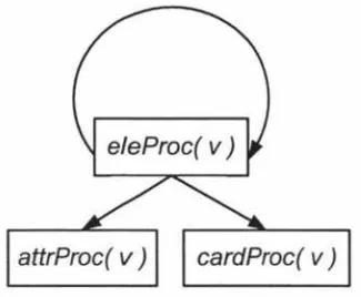
Required by distinct processing of elements and attributes, EXE is mainly composed of eleProc invoking attrProc accordingly. Figure 3.4 gives an overview of function calls between those methods:

e/eProc( v)

Figure 3.4: EXE Function Call Diagram

EXE is initialised by simply calling eleProc for the root:

Input: An XML Data tree TD with root r

Output: The corresponding ER- X ML model for Tv

/*

(1) eleProc(r);

CHAPTER 3. XML SCHEMA EXTRACTION 26

Input: An XML Data tree T0 and v E TD

Output: Schematic information of v and all its descendants

( 1) attr Proc( v); //process attributes

(2) if v is not a leaf then

(3) if not exist v' already processed of the same type as v then

( 4) Add v as a base element;

(5) Create its non-base element set N Bv;

(6) Filled N Bv with all v's child nodes CNi(l ~ i ~ m, m ~ 1);

(7) for each CNi EN Bv do

(8) Record Card(CNi) as for v;

(9) endfor

(10) else do

(11) cardProc(v); / /process cardinality information

(12) endif

/*

(13) for each CNi of v do

(14) eleProc(CNi);

(15) endfor

(16) else do //vis a leaf

(17) if v previously processed as a base element then (18) for each CNi EN Bv do

(19) Set lower bound of Card(CNi) to O;

(20) endfor

(21) else do

(22) Record v as a base element with empty N Bv;

(23) endif

(24) endif

3.2. ER-XML EXTRACTION

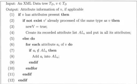
Input: An XML Data tree Tv, v E Tv

Output: Attribute information of v, if applicable

(1) if v has attributes present then

(2) if not exist v' already processed of the same type as v then (3) newV

=

( 4) Create its recorded attribute list ALv and put in all its attributes;

(5) else do

(6) for each attribute ai of v do

(7) if ai ff:. ALv then

(8) Add ai into ALv;

(9) endif

(10) endfor

(11) endif (12) endif

Figure 3.7: Method: attrProc( v )

CHAPTER 3. XML SCHEMA EXTRACTION

Input: An XML Data tree TD, v E TD and its child nodes, CNi(l:::;

i:::;

2:

(1) for each CNi do

(2) if exist its counter C( C Ni) then

(3) C(CNi)

=

+

(4) else do

(5) Initilise C(CNi) to 1;

(6) endif

(7) endfor

/*

* /

(9) if C Ni recorded as v's child before then

(10) Compare C(CNi) with Card(CNi) & adjust if needed;

(11) else do

(12) Add CNi into N Bv;

(13) Set its cardinality: (0, C(CNi));

(14) endif

(15) endfor

/*

(17) if not exist C(CNi) then

(18) Set it's cardinality lower bound to O; / /The C Ni is optional

(19) endif

(20) endfor

Figure 3.8: Method: cardProc( v )

Chapter 4

XML-Relation Data Transformation

There has been some research on transformation of XML data into relational structure

prompted by the growing demand from the industry, which however, due to the

com-plexity and difficulty, has not been satisfactorily catered for. In this section, we

con-trive a novel data transformation algorithm known as SVT-Trans to tackle the

prob-lem. We start off with some preliminary definitions upon which our algorithm is rooted

[Hartmann and Link, 2003, Hartmann et al., 2003].

4.1 Preliminary Definitions

4

.

1.

1

Root

e

d Tr

ee

and X

ML

Tr

ee

A rooted tree is a tree T with one distinguished vertex Rr as the root, such that every

vertex can be reached via a directed path from Rr and T contains neither directed nor

non-directed cycles. It is a common practice to illustrate the structure of an XML document

with the help of trees. For every tree T, let Vr denote its vertex set and Ar its arc set.

Definition 4.1.1. An XML tree is a rooted tree T together with mappings

name : Vr --+ Na mes, kind : Vr --+ { E, A} to assign every vertex its name and kind,

respectively. We suppose that Names is a fixed set of vertex names, whilst kind E and A

reveal whether a vertex actually represents either an element or an attribute. 0

In particular, Nv will be used wherever we refer to the name of vertex v.

CHAPTER 4. XML-RELATION DATA TRANSFORMATION 30

4.1.2

XML Schema Tree

Definition 4.1.2. An XML schema tree is an XML tree T in which no vertex has more

than one successor of the same name and the same kind. D

An XML schema tree can be interpreted as a graphical representation of the structure of

a native XML document, which may be easily generated either from the document itself

or its associated DTD. We refer to vertices in an XML schema tree as schema vertices.

4.1.3

XML Schema Tree Features

In a rooted tree, vertices of either kind A or E without successors are said to be leaves.

For simplicity, we focus on E-vertices in the rest of the chapter without loss of generality

in that A-vertices can be easily accommodated with slight adaptation. Moreover, textual

data attached to a non-leaf vertex is also not of interest to us.

Definition 4.1.3. Given a rooted tree T and any v, v' E Vr, a (v,v')-walk in terms ofT

is a directed walk from v to v'. D

It is evident that at most one (v, v')-walk can be found for a vertex pair (v, v') in T.

Throughout the paper, a (v, v')-walk is denoted by v ... v' due to the absence of confusion.

In particular, in the case where v becomes the root of T, i.e. Rr, this can be further eased

to rvv'.

In line with the structural flexibility of XML, i.e. different vertices may well have a child

vertex of the same name and type, we can pinpoint a vertex v by virtue of rvv for an

XML schema tree T with root Rr and v E T. Such an inspiration gives us the Universal

Naming Scheme to uniquely represent one vertex. The Universal Naming Scheme utilises

the name of all vertices on rvv partitioned by some delimiters. Take Figure 3.2 for

in-stance, there exist two different 'name' vertices, monographs$book$author$name1 _and

monographs$book$editor$name. This differentiation is vital since they represent distinct

semantics; 'author name' and 'editor name'. Where there is no such naming collision, we,

for conciseness, instead refer to vertices directly by their element name.

1_{The choice of delimiter $ is partially because it is one of few special characters fully supported by}

4.1. PRELIMINARY DEFINITIONS 31

Definition 4.1.4. Let LT be the set of all leaves in a rooted tree T. The v-subtree Tv for

vertex v in T is the union of all (v, w)-walks in T where w E LT. In addition, a c-subtree with c as an immediate successor of v is an offspring subtree of v-subtree. D

Note that any v-subtree of an XML schema tree is again an XML schema tree, which may well be just a single leaf vertex. We also refer to the complete leaf set of Tv as v-leafset Lv.

It is obvious that the union of two subtrees in T is again a subtree, which can be used to show that v-subtree is the union of all ci-subtrees corresponding to its N immediate successors Ci for 1 ::; i ::; N, which is also justified by an observation that all elements in v-leafset are distributed within some ci-subtree with 1 ::; i ::; N.

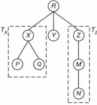
Example 4.1.1. Take for instance the XML schema tree T with root R presented in Figure 4.1. (X, P)-walk = X$P, (Z, N)-walk = Z$M$N and (R, M)-walk = R$Z$M, i.e. rvM. X-subtree Tx and Z-subtree Tz are enclosed by dashed line. In particular, Tx has two offspring subtrees Tp and TQ, i.e. leaf vertex P and Q.

TI

_x,

I

I I I

Figure 4.1: Schema tree, (v, v')-walk and v-subtree example

4.1.4

Mappings between XML Trees

CHAPTER 4. XML-RELATION DATA TRANSFORMATION 32

we regard </> name-preserving if name( v')

=

</> becomes a homomorphism between T and T' if the following conditions hold:

• R' is mapped to R, that is, </>(R')

=

• every arc in T' is mapped to an arc of T, that is, (

u'

,

v')

u'),

v'))

Ar,

• </> is kind-preserving and name-preserving.

Definition 4.1.5. A homomorphic 4> : Vr1 - Vr is an isomorphism if</> is bijective and

4>-i is also a homomorphism. In this case, we say T' is isomorphic to T or a copy of T.

Example 4.1.2. Consider XML tree Ti, T2 and T3 in Figure 4.2. Clearly, the

kind-preserving and name-preserving mapping 4> : Vr2 - Vn between T₂ and T₁ is homomor-phic in that the root and every arc in T2 are mapped to the correspondence in Ti. So is the mapping 4>' : Vr₃ - Vn. Moreover, T3 is isomorphic to Ti whilst it is not true in

terms of T2 and Ti; 4> is not bijective and nor is

4>-

Figure 4.2: Homomorphism and Isomorphism example

Definition 4.1.6. Let T and T' be two XML trees. An H'-subtree TlI, in T' is a subcopy

of T if it is a copy of some H-subtree TH in T. An almost copy of T, denoted by Or, is the maximal subcopy of T such that any other H" -subtree TlI,, in T', with Or C TlI,,, is

4.1. PRELIMINARY DEFINITIONS 33

Example 4.1.3. Figure 4-3 shows two XML trees T1 and T2 . It is easy to identify two

almost copies of T1 in T2 , each of which contains exactly one of the two D-subtrees in T2

and all other vertices.

Figure 4.3: Almost copy example

4.1.5

XML Data Tree

Definition 4.1.7. An XML data tree is an XML tree T together with an evaluation

val: Vr---+ STRING assigning every leaf a (possibly empty) string val(v). D

An XML data tree TD can be derived from the associated XML schema tree T by in-stantiating each schema vertex within. We refer to vertices in TD as instance vertices corresponding to some schema vertices in T correspondingly.

Definition 4.1.8. An XML data tree T' is said to be compatible with an XML schema tree T if the mapping </> : Vr, ---+ Vr is homomorphic.

4.1.6

Functional Dependencies for

XML

Functional dependency in XML(or XFD for short) is introduced by the following

CHAPTER 4. XML-RELATION DATA TRANSFORMATION 34

Definition 4.1.9. Let T be an XML schema tree with root R, a functional dependency is

an expression v: X - Y where X and Y are R-subtrees ofT. Let TD be an XML data tree

compatible with T. Then TD satisfies the XFD v : X - Y if for any two almost copies 01

and 0 2 of T in TD, the projections Oily and 0 2ly are equivalent whenever the projections

01lx and 02lx are equivalent and copies of X, i.e. 01 Ix

=

=

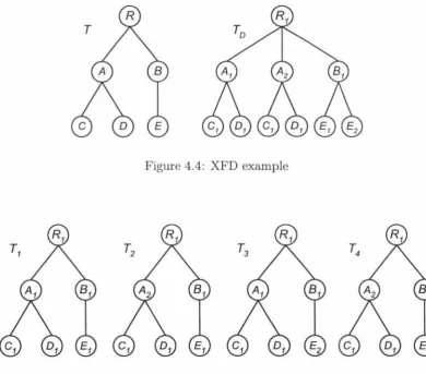
Example 4.1.4. Let us consider an XML schema tree T and its compatible XML data tree TD2 _{shown in Figure}

_4.4.

1 "' T4

(Figure

4-

all occurrences of C1 . In contrast, neither C - E nor D --+ E holds.

Figure 4.4: XFD example

Figure 4.5: XFD example (contd.) - identified almost copies

2_{We make it a convention to always label a schema vertex with an upper-case letter, say A, and its}

4.1. PRELIMINARY DEFINITIONS 35

4.1.7 Schema Vertex Table

Now we are ready to launch a crucial concept, schema vertex table (SVT for short), utilised as the basic building block in SVT-trans.

Definition 4.1.10. Consider an XML schema tree T, its entire leaf set Lr and an XML

data tree T' compatible with T, a schema vertex table SVT T for T is the consequence

of mappings schema : Lr --+ #SVTr and, for each almost copy of T presented in T',

value : val(£) --+ SVTr for each leaf /l, E Lr, to allocate to SVTr schema exactly one

column representing each leaf in Lr and to accommodate their associated textual values

from all almost copies of T, Or identified in T'. D

In particular, Sr refers to the entire set of SVTs for a schema tree T and all subtrees in

T.

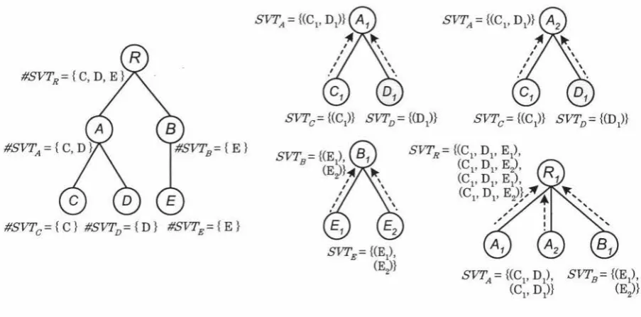
Example 4.1.5. Let us revisit the pair of XML schema and data tree in Figure

4.4.

SVTr contains 5 tables as shown in Figure

4.

(I)

,

(II)

of SVTr population with data from TD.

SVTA = {(C₁, D

1), SVT8= {(E1), (Cl' D

1)} (E2)}

I. ST schema determination II. ST data population

CHAPTER 4. XML-RELATION DATA TRANSFORMATION

36

We can see from the above example that each v-subtree is represented by a schema vertex

table SVTv, which is essentially in a two-dimension tabular format with each column representing a leaf in v-subtree. In particular, SVTg consists of one column only, with

column name as the element name of£, Ng E Names for any f E Le, as no leaf has

children but only textual data, which populates SVTe. It is also obvious that the semantic

information in each almost copy Ov of v-subtree in TD is captured by one single relation in SVTv due to the way the schemata of SVT, denoted by #SVT, is decided. For instance,

4 relations of SVTR in Example 4.1.5 correspond to those 4 almost copies in Figure 4.5 respectively.

Subsequently emerges an intuitive question - how their SVTs correlate for a P-subtree

and its offspring subtrees if any, the answer to which leads to:

Theorem 4.1.1. Let P-subtree be in a schema tree T(P E Vr) and Ci-subtrees

(1 ~ i ~ N) be its offspring subtrees, then #SVTp is the union of schema of all SVTci, N

i.e. #SVTp

=

LJ

i=l

of all SVTci, i.e. SVTp

=

Proof. As pointed out, the collaboration of all Ci-subtrees (1 ~ i ~ N) constitutes

P-subtree, whilst we know that a SVTv retains all structural and semantic information

presented in v-subtree from Definition 4.1.10. Thus substituting SVTv for v-subtree

( v E { P, Cl, C2, ... , C N}) justifies this proposition in two aspects: union operation in the

structural perspective and Cartesian join in the semantic perspective. The latter is deter-mined by the inference that no SVTci, SVTcj (if

j)

n

=I

0

originating from Definition 4.1.2. D

4.2

Tran

s

formation Methodology

By now, we are ready for the methodology in SVT-'Irans, the Schema Vertex Table Ma-nipulation approach by means of recursion developed based on Theorem 4.1.1, with the major processes of Initialisation and Population, and the operations Aggregation and Propagation. It applies to #SVT determination as well as SVT population. We will

4.2. TRANSFORMATION METHODOLOGY 37

• Initialisation process

Initialisation is conducted right at the beginning to decide the structure for Sr for an XML schema tree T, depending on type(v):

- For a leaf£, the leaf vertex name Nf. constitutes #SVTf. as previously

demon-strated.

- For a non-leaf v-subtree, #SVTv can be determined by recursively applying

Theorem 4.1.1 from the leaf level up, i.e. a bottom-up approach, with the help

of aggregation and propagation.

• Population process

After being set up, those SVTs then need to be populated with the semantic data

contained in all almost copies of corresponding subtrees identified in the data tree of the original XML document. Again, we start with SVTs at the leaf level, each of which in most cases holds only a single row3

- the textual data directly attached to the leaf itself. Sometimes, population of a leaf-level SVTf. may trigger aggregation if£ is the last (or only) child of its parent.

• Aggregation operation

Aggregation is a process in which a parent SVT is subsequently populated with the Cartesian product of all its child SVTs once they are done (a join operation),

or a parent #SVT is set by combining all its child #SVTs once they are done ( a

union operation). This is justified by the second half of Theorem 4.1.1. Aggregation always occurs at leaf level.

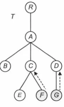
Example 4.2.1. Let us look at when aggregation happens to Sr of the schema tree T

in Figure

4-

table SVTF (as the last child of C) or SVTc (as the only child of D) will result in

aggregation leading to similar action on SVTc or SVTD correspondingly.

Under the subsequent circumstance, propagation comes into play:

- The parent vertex with its SVT populated or #SVT determined as a conse-quence of aggregation again is the last ( or only) child of its parent.

CHAPTER 4. XML-RELATION DATA TRANSFORMATION

38

Figure 4.7: Aggregation example

Example 4.2.2. The aggregation from G in Example 4.2.1 will give birth to a

propagation, indicated by an empty arrow in Figure

4.

parent D is also the last child of A.

Figure 4.8: Propagation example Figure 4.9: Greedy propagation example

• Propagation operation

As seen above, propagation takes place when some aggregation leads to further

aggregation. It bears the utmost significance as it 'glues' together aggregations

at multiple levels and pushes the whole SVT-processing up the XML schema tree

4.3. THE ALGORITHM SVT-TRANS 39

condition is again verified at the end of a propagation and, if satisfied, it is performed

repeatedly; the process persists until the propagation condition fails to hold, which

is now relaxed to:

- The parent vertex with its SVT populated or #SVT determined as a

conse-quence of aggregation ( or propagation) again is the last ( or only) child of its parent.

Example 4.2.3. The XML tree from the previous example also demonstrates propagation being 'greedy'. Figure

4.

4.3 The Algorithm SVT-Trans

The algorithm SVT-Trans is introduced in full detail here. Figure 4.10 firstly presents an

overview of SVT-Trans covering its structure and all methods which we will have a closer

look at in turn.

4.3.1

SVT-Trans Overview

Given an XML document X, its data tree TD 4 _{with root r, its schema tree T with root}

R and the entire leaf set Lr as a result of applying the EXE algorithm, SVT-Trans is

composed of two primary methods, setSVT(v) and populateSVT(v, v) with both utilising recursion by essentially starting with R( and r):

• setSVT(v)

This method corresponding to the initialisation process determines and establishes a

SVTv for every schema vertex v E T. It then recursively calls itself for every child of

v in sequence until reaching a leaf£, at which #SVTe is set to Ne E Names. Aggre-gation or propaAggre-gation takes place whenever their condition is satisfied. setSVT( v)

terminates when #SVTv is eventually settled(Figure 4.11 & Figure 4.12).

4_{TD can be conveniently acquired with the help of an XML parser. Detail is discussed at an appropriate}

CHAPTER 4. XML-RELATION DATA TRANSFORMATION Input: T, R, TD, r, Lr

Output: the SVTR fully populated with all semantic data from X

/*

/*

(2) Create all SVTs using Database Definition Language(DDL);

/*

(3) populateSVT(R, r);

Figure 4.10: Algorithm: SVT-'Irans

• populateSVT(v, v)

40

This method corresponding to the population process retrieves and transforms the

semantic data bound in X into the SVT R to be used in the X F D discovery analysis

later. It recursively calls itself for v's every child c, together with every almost copy of c in TD, represented by an instance vertex

c;,

c;)

reaching the leaf level (£, l), at which SVTe is packed with the textual data attached

to l. Aggregation or propagation takes place whenever their condition is satisfied.

populateSVT(v, v) terminates when SVTv is eventually populated.

A schema vertex v and its every instance vertex v E TD is paired up as the

parame-ters here since SVTv need to convene the semantic information held in every almost copy of v-subtree, i.e. the corresponding v-subtree in TD. Hence it is essential to

keep track of the schema-instance vertex correspondence(Figure 4.13, Figure 4.14

& Figure 4.15).

As seen from Figure 4.16, recursion plays a significant role in both methods, partially

empowered by XML schema tree and data tree, both a rooted tree. With the root as the

starting point, recursion pushes the processing down and then up the tree to determine

and populate SVTs - a 'top-down-up' fashion.

Compactness and high reusability is another feature of SVT-'Irans attributed to the

in-novative concept of SVT; an SVTv corresponds to the v-subtree in an XML schema tree

and deals with all its almost copies in a compatible XML data tree. This also explains

4.3. THE ALGORITHM SVT-TRANS

Input: T,Tv,R,v ET

Output: #SVTv

/*

(1) if v E Lr then

(2)

=

//v is a leaf

/ II

I=

(4) if satisfied then

(5) aggregateSetSVT( v );

(6) endif

/*

(7) else do / / v is an internal vertex

(8) for each child c of v do

(9) setSVT(c); //recursion

(10) endfor

(11) endif

Figure 4.11: Method: setSVT( v )

Input: T, R, Tv, r, Lr

Output: the SVTn fully populated with all semantic data from X

(1) Union #SVTv (and all its sibling #SVTs) into #SVTp; //p is v's parent

(2) Check against propagation condition; (3) if satisfied then

(4) aggregateSetSVT(p); //recursion

(5) endif

Figure 4.12: Method: aggregateSetSVT( v )

41

CHAPTER 4. XML-RELATION DATA TRANSFORMATION

Input: T, TD, R, v ET, v E TD of type v Output: Populated SVTv

/*

(1) if v E Lr then //v is a leaf

(2) insert val(£) into SVTv;

(3) check against aggregation condition; ( 4) if satisfied then

(5) aggregatePopSVT(v,

v);

(6) endif

/*

(7) else do

//v

(8) for each child c of v do

(9) check for all CD E T0 of type c attached directly to v; (10) if any CD then

(11) for each cD do

(12) populateSVT(c, c0 ); //recursion

(13) endfor

( 14) else / / c is not presented under v E TD (15) populate SVTc with NULL;

(16) check against aggregation conditions; ( 17) if satisfied then

(18) aggregatePopNullSVT(c, v);

(19) endif

(20)

(21) endfor

(22) endif

Figure 4.13: Method: populateSVT( v, v)

4.3.2 Handling NULL Values

42

As a highly functional subset of SGML, the popularity XML enjoys is to a large extent

4.3. THE ALGORITHM SVT-TRANS

(1) Join SVTv (with all its sibling SVTs) into SVTp; / / p is the parent of V

(2) Empty SVTx for every x E p-subtree and x

=J

(3) Check against propagation condition;

(4) if satisfied then

(5) for v's parent PDE TD do

(6) aggregatePopSVT(p, p D); / /recursion

(7) endfor

(8) endif

Figure 4.14: Method: aggregatePopSVT( v, v )

(1) Join SVTc (with all its sibling SVTs) into SVTv; //v is the parent of c (2) Empty SVTx for every x E v-subtree and x =I= v;

(3) Check against propagation condition;

( 4) if satisfied then

(5) aggregatePopSVT(v, v);

(6) endif

Figure 4.15: Method: aggregatePopNullSVT( c, v )

setSVT( v)

Figure 4.16: SVT-Trans Function Call Diagram