Multigrid Algorithm Based on Hybrid Smoothers for Variational and Selective Segmentation Models

A Multigrid Algorithm with Non-Standard Smoother for

Two Selective Models in Variational Segmentation

M

ichael

R

oberts

, K

e

C

hen

and

K

laus

I

rion

†_{Centre for Mathematical Imaging Techniques and Department of Mathematical}

Sciences, The University of Liverpool, United Kingdom

and

Liverpool, United Kingdom

Abstract

Automatic segmentation of an image to identify all meaningful parts is one of the most challeng-ing as well as useful tasks in a number of application areas. This is widely studied. Selective segmentation, less studied, aims to use limited user specified information to extract one or more interesting objects (instead of all objects). Constructing a fast solver remains a challenge for both classes of model. However our primary concern is on selective segmentation.

In this work, we develop an effective multigrid algorithm, based on a new non-standard smoother to deal with non-smooth coefficients, to solve the underlying partial differential equations (PDEs) of a class of variational segmentation models in the level set formulation. For such models, non-smoothness (or jumps) is typical as segmentation is only possible if edges (jumps) are present. In comparison with previous multigrid methods which were shown to produce an acceptablemeansmoothing rate for related models, the new algorithm can ensure a small and

globalsmoothing rate that is a sufficient condition for convergence. Our rate analysis is by Local Fourier Analysis and, with it, we design the corresponding iterative solver, improving on an ineffective line smoother. Numerical tests show that the new algorithm outperforms multigrid methods based on competing smoothers.

Keywords. Partial differential equations, multigrid, fast solvers, Local Fourier Analysis, image segmentation, jump coefficients.

1.

I

ntroduction

Segmentation of an image into its individual objects is one incredibly important application of image processing techniques. Not only are accurate segmentation results required, but also it is required that the segmentation method is fast. Many imaging applications demand increasingly higher resolution e.g. an image of size 25000 × 25000 (or practically 108 unknowns) can be common in oncology imaging. Here we address the problem of slow solutions by developing a fast multigrid method for PDEs arising from segmentation models.

Segmentation can take two forms; firstly global segmentation is the isolation of all objects in an image from the background and secondly, selective segmentation is the isolation of a subset of the objects in an image from the background. Selective segmentation is very useful in, for example, medical imaging for the segmentation of single organs.

∗

Email [email protected], Web: www.liv.ac.uk/cmit (corresponding author). Work supported by UK EPSRC grant EP/K036939/1.

Approaches to image segmentation broadly fall into two classes; region-based and edge-based. Some region-based approaches are region growing [1], watershed algorithms [37], Mumford-Shah [26] and Chan-Vese [15]. The final two of these are PDE-based variational approaches to the problem of segmentation. There are also models which mix the two classes to use the benefits of the region-based and edge-based approaches and will incorporate features of each. Edge-based methods aim to encourage an evolving contour towards the edges in an image and normally require an edge detector function [12]. The first edge-based variational approach was devised by Kass et al. [21] with the famous snakes model, this was further developed by Casselles et al. [12] who introduced the Geodesic Active Contour (GAC) model. Region-based global segmentation models include the well known works of Mumford-Shah [26] and Chan-Vese [15]. Importantly they are non-convex and hence a minimiser of these models may only be a local, not the global, minimum. Further work by Chan et al. [14] gave rise to a method to find the global minimiser for the Chan-Vese model under certain conditions.

Selective segmentation of objects in an image, given a set of points near the object or objects to be segmented, builds in such user input to a model using a setS = {(xi,yi) ∈ Ω, 1≤ i ≤ k} whereΩ⊂R2_{is the image domain [19, 5, 6]. Nguyen et al. [28] considered marker setsS and} Awhich consist of points inside and outside, respectively, the object or objects to be segmented. Gout et al. [19] combined the GAC approach with the geometrical constraint that the contour pass through the points ofS. This was enforced with a distance function which is zero atS and non-zero elsewhere. Badshah and Chen [5] then combined the Gout et al. model with [15] to incorporate a constraint on the intensity in the selected region, thereby encouraging the contour to segment homogenous regions. Rada and Chen [30] introduced a selective segmentation method based on two-level sets which was shown to be more robust than the Badshah-Chen model. We also refer to [6, 22] for selective segmentation models which include different fitting constraints, using coefficient of variation and the centroid ofS respectively.

None of these models have a restriction on the size of the object or objects to be detected and depending on the initialisation these methods have the potential to detect more or fewer objects than the user desired. To address this and to improve on [30], Rada and Chen [31] introduced a model (we refer to it as the Rada-Chen model from now on) combining the Badshah-Chen [5] model with a constraint on the area of the objects to be segmented. The reference area used to constrain the area within the contour is that of the polygon formed by the markers inS. Spencer and Chen [33] recently introduced a model with the distance fitting penalty as a standalone term in the energy functional, unbounding it from the edge detector term of the Gout et al. model. All of the above selective segmentation models discussed are non-convex and hence the final result depends on the initialisation. Spencer and Chen [33], in the same paper, reformulated the model they introduced to a convex form using a penalty term as in [14]. We have considered the convex Spencer-Chen model but found that the numerical implementation is unfortunately sensitive to the main parameters and is unstable if they aren’t chosen correctly within a small range; hence we focus on the non-convex model they introduce for which reliable results have been found (we refer to this as the Spencer-Chen model from now on). A convex version of the Rada-Chen model cannot be formulated [33]. In this paper we only consider 2D images, however for completion we remark that 3D segmentation models do exist [23, 39].

the system is equal to the number of pixels in the image, which can be very large, and for each equation in the system the number of steps of an iterative method required can also be very large (to reach convergence). Due to improvements in technology and imaging, we now can produce larger and larger images, however this has the direct consequence that analysis of such images has become much more computationally intensive. We remark that if we directly discretise the variational models first (without using PDEs), Chan-Vese type models can be reformulated into minimisation based on graph cuts and then fast algorithms have been proposed [7, 25].

The multigrid approach for solving PDEs in imaging has been tried before and previous work by Badshah and Chen [3, 4] introduced a 2D Chan-Vese multigrid algorithm for two-phase and multi-phase images, additionally Zhang et al. [39] implemented a multigrid algorithm for the 3D Chan-Vese model. The fundamental idea behind multigrid is that if we perform most of the computations on a reduced resolution image then the computational expense is lower. We then transfer our solution from the low resolution grid to the high resolution grid through interpolation and smooth out any errors which have been introduced by the interpolation using a few steps of a smoothing algorithm, e.g. Gauss-Seidel. The multigrid method is an optimal solver when it converges [24, 34]. This requires that the smoothing scheme, which corrects the errors when transferring between the higher and lower resolution images and vice-versa, is effective, i.e. reduces the error magnitude of high-frequency components quickly.

In the large literature of multigrid methods, the convergence problem associated with non-smooth or jumping coefficients was often highlighted [2, 11] and developing working algorithms which converge is a key problem. Much attention was given to designing better coarsening strategies and improved interpolation operators [38, 40] while keeping the simple smoothers; such as the damped Jacobi, Gauss-Seidel or line smoothers. In practice, one can quickly exhaust the list of standard smoothers and yet cannot find a suitable one unless compromising in optimality by increasing the number of iterations. In contrast, our approach here is to seek a non-standard and more effective smoother with an acceptable smoothing rate. Our work is motivated by Napov and Notay [27] who established the explicit relationship of a smoothing rate to the underlying multigrid convergence rate for linear models; in particular the former also serves as the lower bound for the latter.

The contributions of this paper can be summarised as follows: (1) We review six smoothers for the Rada-Chen and Spencer-Chen selective segmentation models and perform Local Fourier Analysis (LFA) to assess their performance and quantitatively determine their effectiveness (or lack of). (2) We propose an effective non-linear multigrid method to solve the Rada-Chen model [31] and the Spencer-Chen model [33], based on a new smoothers that add non-standard smoothing steps locally at coefficient jumps. We recommend in particular one of our new hybrid smoothers which achieves a better smoothing rate than the other smoothers studied and thus gives rise to a multigrid framework which converges to the energy minimiser faster than when standard smoothers are used.

analyse the complexity of the recommended multigrid algorithm. Finally in §6 we provide some concluding remarks.

2.

R

eview of segmentation models

Our methods will apply to both global segmentation models and selective segmentation models. It is necessary to briefly describe both types. Denote a given image in domainΩ⊂R2_byz(x,y).

2.1.

Global segmentation models

The model of Mumford and Shah [26] is one of the most famous and important variational models in image segmentation. We will review its two-dimensional piecewise constant variant, commonly known as the Chan-Vese (CV) model [15], which takes the form

min Γ,c1,c2

FCV(Γ,c1,c2) =µ·length(Γ) +λ1

Z

Ω1

|z(x,y)−c1|2dΩ+λ2

Z

Ω2

|z(x,y)−c2|2dΩ (1)

where the foreground Ω1 is the subdomain to be segmented, the background isΩ2 = Ω\Ω1

andµ,λ1,λ2are fixed non-negative parameters. The valuesc1andc2are the average intensities

ofz(x,y)insideΩ1andΩ2respectively. Using the ideas of Osher and Sethian [29], a level set

function

φ(x,y) =

  

 

>0, (x,y)∈Ω1,

0, (x,y)∈Γ,

<0, otherwise,

is used by [15] to track the object boundaryΓ, where we now define it as the zero level set ofφ, i.e.

Γ={(x,y)∈Ω|φ(x,y) =0}. We reformulate (1) as

min φ,c1,c2

FCV(φ,c1,c2) =µ

Z

Ω|∇Hε(φ)|dΩ+λ1 Z

Ω(z(x,y)−c1) 2_H

ε(φ)dΩ

+λ2

Z

Ω(z(x,y)−c2)

2_(1−H

ε(φ))dΩ,

(2)

with Hε(φ)a smoothed Heaviside function such as [15]

Hε(φ) = 1

2 +

1

πarctan

φ

ε

where we useε=1 in our experiments. We solve this minimisation problem in two stages, first

withφfixed we minimise with respect toc1andc2, yielding

c1=

R

ΩHε(φ)·z(x,y)dΩ R

ΩHε(φ)dΩ

, c2=

R

Ω(1−Hε(φ))·z(x,y)dΩ R

Ω(1−Hε(φ))dΩ

, (3)

and secondly, withc1andc2fixed we minimise (2) with respect toφ. This requires the

2.2.

Selective segmentation models

Selective segmentation models make use of user input, being a marker set of points near the object or objects to be segmented. LetS ={(xi,yi)∈Ω, 1≤i≤k}be such a marker set. The contour is encouraged to pass through or near the points ofS by a distance function such as [23]

d(x,y) =

k

∏

1−e−

(_xi−x)2 2σ2 e−

(_yi−y)2 2σ2

, ∀(x,y)∈Ω,(xi,yi)∈ S,

whereσ is a fixed non-negative tuning parameter. See, for example, [19, 33] for other distance

functions. The distance function is zero at the points of S and non-zero elsewhere, taking a maximum value of one. Gout et al. [23] were the first to introduce a model incorporating a distance function into the Geodesic Active Contour model of Caselles et al. [12], however this model struggles when boundaries between objects and their background are fuzzy or blurred. To address this, Badshah and Chen [5] introduced a new model which includes the intensity fitting terms from the CV model (1). However this model has poor robustness [30] if iterating for too many steps the final segmentation can include more or fewer objects than intended. To improve on this, Rada and Chen [31] introduced a model which incorporates an area fitting term into the Badshah-Chen (BC) model and is far more robust.

The Rada-Chen model[31]. This is the first model we focus on in this paper, defined by

FRC(φ,c1,c2) =µ

Z

Ωd(x,y)g(|∇z(x,y)| 2_)|∇H

ε(φ)|dxdy

+λ1

Z

Ω(z(x,y)−c1) 2_H

ε(φ)dxdy+λ2

Z

Ω(z(x,y)−c2)

2_(1−H

ε(φ))dxdy

+ν

Z

ΩHε(φ)dxdy−A1 2

+

Z

Ω(1−Hε(φ))dxdy−A2 2

,

(4)

whereµ,λ1,λ2,νare fixed non-negative parameters. The edge detector function g(|∇z(x,y)|2)is

given byg(s) =1/(1+βs)for tuning parameterβwhich takes value 0 at edges and is 1 away

from them. A1is the area of the polygon formed from the points ofS and A2=|Ω| −A1. The

final term of this functional therefore puts a penalty on the area inside a contour being very different toA1. The first variation of (4) with respect toφgives the Euler-Lagrange form [31]

δε(φ)

µ∇ ·

d(x,y)·g(|∇z(x,y)|2_)∇

φ

|∇φ|

−hλ1(z(x,y)−c1)2−λ2(z(x,y)−c2)2 i

−ν

(

Z

ΩHε(φ)dxdy−A1)−( Z

Ω(1−Hε(φ))−A2)

=0,

(5)

inΩwith the condition that ∂φ

∂n =0 on∂Ω,nthe outward normal vector andδε(φ) = dHε(φ)

dφ .

Discretisation of the Rada-Chen model. We denote byφi,j =φ(xi,yj)the approximation ofφat

(i,j)for 1≤i≤nand 1≤j≤m. We lethxandhybe the grid spacings in thexandydirections respectively. Using finite differences, and notingA2=1−A1, we obtain the scheme

Ai,jφi+1,j+Bi,jφi−1,j+Ci,jφi,j+1+Di,jφi,j−1−Si,jφi,j

−δε(φi,j)

λ1(zi,j−c1)2−λ2(zi,j−c2)2

−2ν

hxhy

∑

k,l

Hε(φk,l)−A1

where Gi,j=

di,j·g(|∇zi,j|)

|∇φi,j|

, Ai,j =

µδε(φi,j)

h2

x

G_i+1

2,j, Bi,j=

µδε(φi,j)

h2

x

G_i−1 2,j,

Ci,j=

µδε(φi,j)

h2

y

G_i,j+1

2, Di,j =

µδε(φi,j)

h2

y

G_i,j−1

2, Si,j =Ai,j+Bi,j+Ci,j+Di,j, (7)

The Spencer-Chen model[33]. The second model we focus on in this paper is defined by

FSC(φ,c1,c2) =µ

Z

Ωg(|∇z(x,y)| 2_)|∇H

ε(φ)|dxdy+λ1

Z

Ω(z(x,y)−c1) 2_H

ε(φ)dxdy

+λ2

Z

Ω(z(x,y)−c2)

2_(1−H

ε(φ))dxdy+θ

Z

Ωd(x,y)Hε(φ)dxdy,

(8)

whereµ,λ1,λ2andθare fixed non-negative parameters. Note that this model differs from the

Rada-Chen model (4) as the distance function has been separated from the edge detector term and is now a standalone penalty term. This model has Euler-Lagrange form

δε(φ)

µ∇ ·

g(|∇z(x,y)|2_)∇φ |∇φ|

−hλ1(z(x,y)−c1)2−λ2(z(x,y)−c2)2 i

−θd(x,y)

=0, (9)

inΩwith the condition that ∂φ_∂n =0 on∂Ω, again withnthe outward normal vector. We discretise

this similarly to the Rada-Chen model previously.

3.

N

on

-

linear multigrid

A

lgorithm

1

Segmentation using a non-linear multigrid algorithm has been explored by Badshah and Chen [3, 4] for the Chan-Vese model [15] and the Vese-Chan model [36] which are global segmentation models. A multigrid method has not yet been applied to selective segmentation and this is the main task of this paper, to apply the multigrid method to the Rada-Chen (4) and Spencer-Chen (8) selective segmentation models. However as we will see shortly, the task is challenging as standard methods do not work. For brevity we will restrict consideration just to the Rada-Chen model as the derivations for the Spencer-Chen model are similar.

3.1.

The Full Approximation Scheme

To solve the Rada-Chen model we must solve the non-linear system (6) and so we will use the non-linear Full Approximation Scheme [13, 16, 20, 34] algorithm due to Brandt [9]. Denote a discretised system by

Nhφh= fh, (10)

whereh indicates that these are the functions on then×mcell-centred gridΩh andNhis the discretised non-linear operator (which contains the boundary conditions). Similarly define the gridsΩ2has the n₂×m₂ cell-centred grid resulting from the standard coarsening [34] ofΩh, we indicate functions onΩ2h by f2h,N2handφ2h. LetΦh be an approximation toφhsuch that the

erroreh =φh−Φh is smooth. Define the residual asrh = fh−NhΦh. Therefore using (10) we

have the residual equation

If the errorehissmooththen this can be well approximated onΩ2h; the assumption can be a big issue for non-linear problems. With an approximation of eh onΩ2hwe can solve the residual equation onΩ2h, which is significantly less computationally expensive than solving onΩh, and then transfer this error toΩhand use it to correct the approximationΦh. This method, using the two gridsΩ2handΩh, is called a two-grid cycle and it can be nested such that we can consider solving onΩ4h_,Ω8h_{, . . . and transferring the errors up through the levels toΩ}h_{and smoothing on} each level. This is the multigrid method. We transfer fromΩhtoΩ2hby restriction and fromΩ2h toΩhby interpolation.

Restriction. We use the full-weighting operatorI2h

h Φh=Φ2h[34]

φ_i2_,h_j = 1

16

h

φh_2i−1,2j−1+2φh2i−1,2j+φ2hi−1,2j+1+2φ2hi,2j−1+4φ2hi,2j

+2φh_2i,2j+1+φ₂h_i+1,2j−1+2φ₂h_i+1,2j+φh_2i+1,2j+1

i

,

and at boundary pixelsφ2_i,h_m= 1₂

h

φh_2i,m−1+φh_2i,m

i

andφ2_nh_,j= 1₂

h

φh_n−1,2j+φh_n,2j

i

.

Interpolation. We use a bilinear interpolation operatorI₂h_hΦ2h=Φh[34]

φ₂h_i,2j=φ_i2_,h_j, φ₂h_i+1,2j = 1

2

h

φ2_i,h_j +φ2_i+h_1,j

i

, φh_2i,2j+1= 1

2

h

φ2_i,h_j +φ2_i,h_j+1

i

,

φ₂h_i+1,2j+1= 1

4

h

φ_i2_,h_j +φ_i2₊h_1,j+φ_i2_,h_j+1+φ2_i+h_1,j+1

i

.

We now move to the most important element of the multigrid method – the smoother. As previously mentioned, we needehto be smooth to ensure thatΦhis a good approximation toφh.

In practice, we smoothehby using an iterative method such as Gauss-Seidel [3, 4] and the success or failure of a multigrid method hinges on the effectiveness of it at smoothing the errors.

3.2.

Smoothers for the Rada-Chen [31] model

Gauss-Seidel and Newton iterative methods have been shown to be effective smoothers for PDE problems with smooth coefficients [34, 38]. In this subsection we look at three distinct smoothing iterative techniques; lexicographic Gauss-Seidel, line Gauss-Seidel and Newton smoothers. For each of these smoothers we consider two different approaches for fixing the coefficients in the scheme - globally or locally. Hence overall we consider six smoothers for [31]; the same smoothers are adaptable for [33] in a simple way.

Smoothers 1-2 (GSLEX I - II). Lexicographic Gauss-Seidel smoothers are widely used in multigrid

methods [3, 34]. We updateφi,jone at a time and work across and down through the grid of pixels in an image.Lexicographic Gauss-Seidel smoothers for the Rada-Chen model[31]. We can rearrange (6) as

φi,j = Ai,jφi+1,j+Bi,jφi−1,j+Ci,jφi,j+1+Di,jφi,j−1− fi,j Si,j, (11)

where fi,j =δε(φi,j)

n

λ1(zi,j−c1)2−λ2(zi,j−c2)2+2ν+hxhy∑k,lHε(φk,l)−A1 o

pixel(i,j)in turn solving (11) and updating the value ofφ(i,j), only with GSLEX-II do we update

the coefficients immediately and they are used in the update ofφ(i,j)on the next iteration.

Smoothers 3-4 (GSLINE I - II). Line smoothers are often used for harder problems (e.g. anisotropic

coefficients). Here we perform the Gauss-Seidel updates one column at a time but the approach can be easily reformulated for a row by row update.

Gauss-Seidel line smoothers for the Rada-Chen model[31]. If we rearrange (6) to have all theφ·,jterms on the left hand side we obtain

Ai,jφi+1,j+Bi,jφi−1,j−Si,jφi,j =Fi,j =−Ci,jφi,j+1−Di,jφi,j−1+fi,j, (12)

where we can reformulate (12) as the following tridiagonal system



























−

S

A

0

. . .

0

0

B

−

S

A

. ..

0

0

0

B

. ..

. ..

. ..

..

.

..

.

. ..

. ..

. ..

A

0

0

0

. ..

B

−

S

A

0

0

. . .

0

B

−

S



























·



























φ

φ

..

.

..

.

φ

φ



























=



























F

F

..

.

..

.

F

F



























.

This system is diagonally dominant (by definition (7)) and if Ci,j+Di,j 6= 0 then the system is strictly diagonally dominant. We can choose parameters for the edge detector and distance function which ensure this is always true. Therefore this will ensure that the Gauss-Seidel line smoother will converge to a solution [18]. As before, we obtain two smoothers; the global smoother GSLINE-I and the local smoother GSLINE-II.

Smoothers 5-6 (NEWT I - II). Our last set of smoothers rely on the Newton fixed point iteration

schemes.

Newton smoothers for the Rada-Chen model[31]. We can rewrite (6) in a non-linear form forφi,j

Si,jφ(_i,k_j)−Pi,j+Qi,j(φ(_i,k_j)) =0.

where Pi,j = Ai,jφi+1,j+Bi,jφi−1,j+Ci,jφi,j+1+Di,jφi,j−1−δε(φi,j)

λ1(zi,j−c1)2−λ2(zi,j−c2)2

andQi,j =2νδε(φi,j)hxhy∑k,lHε(φk,l)−A1. The Newton scheme to computeφ(_i,k_j+1)is

φ_i(_,k_j+1)=φ_i(_,k_j)− Si,jφ(_i,k_j)−Pi,j+Qi,j(φ_i(_,k_j)) Si,j+Q0i,j(φ (k) i,j )

(14)

whereQ0_i,j(φ_i(_,k_j)) =2νδε(φi,j)2hxhy+2νδ_ε0(φi,j))

h

hxhy∑k,lHε(φk,l)−A1 i

. We again have a global smoother, NEWT-I, and a local smoother, NEWT-II.

3.3.

Algorithm 1

Algorithm 1:FAS multigrid algorithm,φh←FASMG(φh,Nh,fh,γ,ν1,ν2,level,max_level,Smoother)

Pre-smoothing:Performν1iterations of the smoother: φh←Smoother(φh,fh,ν1).

Coarse grid correction: Compute the residual: rh= fh−Nhφh.

Transfer the residual toΩ2hby restriction: r2h=I_h2hrh.

Compute: φ2h=I_h2hφh,Φ2h=φ2h,f2h=N2hφ2h+r2h.

iflevel=max_levelthen

Compute the exact solutionφ2hofN2h(φ2h) =N2h(Φ2h) +r2h

onΩ2husing e.g. time-marching [15] or AOS [34]. else

Performγcycles (steps) of

φ2h←FASMG(φ2h,N2h,f2h,γ,ν1,ν2,level+1,max_level,Smoother).

end if

Interpolation: Compute: e2h₌

φ2h−Φ2h.

Transfer the error toΩhby interpolation: eh=I₂h_he2h. Correct the fine grid approximation: φh=φh+eh.

Post-smoothing:Performν2iterations of the smoother: φh←Smoother(φh,fh,ν2).

3.4.

Local Fourier Analysis of Algorithm 1 for the Rada-Chen Model

Local Fourier Analysis (LFA) is a useful tool for finding a quantitative measure for the effectiveness of a smoother [9, 16, 34]. It is designed to study linear problems with constant coefficients on an infinite grid. However, it is a standard and recommended [9, 11] tool to analyse non-linear operators. To overcome the limitations, we neglect the boundary conditions, extend the operator to an infinite grid and assume that we can linearise the operator locally (we do this by freezing the coefficients). LFA measures the largest amplification factor on high-frequency errors, for example if there is a smoothing rate of 0.8 this means that the high-frequency errors are damped by at least 20%. We initially must derive formulas for the approximation error at each pixel in our 5-point stencil.

Error forms.Using the definition of fi,j, we can rewrite (6) as

Ai,jφi+1,j+Bi,jφi−1,j+Ci,jφi,j+1+Di,jφi,j−1−Si,jφi,j= fi,j, (15)

where we fixAi,j,Bi,j,Ci,jandDi,jbased on a previous iteration. The GSLEX I-II and NEWT I-II schemes all work in a lexicographic manner, and so if we denote the previous iteration as thek-th we can rewrite (15) as

Ai,jφ_i(₊k)_1,j+Bi,jφ_i(₋k+_1,1_j)+Ci,jφ_i(_,k_j)₊₁+Di,jφ_i(_,k_j+₋₁1)−Si,jφ_i(_,k_j+1)= fi,j, (16)

and we obtain the error form by subtracting (16) from (15)

Ai,je(_i+k)_1,j+Bi,je(_i−k+1,1j)+Ci,je (k)

i,j+1+Di,je

(k+1) i,j−1 −Si,je

(k+1)

i,j =0, (17)

Using a similar argument, we obtain the following error form for the line smoothers GSLINE I-II

Ai,je(_i+k+_1,1_j)+Bi,je_i(−k+1,1j)+Ci,je (k)

i,j+1+Di,je

(k+1) i,j−1 −Si,je

(k+1)

wheree(_i,k_j)=φi,j−φ_i(_,k_j)ande_i(_,k_j+1)=φi,j−φ_i(_,k_j+1).

Local Fourier Analysis. Define a general Fourier component by

Fθ1,θ2(xi,yj) =exp

2πiθ1i

n

·exp

2πiθ2j

m

=exp

iα1xi

hx

·exp

iα2yj

hy

,

where α1 = 2θn1π andα2 = 2θm2π andi is the imaginary unit. Note that α1,α2 ∈ [−π,π]. If we

assume for simplicity that the image is square and hencen=m, we first expand

e(_i,k_j+1)=

n/2

∑

θ1,θ2=−n/2

ψ(_θk+1)

1,θ2 Fθ1,θ2(xi,yj), e (k) i,j =

n/2

∑

θ1,θ2=−n/2

ψ(_θk)

1,θ2Fθ1,θ2(xi,yj),

in Fourier components and define the smoothing rate ˆµi,jby [34, 16]

ˆ

µi,j=max θ1,θ2

µ(θ1,θ2) =max

θ1,θ2

ψ_θ(k+1)

1,θ2

ψ(_θk)

1,θ2

,

in the high-frequency range where(α1,α2) = (2θn1π,

2θ2π

n )∈[−π,π)2\[−π2,π2)2. Since ˆµi,jis pixel

dependent (non-linear problems), we may also call it the amplification factor associated with(i,j).

Smoothing rates.For the GSLEX I-II, NEWT I-II smoothers, using (17) and (18), we obtain error

amplification at pixel(i,j)

ˆ

µi,j =max θ1,θ2

µ(θ1,θ2) =max

α1,α2

Ai,jeiα1+Ci,jeiα2

Bi,je−iα1+Di,je−iα2−Si,j

,

and similarly for the GSLINE I-II smoothers we have

ˆ

µi,j=max θ1,θ2

µ(θ1,θ2) =max

α1,α2

Ci,jeiα2

Ai,jeiα1+Bi,je−iα1+Di,je−iα2−Si,j

. (19)

Comparison of smoothing rates for all smoothers. We consider two different measures of the

smoothing rates; the maximum and average over all pixels(i,j). We define these in the obvious way as

˜

µmax=max

i,j µˆi,j=maxi,j maxθ1,θ2

µ(θ1,θ2) and µ˜avg=

∑i,jµˆi,j

n2 =

∑i,jmaxθ1,θ2µ(θ1,θ2)

n2 .

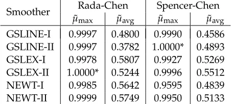
Each of the smoothers was implemented in Algorithm 1 on the image in Figure 1(a) with a V-cycle (γ =1) and using a 1024×1024 resolution image as the finest grid and a 32×32 image as the

coarsest grid and in Table 1 we give ˜µmaxand ˜µavgfor the Rada-Chen and Spencer-Chen models.

In the spirit of previous works [3], for any of these smoothers, one would quote ˜µavg, and although

this appears to be an excellent rate in all cases, it is the rate ˜µmaxthat determines the multigrid

convergence [27]. We therefore choose to focus on ˜µmax. Table 1 shows us that ˜µmaxis better for

Smoother Rada-Chen Spencer-Chen ˜

µmax µ˜avg µ˜max µ˜avg

GSLINE-I 0.9997 0.4800 0.9990 0.4586

GSLINE-II 0.9997 0.3782 1.0000* 0.4893

GSLEX-I 0.9978 0.5807 0.9927 0.5269

GSLEX-II 1.0000* 0.5244 0.9996 0.5512

NEWT-I 0.9985 0.5642 0.9595 0.4839

NEWT-II 0.9999 0.5749 0.9950 0.5133

Table 1:Smoothers and the associated maximum and average smoothing rates for the Rada-Chen and Spencer-Chen models. * due to rounding.

next section we will see that the problem is due to discontinuous coefficients in the numerical schemes, and so we look to [2, 17] which recommend the use of line smoothers rather than a pixel-by-pixel update approach. We therefore choose the GSLINE-I smoother and review its performance for the Rada-Chen model in detail to see if we can improve the maximum smoothing rate of 0.9997. The same approach will be applied to the Spencer-Chen model and the results will be quoted at the end of the next section.

Algorithm 1. In future discussions, when we compare other algorithms with Algorithm 1, this

will be the FAS algorithm with GSLINE-I as smoother.

4.

N

on

-

linear multigrid

A

lgorithm

2

We now consider how to improve the smoothers above to obtain a smoothing rate which is acceptable. This leads to our new hybrid smoothers and the resulting multigrid Algorithms 2 and 3.

4.1.

An idea of adaptive iterative schemes

To gain more insight into the rates in Table 1, we first look only at those pixels(i,j)which have a large amplification factor. In Figure 1(a) we show the original image on which the rate was measured and in Figure 1(b) the corresponding binary plot of those pixels where the amplification factor is above 0.6. We see that the smoother performs poorly at the edges of objects in the image, a phenomenon also observed in [11] where it was determined that the rate is poor due to the restriction and interpolation operators performing poorly at these points.

(a) (b) (c)

Figure 1:(a) Original image, (b) Pixels with a smoothing rate over 0.6 are indicated in white, (c) Pixels in white are those where one of the Ai,j,Bi,j,Ci,jor Di,jvalues differs from the others by a factor of50%or more.

Figure 1(a) which give 10 of the largest amplification factors and list the values ofAi,j,Bi,j,Ci,j and

Di,jat these pixels.

i j µˆi,j Ai,j Bi,j Ci,j Di,j

46 23 0.9997 202 202 137391 35

45 23 0.9995 202 202 77788 35

25 23 0.9931 209 220 5545 36

42 112 0.9889 2263 1802 78959 842

44 82 0.9605 20 626 558 22

i j µˆi,j Ai,j Bi,j Ci,j Di,j

44 112 0.9591 79987 6659 168919 6736

97 103 0.9551 3228 105968 72894 3203

80 60 0.9312 7937 424357 400718 27651

73 90 0.8756 29221 1426471 170469 21920

73 105 0.8750 321703 24343 242663 32126

Table 2:The pixels with10of the largest smoothing rates with the corresponding values of Ai,j,Bi,j,Ci,jand Di,j.

A pattern emerges that at these edge pixels (jumps) at least one of the values ofAi,j,Bi,j,Ci,j and

Di,jis significantly different to the others, Figure 1(c) shows those pixels where they differ by 50% (i.e. max(Ai,j,Bi,j,Ci,j,Di,j)/ min(Ai,j,Bi,j,Ci,j,Di,j)>1.5).

Definition 1. We can identify the edge pixels as those where at least one of Ai,j,Bi,j,Ci,j or Di,j differs

significantly from the others, this is precisely the set of jumps in the coefficients of (6), we denote this set by D. For the set of pixels where Ai,j,Bi,j,Ci,jor Di,jare relatively similar we denote it asΩ\D.

We compare the maximum and average smoothing rates overDandΩ\Dbelow:

Smoother µ˜maxD µ˜avgD µ˜maxΩ\D µ˜avgΩ\D

GSLINE-I 0.9997 0.5121 0.7705 0.4386 (20)

We see that the maximum amplification factor overΩ\Dof 0.7705 would mean that the number of iterations required to reduce the high-frequency errors by 90% reduces from 7675 to 9. We now focus on reducing the amplification factor for the pixels ofD.

Classifying the jumps. There are 14 possible cases to consider where one of the coefficients

Ai,j,Bi,j,Ci,jorDi,jis relatively larger (L) or smaller (S) than the others, these are all shown below:

Case # Ai,j Bi,j Ci,j Di,j

1 S L L S

2 S L S L

3 L S L S

4 L S S L

5 L L S S

6 S S L L

7 L S S S

Case # Ai,j Bi,j Ci,j Di,j

8 S S L S

9 S L S S

10 S S S L

11 L L S L

12 L S L L

13 L L L S

14 S L L L

We can now label each pixel inDas one of the cases from 1 to 14. The choice of label LorSfor a coefficient will be dependent on the coefficients at each pixel. Typically, if the largest coefficient is 50% larger than the smallest we group the coefficients as large or small by K-means or some other classification method. For a pixel inD, we now look to adapt the iterative scheme (15) for each of these cases to give a scheme which has a better smoothing rate than implementing GSLINE-I directly. In the interests of brevity, we consider Case 1 in detail and will generalise the results to other cases next.

4.1.1 An adapted iterative scheme and its LFA form

Our aim is to propose a new iteration scheme which leads to a smaller smoothing rate by the LFA. For Case 1 pixels, Ai,j andDi,jare relatively small and Bi,j andCi,j are relatively large. We can rewrite (15) as

Bi,jφi−1,j+Ci,jφi,j+1−Si,jφi,j= fi,j−Ai,jφi+1,j−Di,jφi,j−1,

by moving the small terms to the right hand side. We now look to solveφi−1,j,φi,j+1andφi,j as a coupled system. We can rewrite this scheme, with the iteration number indicated, as

Bi,jφ_i(₋k+_1,1_j)+Ci,jφ_i(_,k_j+₊₁1)−Si,jφ_i(_,k_j+1)= fi,j−Ai,jφ_i(₊k)_1,j−Di,jφ_i(_,k_j−)₁. (22)

The amplification factor for such a scheme is

ˆ

µi,j=max θ1,θ2

µ(θ1,θ2) =max

α1,α2

|Ai,jeiα1+Di,je−iα2|

|Si,j−Bi,je−iα1 −Ci,jeiα2|

, (23)

derived as in §3.4. In fact, we see the following improvements to the maximum and average smoothing rates for all of the Case 1 pixels by using the adapted iterative scheme (22) rather than the GSLINE-I smoother in (13)

˜

µmax=0.9863, ˜µavg=0.7174 =⇒ µ˜max=0.7324, ˜µavg=0.3013

Reducing the smoothing rate from 0.9863 to 0.7324 is dramatic; exemplified by the fact that to reduce high-frequency errors by 90% for Case 1 pixels with GSLINE-I we would have required 167 iterations but now we need just 8. Hence, now we know that the scheme (22) gives us a better smoothing rate than GSLINE-I at these pixels.

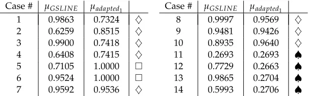
4.1.2 Adapted schemes for all cases of (21) and their rates by LFA

Using the central idea of lagging the small terms in (21) (between 1 and 3 terms), we can derive adapted schemes for all cases in the same manner as for Case 1 previously. In Table 3 we give the comparison of the maximum smoothing rate of GSLINE-I,µGSLI NE, with the maximum smoothing rate of the adapted schemesµadapted1.

The results from Table 3 fall into 3 categories:

♠-cases, where only one term is lagged and the improvements are remarkable. This gives a promising indication that the lagging of particular terms in certain cases can improve the smoothing rate. This motivates our next step.

Case # µGSLI NE µadapted1

1 0.9863 0.7324 ♦

2 0.6259 0.8515 ♦

3 0.9900 0.7418 ♦

4 0.6408 0.7415 ♦

5 0.7105 1.0000

6 0.9524 1.0000

7 0.9592 0.9536 ♦

Case # µGSLI NE µadapted1

8 0.9997 0.9569 ♦

9 0.9481 0.9426 ♦

10 0.8935 0.9640 ♦

11 0.2693 0.2693 ♠

12 0.7729 0.2663 ♠

13 0.9865 0.2704 ♠

14 0.5993 0.2706 ♠

Table 3:Comparison of the maximum amplification factors using GSLINE-I and the adapted iterative schemes for each case. The-cases are the decoupled cases which give a rate of precisely 1, as remarked, the♦-cases have minor or no improvement in the smoothing rate and the♠-cases have a good final rate.

-cases, where 2 terms are lagged and we see the worst results: a smoothing rate of 1.0000 is attained for cases 5, 6 in Table 3. Below we prove analytically that for Case 6 pixels the smoothing rate when using the adapted scheme will always be precisely 1.

Case 6 pixels have the LFA form ˆµi,j=maxα1,α2

|Ai,jeiα1+Bi,je−iα1|

|Si,j−Ci,jeiα2−Di,je−iα2|, and we see a decoupling in the maximisation with respect toα1andα2which allows us to rewrite this as

ˆ

µi,j=

max

α1

Ai,je

iα1_+Bi,je−iα1

min α2

Si,j−Ci,je

iα2_−Di,je−iα2

= max α1

(Ai,j+Bi,j)cos(α1) +i(Ai,j−Bi,j)sin(α1) min α2

Ai,j+Bi,j+Ci,j(1−cos(α2)) +Di,j(1−cos(α2))

+i(Ci,j−Di,j)sin(α2) = r max α1 h A2

i,j+B2i,j+2Ai,jBi,jcos(2α1) i r min α2 h

Ai,j+Bi,j+Ci,j(1−cos(α2)) +Di,j(1−cos(α2)) 2

+ (Ci,j−Di,j)2sin(α2)2

i =

(Ai,j+Bi,j)2

(Ai,j+Bi,j)2

=1,

attained at (α1,α2) = (−π, 0)∈ [−π,π)2\[−π₂,π₂)2. Similarly we have ˆµi,j =1 for Case 5 too.

We claim that it is necessary to have both ofα1andα2in the numerator or denominator of

the LFA formulation to ensure a low smoothing rate. We note that for Cases 5 and 6 this is not the case.

We now focus on improving the♦-cases and the Case 8 in particular and its LFA to motivate us on how to proceed i.e. to see whether an alternative adaptation to the iterative scheme gives a better smoothing rate. The results apply to-cases also.

Improving the adapted scheme for Case 8. A pixel which is labelled as Case 8 is one where

Ai,j,Bi,j,Di,jare relatively small andCi,j is relatively large. Using the previous method we would devise a scheme where the terms with coefficientsAi,j,Bi,j,Di,j would be lagged at time stepkand the term with coefficientCi,jwould be updated to time stepk+1. We pick the particular Case 8 pixel from Table 2 which has the worst smoothing rate and in Figure 2 we look at the smoothing rate for the scheme (15) with different coefficients lagged.

D C D and C B B and D B and C B,C and D A A and D A and C A,C and D A and B A,B and D A,B and C Lagged Coefficients

0 0.2 0.4 0.6 0.8 1

Smoothing Rate

Figure 2:Comparison of the smoothing rate for the Case 8 pixel with the worst smoothing rate when different coefficient terms are lagged. In this case, Ai,j=202,Bi,j=202,Ci,j=137391and Di,j=35(Table 2).

Hence we propose to lag just the smallest of the coefficients in a modified scheme for all cases.

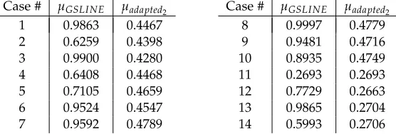
4.1.3 Improved adapted schemes for all cases

We re-consider the♦and-cases which have more than one relatively small coefficient. Lagging only the smallest coefficient, the LFA forms simplify to those of Cases 11–14 and we expect major improvements. In Table 4 we compare the maximum smoothing rate of GSLINE-I,µGSLI NE, for

these cases with the maximum smoothing rate of an improved, adapted iterative scheme which lags only the smallest coefficientµadapted2.

Case # µGSLI NE µadapted2

1 0.9863 0.4467

2 0.6259 0.4398

3 0.9900 0.4280

4 0.6408 0.4468

5 0.7105 0.4659

6 0.9524 0.4547

7 0.9592 0.4789

Case # µGSLI NE µadapted2

8 0.9997 0.4779

9 0.9481 0.4716

10 0.8935 0.4749

11 0.2693 0.2693

12 0.7729 0.2663

13 0.9865 0.2704

14 0.5993 0.2706

Table 4:Comparison of the maximum amplification factors using GSLINE-I and the adapted iterative schemes for each case with just the smallest coefficient term lagged.

As expected, there is a significant improvement in the smoothing rate in all cases when we lag just the smallest coefficient, it also makes implementation faster as we now consider just 4 cases of possible lagged coefficients rather than 14 and therefore have only 4 iterative schemes to consider. Taking our guidance from these results, we propose two hybrid smoothers which both perform standard smoothing iterations on pixels of Ω\D and perform non-standard adapted iterative schemes on the pixels inD.

pixels inD. The potential drawback is that previously updated pixels may enter to the next group of (potentially multiple) updates, making subsequent analysis intractable. Hence our second smoother, denoted by ‘Hybrid Smoother 2’, incorporates partial line smoothing operations at pixels inDand only pixels that are the same line as(i,j)are updated. This line by line approach facilitates subsequent analysis.

4.2.

Hybrid Smoother 1

Our first hybrid smoother updates blocks of pixels at each update, these blocks may overlap. This is an overlapping block smoother of Vanka-type [32, 35]. Once again we start with the setDof pixels with jumping coefficients. For brevity, we will detail the derivation of the iterative scheme for pixels inDfor whichAi,j is smallest. We will then state the schemes for the other laggings (derived in the same manner).

Ai,j lagged. The lagging of coefficientAi,j in equation (15) gives rise to the iterative scheme

Ai,jφ(_i+k)_1,j+Bi,jφ_i(₋k+_1,1_j)+Ci,jφ(_i,k_j+₊₁1)+Di,jφ_i(_,k_j−+₁1)−Si,jφ_i(_,k_j+1)= fi,j, (24)

We are solving forφi−1,j,φi,j+1,φi,j−1andφi,j simultaneously and as we have only one equation, we need three more. We get these by considering (15) at the pixels(i−1,j)and(i,j+1)and

(i,j−1), which gives us the three equations

Bi,jφi,j−Si−1,jφi−1,j= fi−1,j−Bi−1,jφi−2,j−Ci−1,jφi−1,j+1−Di−1,jφi−1,j−1, Ci,jφi,j−Si,j+1φi,j+1= fi,j+1−Ai,j+1φi+1,j+1−Bi,j+1φi−1,j+1−Ci,j+1φi,j+2, Di,jφi,j−Si,j−1φi,j−1= fi,j−1−Ai,j−1φi+1,j−1−Bi,j−1φi−1,j−1−Di,j−1φi,j−2,

which have been rearranged to have theφi−1,j,φi,j+1,φi,j−1andφi,jterms on the left hand side. So, using these along with (24) we obtain the system (25).

Scheme withAi,jlagged:



  

−S_i,j Bi,j Ci,j Di,j Bi,j −Si−1,j 0 0 Ci,j 0 −Si,j+1 0 Di,j 0 0 −Si,j−1

    ·    

φi,j φi−1,j φi,j+1 φi,j−1

    =    

fi,j−Ai,jφi+1,j

fi−1,j−Ci−1,jφi−1,j+1−Di−1,jφi−1,j−1−Bi−1,jφi−2,j fi,j+1−Ai,j+1φi+1,j+1−Bi,j+1φi−1,j+1−Ci,j+1φi,j+2 fi,j−1−Ai,j−1φi+1,j−1−Bi,j−1φi−1,j−1−Di,j−1φi,j−2



  . (25)

This system is strictly diagonally dominant and follows the guidance in [34] that collective update schemes are better for jumping coefficients. This system also has an arrow structure in the matrix and can be solved very quickly (in 24 operations).

4.2.1 The adapted iterative schemes for other cases

Below are the adapted iterative schemes for the cases whenBi,j,Ci,jorDi,j are lagged, derived in the same manner as previously whenAi,j was lagged.

Scheme withBi,j lagged:



  

−S_i,j Ai,j Ci,j Di,j Ai,j −Si+1,j 0 0 Ci,j 0 −Si,j+1 0 Di,j 0 0 −Si,j−1

    ·    

φi,j φi+1,j φi,j+1 φi,j−1

    =    

fi,j−Bi,jφi−1,j

fi+1,j−Ci+1,jφi+1,j+1−Di+1,jφi+1,j−1−Ai+1,jφi+2,j fi,j+1−Ai,j+1φi+1,j+1−Bi,j+1φi−1,j+1−Ci,j+1φi,j+2 fi,j−1−Ai,j−1φi+1,j−1−Bi,j−1φi−1,j−1−Di,j−1φi,j−2



Scheme withCi,jlagged:



  

−S_i,j A_i,j B_i,j D_i,j A_i,j −S_i+1,j 0 0 B_i,j 0 −S_i−1,j 0 D_i,j 0 0 −S_i,j−1

    ·    

φi,j φi+1,j φi−1,j φi,j−1

    =    

f_i,j−C_i,jφi,j+1

f_i+1,j−Ci+1,jφi+1,j+1−Di+1,jφi+1,j−1−Ai+1,jφi+2,j f_i−1,j−Ci−1,jφi−1,j+1−Di−1,jφi−1,j−1−Bi−1,jφi−2,j f_i,j−1−Ai,j−1φi+1,j−1−Bi,j−1φi−1,j−1−Di,j−1φi,j−2



  . (27)

Scheme withDi,jlagged:



  

−S_i,j Ai,j Bi,j Ci,j A_i,j −S_i+1,j 0 0 B_i,j 0 −S_i−1,j 0 C_i,j 0 0 −S_i,j+1

    ·    

φi,j φi+1,j φi−1,j φi,j+1

    =    

fi,j−Di,jφi,j−1

f_i+1,j−Ci+1,jφi+1,j+1−Di+1,jφi+1,j−1−Ai+1,jφi+2,j f_i−1,j−Ci−1,jφi−1,j+1−Di−1,jφi−1,j−1−Bi−1,jφi−2,j f_i,j+1−Ai,j+1φi+1,j+1−Bi,j+1φi−1,j+1−Ci,j+1φi,j+2



  . (28)

4.2.2 Implementing Hybrid Smoother 1

To minimise grid sweeps and ensure that all pixels are covered, we use the following pseudo-algorithm for Hybrid Smoother 2:

I Perform GSLINE-I on all lines in the image.

II For each pixel inD, perform the appropriate scheme of (25)–(28).

We justify the choice of GSLINE-I in stepIas it is the recommended smoothing scheme for a problem with jump coefficients [34]. Note that the schemes inIIcan overlap the same pixels several times due to the collective updates.

Algorithm 2.In future discussion, when we use the Hybrid Smoother 1 in the Full Approximation

Scheme, we will call this Algorithm 2.

4.3.

Hybrid Smoother 2

Our second hybrid smoother first groups pixels inD by whether Ai,j, Bi,j, Ci,j or Di,j are the smallest and then by the line they are on. We then perform partial line updates on these groups for

Ai,j,Bi,j,Ci,jorDi,jin sequence along with individual pixel updates on the other pixels, this avoids the overlap encountered in Hybrid Smoother 1. We note that for pixels inΩ\D the LFA tells us that the smoothing rate is acceptable (maximum 0.7705) and therefore we design a smoother which performs cheap GSLEX-I iterations at the pixels ofΩ\Dand performs the lagged scheme on the other pixels. We focus initially on how we propose implementing this for the pixels inD

with Ai,jlagged and then we generalise the idea to the laggings ofBi,j,Ci,j andDi,j.

Scheme withAi,j lagged. Suppose we focus on a pixel (i,j)∈ Dwhich has coefficient Ai,j the

smallest. If we lag theAi,jthe smoothing rate at this pixel is

ˆ

µi,j= max

(α1,α2)∈[−π,π)2\[−π₂,π₂)2

Ai,jeiα1

Bi,je−iα1+Ci,jeiα2+Di,je−iα2−Si,j

In this new strategy, the only technical issue to address is that, at a pixel (i,j) in set D, the lagged coefficient (hereAi,j) must be a previously updated pixel in this iteration otherwise we cannot avoid multiple updates (as with Hybrid Smoother 1) within one smoothing iteration. Our proposed solution is to view a group of adjacent pixels in setDwhose smallest coefficient isAi,j (shown as starred pixels in Figure 3) and sit on a line as a superpixel and to update together with their Ai,j terms lagged. If the superpixel is comprised of a single pixel, we set its immediate neighbour pixel (here(i,j+1)) as a starred pixel so the group is of size 2. All other pixels in set

D(without smallest coefficient Ai,j) and those not inDare treated as normal pixels (non-starred) and are relaxed by the GSLEX-1 formula. Hence in each smoothing step, starred and non-starred pixels are only updated once.

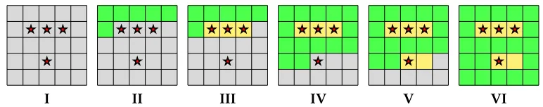
In Figure 3 we illustrate how this proposed algorithm would update the pixels, stepsI–VIrepresent one iteration of the smoother on the 5×5 grid. The starred pixels represent those pixels which haveAi,j the smallest. The algorithm proceeds as follows:

I We identify the pixels inDwhich haveAi,jthe smallest (indicated by a star).

II Perform GSLEX-I on all non-starred pixels.

III Collective partial line update on adjacent starred pixels.

IV Perform GSLEX-I again on all non-starred pixels.

V If a single starred pixel is found, update collectively with the immediate neighbour.

VI Perform GSLEX-I again on all non-starred pixels.

I II III IV V VI

Figure 3:Illustration of the hybrid algorithm for a pixel grid. Each image represents one step of the algorithm, grey cells are yet to be updated. The star pixels are pixels inDwith Ai,jsmallest. Green represents the update by

GSLEX-I and the yellow pixels are the partial line smoothing updates.

4.3.1 The adapted iterative schemes for other cases

We previously focussed on the case for Ai,jbeing lagged and now discuss other components of our iterative scheme to cover the cases ofBi,j,Ci,jand Di,jbeing lagged.

Crucially, to ensure that the scheme agrees with the LFA we must change the direction of update between the schemes for updatingAi,j,Bi,j,Ci,j andDi,j. For example, if we are laggingBi,jpixels we must update from the bottom-right corner to the top-left moving along rows right to left and from the bottom row to the top row. In Figure 4 we show the order in which the pixels should be updated for each lagging.

smoothing rate at each pixel is small because we have ensured that one of the four multiplying factors is small while the other three are no more than 1.

The broad algorithm (I–VI) is the same in these cases as for the case ofAi,jlagged; we identify the pixels which are of that case, perform GSLEX-I on all others and partial line updates on identified pixels.

Hybrid Smoother 2 performs 4 sweeps of the grid, each repeating the aboveI–Vand differing only in update order and assignment of starred pixels. In Figure 4 we display the order in which the pixels and superpixels should be updated for each lagging.

21 16 11 6 1 22 17 12 7 2 23 18 13 8 3 24 19 14 9 4 25 20 15 10 5

Ai,jLagged

5 10 15 20 25 4 9 14 19 24 3 8 13 18 23 2 7 12 17 22 1 6 11 16 21

Bi,j Lagged

5 4 3 2 1 10 9 8 7 6 15 14 13 12 11 20 19 18 17 16 25 24 23 22 21

Ci,jLagged

21 22 23 24 25 16 17 18 19 20 11 12 13 14 15 6 7 8 9 10 1 2 3 4 5

Di,jLagged

Figure 4:Illustration of the hybrid algorithm for a pixel grid. The star pixels are pixels inDwith Ai,jsmallest. Green

represents the update by GSLEX-I and the yellow pixels are the partial line smoothing updates.

4.3.2 Implementing Hybrid Smoother 2

To ensure all laggings are considered, we sweep forAi,j,Bi,j,Ci,jandDi,j in this order, performing steps (I–VI) on each sweep. These schemes are performed on all pixels inD and we see from Table 4 that the maximum smoothing rate overDfalls from 0.9997 to 0.4789. Therefore to reduce high-frequency errors by 90%, with GSLINE-I this would have needed 7675 iterations but with the adapted iterative schemes we need only 4.

To ensure that all cases are considered, we design a hybrid smoother for which one outer iteration includes four sweeps of the image domain. In the first sweep we lag Ai,j, then in the second Bi,j and so on. We note, for example, that in the sweep with Ai,j lagged, then the pixels with coefficientBi,jsmallest have a poor smoothing rate, however on theBi,j sweep the rate is good for these pixels and poor for those where we haveAi,j smallest. However, as the effects compound multiplicatively, after each outer iteration, the smoothing rate at pixels inDis good and forΩ\D

is also good as these have had 4 GSLEX-I iterations.

Adaptive iterative schemes applied to the Spencer-Chen model [33]. We applied Hybrid Smoother 2 to the Spencer-Chen model. In this case using just GSLINE-I we have a maxi-mum smoothing rate of 0.9990 but using the new smoother, the maximaxi-mum smoothing rate falls to 0.5032. Therefore, to reduce errors by 90% we need 4 iterations rather than 2302. This is a further indication that the technique of using the partial line smoothers at the pixels with jumps in the coefficients is a good way to reduce the maximum smoothing rate of the smoother and the idea transfers to other models.

Improved smoothing rates for other images.We now show how the maximum smoothing rate for

Hybrid Smoother 2 is smaller than GSLINE-I for several images with different levels of Gaussian noise. We compare to GSLINE-I as this is the recommended standard smoother for problems with jumping coefficients. We denote the corresponding maximum smoothing rates asµGSLI NE−Iand

µGSHYBRIDrespectively. Results obtained previously are just for the clean image in Figure 1(a). Here we compare the smoothing rates for noisy versions of this image and also of those in Figure 5.

Image µGSLI NE−I µHYBRID

Figure 1(a) + 1% Noise 0.9743 0.4891

Figure 1(a) + 5% Noise 0.9851 0.4815

Problem 1 0.9960 0.4532

Problem 1 + 1% Noise 0.9900 0.4749

Problem 1 + 5% Noise 0.9991 0.4789

Image µGSLI NE−I µHYBRID

Problem 2 0.9999 0.4736

Problem 2 + 1% Noise 0.9988 0.4886

Problem 2 + 5% Noise 0.9934 0.4518

Problem 3 0.9999 0.4829

Problem 3 + 1% Noise 0.9999 0.4863

Problem 3 + 5% Noise 0.9999 0.4841

Table 5:Comparison of the maximum smoothing rates for GSLINE-I and Hybrid Smoother2for various images.

Algorithm 3. In future discussion, we refer to the Full Approximation Scheme using Hybrid

Smoother 2 as Algorithm 3.

5.

N

umerical

E

xperiments

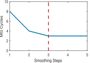
In this section we show two types of numerical experiments: comparisons with the current best methods and analysis of the complexity of Algorithms 2 and 3. Results have been obtained for many artificial and real images but we restrict to the images shown in Figure 5. We show real images as these are of most interest for the application of selective segmentation. The Rada-Chen

Problem 1 Problem 2 Problem 3

and Spencer-Chen models we look at are non-convex and we therefore need the initialisation to be close to the final solution. Thankfully this can be achieved by setting the initial contour as the boundary of the polygon formed from the user selected points inS. For examples of such user defined points, see Figure 7.

Parameter Choices.The values ofc1andc2, being the average intensities inside and outside of the

contour, are updated at the end of each multigrid iteration - the initial values are set to the average inside and outside the initial contour. We fixµ=1/2,λ1=λ2=10−4,ν=1 (for the Rada-Chen

model) andθ=1 (for the Spencer-Chen model). In all experiments we use a V-cycle, i.e. fixγ=1.

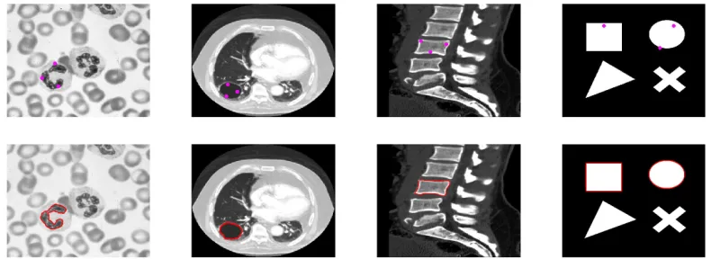
Number of Smoothing Steps.To decide how many smoothing steps were required in Algorithms

1, 2 and 3, we performed experiments to see how the number of smoothing steps impacted the number of multigrid cycles for convergence. As the number of smoothing steps increases, the number of cycles decreases and plateaus. We fix the number of smoothing steps for each algorithm as the number required for the number of multigrid cycles to first plateau. In Figure 6 we demonstrate how the number of multigrid cycles required for convergence changes with the number of smoothing steps and how we choose the optimal number of pre- and post-smoothing steps (ν1andν2). In all tests we use 100 iterations of the exact solver (AOS) on the coarsest level.

Using this technique, we fix the smoothing steps for Algorithms 1, 2 and 3 asν1=ν2=5, 3 and 3

1 2 3 4 5

Smoothing Steps

0 2 4 6 8 10

MG Cycles

Figure 6:The number of smoothing steps plotted against the number of multigrid cycles required to achieve convergence for Algorithm 3 on Problem 1. Guided by this, we choose 3 smoothing steps as the gain plateau’s at this point.

respectively.

5.1.

Comparison of Algorithm 2 and Algorithm 3 with AOS

In this section we compare the speed of the proposed Algorithms 2 and 3 with AOS. We use the image from Problem 1 and scale this to different resolutions. The methods both use the standard

stopping criteria ||φ(k+1)−φ(k)||2

||φ(k)||2 <η, whereηis a small tolerance parameter. In Table 6 we see that Algorithm 3 is faster to reach the stopping criteria (withη=10−4) than Algorithm 2 and that both

due to a higher number of grid sweeps being required in the smoothing steps, however we believe that with improved and optimised coding of the smoother the performance of Algorithm 3 can be increased to achieve far faster convergence than that of Algorithm 2.

Image size Number of Unknowns,N

AOS Algorithm 2 Algorithm 3

Iter CPU Time (s) Iter CPU Time (s) CPU Ratio Iter CPU Time (s) CPU Ratio

256×256 65536 32 3.2 4 3.1 - 4 8.8

-512×512 262144 39 17.3 5 11.6 3.7 3 15.0 1.7

1024×1024 1048576 48 123.5 5 44.0 3.8 3 43.8 2.9

2048×2048 4194304 60 759.2 5 174.2 4.0 3 174.1 4.0

4096×4096 16777216 75 8632.4 5 725.9 4.2 3 688.2 4.0

8192×8192 67108864 * * 5 2952.2 4.1 3 2766.9 4.0

Table 6:For an image of size N=m×n, we show a comparison of the number of iterations and the associated CPU times to achieve the same results for the Rada-Chen model for AOS and Algorithms2and3. ‘*’ indicates that the runtime exceeded 24 hours.

5.2.

Comparison of Algorithms 1, 2 and 3

We now look to see the practical gains from improving the smoother, i.e. the improved smoothing rate of Algorithm 3 should translate into a faster convergence rate [27].

Definition 2. In both Algorithms 2 and 3 we must identify the setD, being pixels at which the coefficients

vary significantly. To do this we compute the minimum multiplicative factor between the largest and smallest of the coefficients Ai,j,Bi,j,Ci,j,Di,j (see §4.1). We will denote the minimum multiplicative factor byΣ.

For completion, we will compare Algorithms 2 and 3 to Algorithm 1 for a range ofΣvalues. The algorithms are all used to segment the image in Figure 1(a), with fine grid 10242and coarse grid 322_andη=10−4_{(all parameters are as earlier in §5).}

Level set energies.In Table 7 we give the energy of the level set at the end of each multigrid cycle

for the Rada-Chen model for Algorithms 1, 2 and 3 for variousΣvalues. The rows are ordered in descending order.

Iteration

1 2 3 4 5 6 7

Algorithm 1 2.4687 1.9333 1.9271 1.9253 1.9247 1.9241 1.9236

Algorithm 2 (Σ=16) 2.4684 1.9333 1.9264 1.9244 1.9238 -

-——–"——– (Σ=8) 2.4683 1.9321 1.9251 1.9242 1.9235 -

-——–"——– (Σ=4) 2.4683 1.9302 1.9242 1.9237 1.9226 -

-——–"——– (Σ=2) 2.4563 1.9269 1.9214 1.9207 1.9199 -

-Algorithm 3 (Σ=16) 2.4300 1.9185 1.9180 - - -

-——–"——– (Σ=8) 2.4253 1.9171 1.9166 - - -

-——–"——– (Σ=4) 2.4184 1.9167 1.9164 - - -

-——–"——– (Σ=2) 2.4136 1.9165 1.9163 - - -

-Table 7:Level set energies (×105) after each multigrid iteration of Algorithms 1, 2 and 3 (for varyingΣ) on the image in Figure 1(a) + 10% Gaussian noise. A dash indicates convergence before iteration number was reached.

and Algorithm 2 gives a lower energy than Algorithm 1 (for allΣvalues). Finally, we notice that asΣgets smaller (and the number of pixels inDincreases), the energy of the level set at each cycle is smaller. This is all in agreement with the theoretical understanding of the smoothers, that they should give a small rate on the pixels inD, and by increasing the size ofDconvergence improves.

Recommended Algorithm.The CPU timings for Algorithm 3 are the best of the three algorithms

(Table 6). The level set energies are also the lowest for Algorithm 3 (Table 7) at each iteration. It performs the best at tackling the PDEs which have many discontinuous coefficients and the experimental results are in agreement with the theory in §4.3. We therefore recommend Algorithm 3 to achieve a fast solution to the Rada-Chen and Spencer-Chen selective segmentation models.

Algorithm 3 Results.In Figure 7 we briefly show the results of Algorithm 3 applied to the test

images for the Rada-Chen model shown in Figure 1(a) and Figure 5 withη=10−4.

Figure 7:Algorithm 3 results; user selections and segmentation results.

5.3.

Complexity of Algorithm 3

We analyse Algorithm 3 to estimate the complexity of each multigrid cycle. We show analytically and experimentally that Algorithm 3 isO(N)as is expected for a multigrid method. We start with analysis of the complexity of the smoother, restriction operator, interpolation operator and coarse grid solver and then use the actual CPU times in Table 6 to confirm the predicted complexity.

Analytical complexity.Consider first only the fine grid with N=nmpixels. Hybrid smoother 2

uses GSLEX-I onKpixels and partial line smoothers on Lsegments, containing the remaining

N−K pixels. GSLEX-I requires 13K operations. The partial line smoothers require O(Mi) operation, whereMiis the size of the line segment fori∈[0,L]. Suppose the number of operations for each partial line smoothing isκMi. We can therefore bound the complexity of the smoothing as 13K+κ∑L_i=0Mi. We know thatK≤ Nand we perform 4 grid sweeps for everyν1pre-smoothing

steps andν2post-smoothing steps. For simplicity, assume a square image (i.e.n=m) and so for

smoothing on one level we have

4(ν1+ν2) 13K+κ

L

∑

Mi

!