Doubly dynamic traffic assignment: simulation modelling framework and experimental results

(1)

White Rose Research Online URL for this paper: http://eprints.whiterose.ac.uk/82752/

Version: Accepted Version

Article:

Balijepalli, NC, Watling, DP and Liu, R (2007) Doubly dynamic traffic assignment: simulation modelling framework and experimental results. Transportation Research Record, 2029. 39 - 48. ISSN 0361-1981

https://doi.org/10.3141/2029-05

[email protected] https://eprints.whiterose.ac.uk/ Reuse

Unless indicated otherwise, fulltext items are protected by copyright with all rights reserved. The copyright exception in section 29 of the Copyright, Designs and Patents Act 1988 allows the making of a single copy solely for the purpose of non-commercial research or private study within the limits of fair dealing. The publisher or other rights-holder may allow further reproduction and re-use of this version - refer to the White Rose Research Online record for this item. Where records identify the publisher as the copyright holder, users can verify any specific terms of use on the publisher’s website.

Takedown

If you consider content in White Rose Research Online to be in breach of UK law, please notify us by

(2)

DOUBLY DYNAMIC TRAFFIC ASSIGNMENT:

SIMULATION MODELLING FRAMEWORK AND

EXPERIMENTAL RESULTS

N.C.Balijepalli#

Institute for Transport Studies 36-40 University Road,

University of Leeds, Leeds LS2 9JT

UK

Tel: +44 (0)113 343 3611 Fax: +44 (0)113 343 5334

[email protected]

D. P. Watling

UK

Tel: +44 (0)113 343 6612 Fax: +44 (0)113 343 5334 [email protected]

R. Liu

UK

Tel: +44 (0)113 343 5338 Fax: +44 (0)113 343 5334

[email protected]

Submission Date: 10 November 2006

Word count: Text - 5147 + 2 Tables – 500 + 9 Figures – 2250 = Total - 7897

#

(3)

ABSTRACT

(4)

INTRODUCTION

Traditionally, dynamic traffic assignment in the literature refers to the modelling of traffic flows on street networks due to the variations in the demand within a day, and capturing the spatio-temporal congestion effects through suitable dynamic link travel time functions. Usually such models are aimed at solving for either dynamic system optimal or dynamic user equilibrium problems. As they consider deterministic flow variables, the solutions naturally tend to be deterministic representing an average situation at each moment. As a result, the within-day deterministic models cannot explain the random variations in traffic flow, besides being unable to represent the transient states in the evolution towards equilibrium (1). In fact, the purview of dynamic traffic assignment is much wider and includes day-to-day variations in the demand in addition to the usual within-day variations. Day-to-day evolution of traffic flows was considered by several authors in the past (1-4), all of whom focused on the evolution of the traffic flows across the days either as a stochastic or a deterministic process, but primarily based on static within-day cost-flow functions. On the contrary, nowadays, more generalised traffic assignment models are being developed which are aimed at addressing both the day-to-day and within-day variations in route flows and such models are called doubly dynamic traffic assignment models, which are the main subject of the present paper.

Cascetta and Cantarella (5) developed such a doubly dynamic simulation model in which they defined the route flows on any day as a stochastic process and included a queuing model to capture the delays on the links. Friesz et al (6) considered deterministic flow variables and defined implicitly a doubly dynamic assignment model considering the day-to-day and within-day dynamics simultaneously, but the model carries with it the usual limitations associated with the deterministic approaches described in the previous paragraph. Balijepalli and Watling (7) developed a variance approximation method to estimate the properties of a stationary probability distribution of a stochastic process in a doubly dynamic environment. Their model was developed as an alternative to the simulation model, based on a deterministic approximation approach. On the other hand, the present paper considers the simulation of route choice process based on a Monte Carlo technique. This paper focuses further on the concept of stationarity of stochastic processes and analyses correlograms as a way of detecting the stationarity based on a necessary condition.

(5)

SIMULATION MODELLING FRAMEWORK

Preliminaries and Modelling Assumptions

Consider a network of directed links serving O-D demand represented by where

is the O-D demand for a particular commodity k, each commodity defining a combination of origin, destination and (discrete) departure period. It is assumed that the total period of analysis is divided into L departure periods. Each commodity k is served by a set of routes with

{

....,q_k,...

=

Q

}

k

q

k

R R_k

elements; the full route set across all commodities thus has dimension

∑

= = K k

k

R 1

ρ . Let f be the

- vector of commodity route flows and c(f) the vector of commodity route costs.

It is assumed that all the trip makers of commodity k are rational in their behaviour when choosing their route, in an attempt to minimise their perceived cost of travel. For each commodity k and route r∈R_k, the perceived travel cost Cˆ_r(n)k at the start of day k is given by

(n)k r 1)k (n r (n)k

r C

Cˆ = − + (1)

where is the population-mean perceived cost for commodity k and route r at the end of

day n-1, and is a random variable describing unobserved attributes contributing to the

population-dispersion of the perceived attractiveness of route r by commodity k. The

k n r

C( −1)

k n r

) ( η

ρ-vector

C(n-1) represents the collection of population-mean perceived costs across all commodities. The probability of choosing route r on day n is then given by:

{

C C

}

i r

Pr ) (

p_rk C(n−1) = _r(n−1)k + _r(n)k < _i(n−1)k + _i(n)k ∀ ≠ (2)

pk(.) then represents the vector (of dimension R_k ) of route choice probabilities for the commodity k, and p(.) denotes the collection of these choice probability vectors over all the commodities so is a vector of dimension . The functional form of the path choice probabilities depends on the joint probability density function assumed for the residuals

{

η_r(n)k :r∈R_k

}

for each commodity k, resulting (for example) in a logit model, if independent Gumbel distributions are assumed, and a probit model for a multivariate normal distribution.

Day-to-day Learning Model

While the behavioural choice-side of the model is quite conventional, a simple linear learning filter is used to replicate drivers building up their experience of travel costs on a day-by-day basis following the completion of each day’s trip. In this research, we assume a simple weighted

average approach akin to many other simulation experiments, for example, Horowitz (9),

(6)

{

( ) ( ) ... ( )

}

)

s( -1 n 1 n 2 m 1 n m

(n)= − + − + + − −

F c F

c F

c

C λ (3)

) 1 /( ) 1 ( )

(

1

1 λ λ

λ

λ =

∑

= − −

=

− m

m

j j

s (4)

where, s( ) is simply a scaling factor to make the weights sum to unity, c(.) the commodity route cost-flow function as defined above, and Fn a vector random variable of dimension denoting the network path flows by commodity on day n.

Stochastic Process Model

The number of drivers in each commodity, as defined by the combination of OD pair and departure period, choose routes independently on day n based on the experienced costs, implying a probability distribution in the space of commodity flows. Assuming that for any day n and for each commodity k, all qk drivers wishing to travel make their travel choices independently conditional on their experiences in the past days, then the number of drivers taking each possible route on day n by each commodity k, conditional on the costs (3) experienced in the past, is obtained as:

(

q , ( ) l

Multinomia

~ k k (n 1)

1) (n

(n)k − −

C p C

F

)

independently for k = 1,2,,….K (5)

where F(n)k is the vector of route flows on day n by the commodity k. The route choice probabilities in equation (5) are computed based on the experienced costs up to the end of the previous day. Individual differences among users in the same commodity are taken into account through random residuals around the population-mean experienced costs defined by equation (3), and hence models of this form are called aggregate memory models. However, in a more general situation, each driver’s perceptions can be modelled through individual learning models, which are called disaggregate memory models, but at the cost of significant computing time (8). It is also noted that OD demand is assumed to be constant, but could be readily extended to the case of uncertain demand as in (11) and ( 12).

Dynamic Network Loading Model

In order to be able to capture the interactions amongst the vehicles departing in the same/successive departure periods, we need to subdivide each departure period into a number of smaller time steps. Let be the time increment of this discretisation, and denote the complete analysis period by (0, N ] for some positive integer N. The time increments are thus the intervals (t- , t] for t = , 2 , …,N , which are referred to as minor time steps. Below, when we refer to a time step (or interval) t, it is to be understood that we are referring to the period (t- , t]. We assume that is chosen so as to be smaller than the free flow time to traverse any link. The OD demand rates are assumed (for notational convenience) to be specified over a common discretisation of the whole analysis period (0,N ], divided it into L major time periods, also

referred to as departure periods (wj-1, wj] (for j = 1,2,..,L) such that

(

w₀,w₁

]

U

(

w₁,w₂

]

U...U

(

w_L₋₁,w_L

]

=

(

0,Nδ

]

. These match exactly the departure periods defined in the previous section, and for convenience are assumed to be of the same duration, i.e.

κ

= − _j₋₁ j w

(7)

Link and Path Travel Times

Assuming that whole link travel time models of linear form (13) are defined on each of the links

on any route r, and that for this route r the links traversed in order are numbered

{

}

the travel time function and exit time functions for any link a

r a a a1, 2,...,

i on this path may be expressed as a nested path cost operator. It is noted that the assumption of linear travel time models is not necessary for the application of our model, as the simulation models can be coupled with any type of link travel time models based on linear or non-linear, continuous or discrete time approaches. However, it is important to note that only the linear travel time function is guaranteed to satisfy the desirable properties such as FIFO (14), and hence has been the choice here. Then the expressions for travel time and the exit time are as given below:

(

g _i₁(t)

)

_i _i

(

g _i₁(t)

)

i a a a a

a − =α +β −

τ

(

i =1,2,...,r; g_a₀(t) ≡ t

)

(6)

(

( )

)

) ( )

(t g ₁ t g ₁ t

ga_i = a_i− +τa_i a_i− (7)

where

()

.

i

a

τ is the travel time on the link ai , αa_ithe free flow time on the link, βai the inverse

of the exit capacity of the link ai, xa_i

()

. the number of vehicles on the link ai , and the exit

time from the link a

(.)

i

a

g

i.

As the model discretises time into a finite number of minor time steps, we have the knowledge of travel times computed only at the discrete time steps. But this will be insufficient to compute the path travel time on any path with multiple links, especially from the second link onwards where the travel time needs to be computed at some real time and not just integers. This is countered by computing the travel time in equation (6) using linear interpolation, which is given below:

(

)

(

)

[

τ δ δ τ δ δ

]

δ δ δ δ

δ τ

τ (t)≈ ˆ (<t/ >. )+t−<t/ >. ˆ (<t/ >+1). − ˆ <t/ >.

i i

i

i a a a

a (8)

for (t ≥ 0; i = 1,2,…,n), where, ˆ

()

.

i

a

τ is the travel time on link ai at integer time, and <t/ > the integer part of time t/ .

Then for example, the path travel time for vehicles entering the link a1 at time t on route r (with ar being the last link on route r before discharging the vehicles to their destination) is simply given as the difference between the exit time from link n and the entry time at the origin, expressed as:

[

g t t

]

t

c( )= _a_r( )− . (9)

(8)

∑

+ − = − ⎪⎭

⎪ ⎬ ⎫ ⎪⎩

⎪ ⎨ ⎧

−

= δ

δ

jn

n j t j j T

r c t

w w c

1 ) 1 ( 1

) ( 1

(10)

where n is the number of minor time steps in major time period T. The departure-time dependent mean travel time obtained from equation (10) is used for updating the drivers’ memorised travel cost in equation (3), which then determines the route choice probability distribution for the following day through (5).

Experimental Set Up

A Monte Carlo simulation method has been used to solve the doubly dynamic assignment problem described. This means that the drivers are allocated to the routes based on pseudo-random numbers generated from a pre-specified distribution with the expected values given by the route choice probabilities. The steps in the simulation are listed below:

[1] initialise the route choice probabilities based on free flow costs (initialisation of (3)); [2] allocate the drivers in various departure periods to routes based on random multinomial experiments (implementation of (5));

[3] compute the departure period dependent experienced route costs based on a dynamic network loading map, (6)-(10);

[4] at the end of day n-1, the population mean experienced route costs are updated using the learning model (3) and the costs fed back to the first step above; and

[5] compute the summaries viz., means, variances and covariances of route flows at the end of the realisation.

EXPERIMENTAL RESULTS

Network Supply and Demand Characteristics

(9)

O1

O2

D1

D2

D3 1

2

3

4

5

6 7

8

9

10

11

[image:9.595.128.484.231.710.2]

12

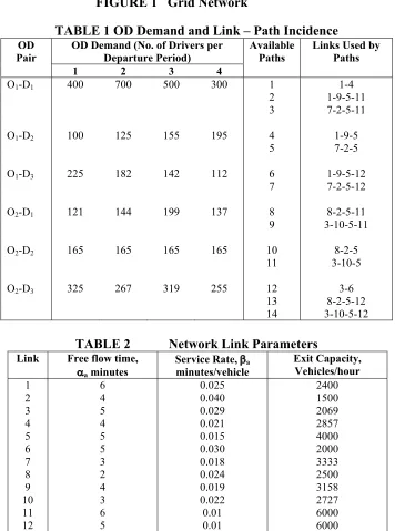
FIGURE 1 Grid Network

TABLE 1 OD Demand and Link – Path Incidence

OD Demand (No. of Drivers per Departure Period) OD

Pair

1 2 3 4

Available Paths

Links Used by Paths

O -D1 1 400 700 500 300 1 1-4

2 1-9-5-11

3 7-2-5-11

O -D1 2 100 125 155 195 4 1-9-5

5 7-2-5

O -D1 3 225 182 142 112 6 1-9-5-12

7 7-2-5-12

O -D2 1 121 144 199 137 8 8-2-5-11

9 3-10-5-11

O -D2 2 165 165 165 165 10 8-2-5

11 3-10-5

O -D2 3 325 267 319 255 12 3-6

13 8-2-5-12

14 3-10-5-12

TABLE 2 Network Link Parameters

Link Free flow time,

αa minutes

Service Rate, βa

minutes/vehicle

Exit Capacity, Vehicles/hour

1 6 0.025 2400

2 4 0.040 1500

3 5 0.029 2069

4 4 0.021 2857

5 5 0.015 4000

6 5 0.030 2000

7 3 0.018 3333

8 2 0.024 2500

9 4 0.019 3158

10 3 0.022 2727

11 6 0.01 6000

(10)

Total Travel Time

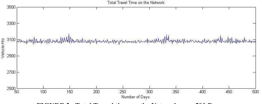
[image:10.595.88.527.177.352.2]

Total travel time measured by the vehicle-hours on the network indicates the intensity of travel over the network, and if monitored over the period of simulation, will indicate the day-to-day evolution of the intensity of travel. Figure 2 shows the day-to-day total travel on the network.

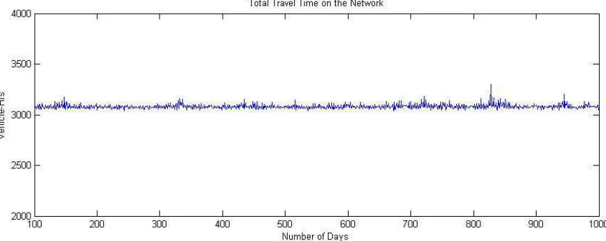
FIGURE 2 Total Travel time on the Network over 500 Days

(11)

[image:11.595.88.525.82.256.2]

FIGURE 3 Total Travel time on the Network over 1000 Days

Stationarity of Stochastic Process

A stochastic process is said to be strictly stationary if its properties remain unaffected by a change of time origin, or in other words, the joint probability distribution of m observations made at any set of times t ( for t = 1,2,..,m) is the same as that associated with m observations separated by an integer k made at set of times t+k (for t = 1,2,..,m and k is an integer) where k is called the lag.

(12)

240 260 280 300 0 0.01 0.02 0.03 0.04 0.05

Mean = 269.20 SD = 9.50

R out e 1 R e lat iv e F req uen c y

Departure Period 1

450 500 550 0 0.005 0.01 0.015 0.02 0.025 0.03 0.035

Mean = 499.88 SD = 13.06

R e lat iv e F req uen c y

Departure Period 2

300 350 400 450 0

0.01 0.02 0.03 0.04

Mean = 367.04 SD = 13.39

Departure Period 3

150 200 250 300 0

0.01 0.02 0.03 0.04

Mean = 228.98 SD = 13.00

Departure Period 4

240 260 280 300 0 0.01 0.02 0.03 0.04 0.05

Mean = 270.26 SD = 9.34

R o ut e 1 R e lat iv e F req uen c y

450 500 550 0

0.01 0.02 0.03 0.04

Mean = 499.51 SD = 14.46

300 350 400 450 0 0.005 0.01 0.015 0.02 0.025 0.03 0.035

Mean = 365.92 SD = 15.73

150 200 250 300 0

0.01 0.02 0.03 0.04

Mean = 227.87 SD = 13.96

Histograms of Route Flows from 201 to 500 days Histograms of Route Flows from 201 to 500 days

[image:12.595.85.529.73.364.2]

Histogramsof Route Flows from 426 to 725 days

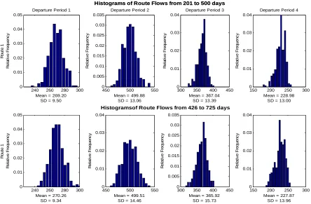
FIGURE 4 Histograms of Flows on Route 1

Visual observation of Figure 4 reveals that the distribution of the flows on route 1 in each departure period is similar in each case for the two sets of the observations. Moreover, in each case the mean and standard deviation of the route flows are nearly identical to each other indicating that the stochastic process being considered is stationary. Histograms of flows on routes 2 and 3 corroborated the earlier comments on route 1 reassuring the stationarity of the process, but due to reasons of brevity they are not included here.

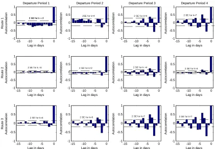
Autocorrelations of Route Flows

(13)

-15 -10 -5 0 -1 -0.5 0 0.5 1

Lag in days

Rou te 1 A ut oc orrel at ion

Departure Period 1

-15 -10 -5 0

-1 -0.5 0 0.5 1

Lag in days

A ut oc orrel at ion

Departure Period 2

-15 -10 -5 0

-1 -0.5 0 0.5 1

Lag in days

Departure Period 3

-15 -10 -5 0

-1 -0.5 0 0.5 1

Lag in days

Departure Period 4

-15 -10 -5 0

-1 -0.5 0 0.5 1

Lag in days

R o ut e 2 Au to c o rr e la ti o n

-15 -10 -5 0

-1 -0.5 0 0.5 1

Lag in days

Au to c o rr e la ti o n

-15 -10 -5 0

-1 -0.5 0 0.5 1

Lag in days

-15 -10 -5 0

-1 -0.5 0 0.5 1

Lag in days

-15 -10 -5 0

-1 -0.5 0 0.5 1

Lag in days

-15 -10 -5 0

-1 -0.5 0 0.5 1

Lag in days

-15 -10 -5 0

-1 -0.5 0 0.5 1

Lag in days

-15 -10 -5 0

-1 -0.5 0 0.5 1

Lag in days

2 SE f or k = 2 2 SE f or k = 2

2 SE f or k =0

2 SE f or k=4

2SE f or k=4

2 SE f or k=2

2 SE f or k=5

2 SE f or k=4

2 SE f or k =4

2 SE f or k=7

2 SE f or k=4

[image:13.595.94.515.72.364.2]

2 SE f or k=7

FIGURE 5 Correlogram for Flows on Routes 1,2 and 3

As the correlation of the flows with themselves is unity, the first bar (with ‘0’ lag) reflects the same. From then on, the autocorrelations can be observed to reduce with increasing lags. Figure 5 includes error bars (based on Bartlett’s formula for large lag standard error (15)) for each of the routes 1,2 and 3, for some lag k>0 beyond which the theoretical autocorrelation function has deemed to have died out. Insignificant autocorrelations compared to standard errors at some lag k>0 indicate that the flows on any route do not depend on the flows on the same route beyond k days during the same departure period. This condition implies that the process is stationary, but it is not sufficient to prove the stationarity. A necessary and sufficient test of stationarity of the time series would be that the determinant of the autocorrelation matrix and all the minors should be greater than zero, thus requiring a large number of conditions to be satisfied, all of which can be brought together by using spectral density functions (15).

(14)

periods contributes substantially to the number of vehicles on the links in periods 3 and 4, resulting in an inflated over-estimation of travel times. This in turn affects the route travel times on any given day, and in turn the route choice of the drivers the following day. Hence, higher autocorrelations in departure periods 3 and 4 are observed than in periods 1 and 2. Had we, on the other hand, adopted travel time functions of a higher order, we would expect the degree of over-estimation of uncongested travel times to be lower, and this may have led to less of a difference in magnitude of autocorrelations between departure periods.

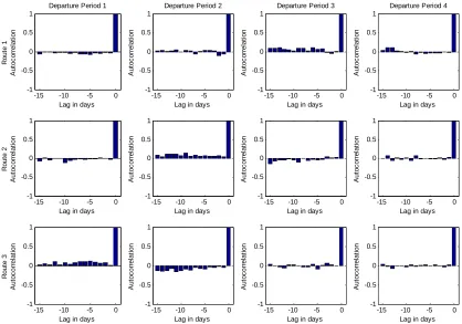
Effect of Varying Perception Error

Quite differently from the above discussion, it is informative to investigate how the autocorrelations reflect a change in dispersion of the perceived costs which is parameterised by the logit choice parameter . As described earlier, autocorrelations in Figure 5 were based on a value of = 0.1. Figure 6 illustrates the autocorrelations of route flows with = 0.01. As decreases (in the limit as θ →0), the dispersion of the perceived costs increases indicating that the drivers ignore the experienced costs and choose routes at random in which case the route flows on any day do not depend on any other day’s flows implying that the autocorrelations will be smaller compared to those in Figure 5. In the limit, the autocorrelations bars will vanish with even lower values of .

-15 -10 -5 0

-1 -0.5 0 0.5 1

Lag in days

Rou te 1 Au to c o rr e la ti o n

Departure Period 1

-15 -10 -5 0

-1 -0.5 0 0.5 1

Lag in days

Departure Period 2

-15 -10 -5 0

-1 -0.5 0 0.5 1

Lag in days

Departure Period 3

-15 -10 -5 0

-1 -0.5 0 0.5 1

Lag in days

Departure Period 4

-15 -10 -5 0

-1 -0.5 0 0.5 1

Lag in days

-15 -10 -5 0

-1 -0.5 0 0.5 1

Lag in days

-15 -10 -5 0

-1 -0.5 0 0.5 1

Lag in days

-15 -10 -5 0

-1 -0.5 0 0.5 1

Lag in days

-15 -10 -5 0

-1 -0.5 0 0.5 1

Lag in days

Ro u te 3 A u to co rr e la ti o n

-15 -10 -5 0

-1 -0.5 0 0.5 1

Lag in days

A u to co rr e la ti o n

-15 -10 -5 0

-1 -0.5 0 0.5 1

Lag in days

-15 -10 -5 0

-1 -0.5 0 0.5 1

Lag in days

[image:14.595.96.514.360.653.2]

(15)

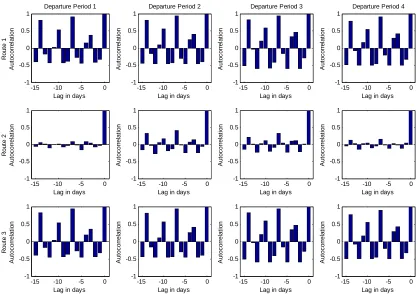
On the other hand, increasing values of will reduce the dispersion of the perceived costs and then the drivers start thinking alike while perceiving the route costs and making route choices. Due to this lack of taste variation, the solutions tend to be ‘all-or-nothing’ in the limit, giving rise to a kind of deterministic periodic system. In this case, most of the drivers choose the least cost route on any given day, then there is very little probability that they choose the same route on the following day, because they experience high cost of travelling on the previous day. This means that the route flows tend to be negatively correlated as shown in Figure 7. In the limit with higher values of , the autocorrelations will be equal to -0.5 at lag k = -1 and -2, indicating a deterministic periodic motion with a period of m = 2. This is true as long as there being another shorter route available to shift to at the end of the day. Otherwise the drivers continue to choose the same route on all days irrespective of the experienced costs (just as in the case of fixed route costs) and then the autocorrelations will be equal to zero for all routes. Due to this reason, in Figure 7, the autocorrelations for route 2 are smaller relative to routes 1 and 2 and are expected to be zero with even higher values of .

-15 -10 -5 0

-1 -0.5 0 0.5 1

Lag in days

Rou te 1 A u to c o rr el at io n

Departure Period 1

-15 -10 -5 0

-1 -0.5 0 0.5 1

Lag in days

A u to c o rr el at io n

Departure Period 2

-15 -10 -5 0

-1 -0.5 0 0.5 1

Lag in days

Departure Period 3

-15 -10 -5 0

-1 -0.5 0 0.5 1

Lag in days

Departure Period 4

-15 -10 -5 0

-1 -0.5 0 0.5 1

Lag in days

-15 -10 -5 0

-1 -0.5 0 0.5 1

Lag in days

-15 -10 -5 0

-1 -0.5 0 0.5 1

Lag in days

-15 -10 -5 0

-1 -0.5 0 0.5 1

Lag in days

-15 -10 -5 0

-1 -0.5 0 0.5 1

Lag in days

-15 -10 -5 0

-1 -0.5 0 0.5 1

Lag in days

-15 -10 -5 0

-1 -0.5 0 0.5 1

Lag in days

-15 -10 -5 0

-1 -0.5 0 0.5 1

Lag in days

[image:15.595.101.519.288.582.2]

FIGURE 7 Correlogram of Flows on Routes 1,2 and 3 ( = 0.5)

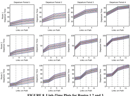
Link Time Plots

(16)

are fanning out in general, meaning that the congestion builds up as we progress with the dynamic loading of vehicles over the network. This phenomenon is particularly clear on links 1 and 2. On the other hand, parallel travel time lines indicate that the links are uncongested and operate below the capacity, as is the case with most of the links on routes 1, 2 and 3. Figure 8 also indicates that the model results are consistent with FIFO property as we do not have any intersecting link travel time lines. The figure is also indicative of satisfying the FIFO property at the path level.

10 4 20

40 60 80

Links on Path

R out e 1 D epa rt ur e T im e

Departure Period 1

10 4 20

40 60 80

Links on Path

D epa rt ur e T im e

Departure Period 2

10 4 20

40 60 80

Links on Path

Departure Period 3

10 4 20

40 60 80

Links on Path

Departure Period 4

10 9 5 11 50

100

Links on Path

R o ut e 2 D epart ur e T im e

1 9 5 110 50

100

Links on Path

D epart ur e T im e

1 9 50 11 50

100

Links on Path

D epart ur e T im e

1 9 5 110 50

100

Links on Path

D epart ur e T im e

7 2 5 110 20

40 60 80 100

Links on Path

R out e 3 D epar tur e T im e

7 2 5 110 20

40 60 80 100

Links on Path

D epar tur e T im e

7 2 5 110 20

40 60 80 100

Links on Path

D epar tur e T im e

7 2 5 110 20

40 60 80 100

Links on Path

[image:16.595.89.519.189.506.2]

D epar tur e T im e

FIGURE 8 Link-Time Plots for Routes 1,2 and 3

(17)

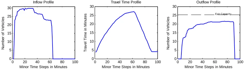
under free flow speeds, the link has still some spare capacity as indicated by the outflow profile lying below the exit capacity.

0 20 40 60 80 100

0 5 10 15 20 25 30

Minor Time Steps in Minutes

N

um

ber

of

V

eh

ic

le

s

Inflow Profile

0 20 40 60 80 100

0 5 10 15 20 25 30

T

rav

el

T

im

e

in M

inu

tes

Travel Time Profile

0 20 40 60 80 100

0 5 10 15 20 25 30

N

um

ber

of

V

eh

ic

le

s

Outflow Profile

[image:17.595.95.520.122.247.2]

Exit Capacity

FIGURE 9 Inflow and Outflow Profiles for Link 2

CONCLUSIONS

The technique of simulation modelling provides solutions to complex traffic assignment problems such as the doubly dynamic traffic assignment described in this paper through a fairly simple and transparent process. For transport modellers applying such models, the practical counterpart to deterministic equilibrium is the stationary state of the stochastic processes, and in this paper correlograms were analysed as a way of detecting the stationarity. Properties of link travel time models including FIFO compliance were illustrated. In the future, affirmative tests of stationarity of the stochastic processes such as the ones involving spectral density functions will be investigated. Further useful experiments could also be performed to investigate the impact of alternative travel time functions (e.g. higher order than linear) on the autocorrelation functions.

ACKNOWLEDGEMENT

The first author gratefully acknowledges the University of Leeds Centenary Chair Research Project for funding this part of the research work.

REFERENCES

(1) Cascetta, E. A Stochastic Process Approach to the Analysis of Temporal Dynamics in

Transportation Networks, Transportation Research B, Vol. 23, No.1, 1989, pp 1-17.

(2) Watling, D.P. Asymmetric Problems and Stochastic Process Models of Traffic

Assignment, Transportation Research B, Vol. 30, No.5, 1996, pp 339-357.

(3) Watling, D.P. and M. Hazelton. The Dynamics and Equilibria of Day-to-day Assignment

Models, Networks and Spatial Economics, Vol.3, No.3, 2003, pp 349-370

(4) Srinivasan, K.K and Z.Guo. Day-to-day Evolution of Network Flows Under Route

Choice Dynamics in Commuter Decisions. In Transportation Research Record: Journal

of the Transportation Research Board, Vol.1894, 2004, pp 198-208.

(5) Cascetta, E. and G.E. Cantarella. A Day-to-day and Within-day Dynamic Stochastic

(18)

(6) Friesz, T.L., D.Bernstein, R.Stough. Dynamic Systems, Variational Inequalities and Control Theoretic Models for Predicting Time-Varying Urban Network Flows,

Transportation Science, Vol.30, No.1, 1996, pp 14-31.

(7) Balijepalli, N.C. and D.P.Watling. ‘Doubly Dynamic Equilibrium Distribution

Approximation Model for Dynamic Traffic Assignment’, in Transportation and Traffic

Theory: Flow, Dynamics and Human Interaction, H.Mahmassani (Ed), Elsevier, Oxford,

UK, 2005 pp 741-760.

(8) Cantarella, G.E. and E.Cascetta Dynamic Processes and Equilibrium in Transportation

Networks: Towards a Unifying Theory, Transportation Science, Vol.29, No.4, 1995, pp 305 -329.

(9) Horowitz, J.L. The Stability of Stochastic Equilibrium in a Two-link Transportation

Network, Transportation Research B, Vol.18, No.1, 1984, pp 13-28.

(10) Nakayama, S., R.Kitamura, and S.Fujii. Driver’s Learning and Network Behaviour:

Dynamic Analysis of the Driver-Network System as a Complex System. In

Transportation Research Record: Journal of the Transportation Research Board,

Vol.1676, 1999, pp 30-36.

(11) Waller, S.T., Schofer, J.L. and Ziliaskopoulos, A.K. Evaluation with Traffic Assignment

Under Demand Uncertainty, In Transportation Research Record: Journal of the

Transportation Research Board, Vol.1771, 2001, pp 69-74.

(12) Sumalee, A., Watling, D. and Nakayama, S. Reliable Network design Problem: The Case

with Uncertain Demand and Total Travel Time Reliability, In Transportation Research

Record: Journal of the Transportation Research Board, (forthcoming).

(13) Friesz, T.L., D.Bernstein, T.E.Smith, R.L.Tobin, and B.W.Wie. A Variational Inequality

Formulation of the Dynamic Network User Equilibrium Problem, Operations Research

Vol.41, No.1, 1993, pp 179-191.

(14) Nie, X. and Zhang, H.M. A Comparative Study of Some Macroscopic Link Models Used

in Dynamic Traffic Assignment, Networks and Spatial Economics, Vol.5, No.1, 2005, pp 89-115.

(15) Box, G.E.P. and G.M.Jenkins Time Series Analysis Forecasting and Control.

Holden-Day, San Francisco, California, 1970.

(16) Astarita, V. A Continuous Time Link Model for Dynamic Network Loading Based on

Travel Time Function. Proc. 13th International Symposium on Traffic and Transportation