This is a repository copy of The design and interpretation of freight stated preference experiments seeking to elicit behavioural valuations of journey attributes. .
White Rose Research Online URL for this paper: http://eprints.whiterose.ac.uk/3390/
Article:
Fowkes, A.S. (2007) The design and interpretation of freight stated preference
experiments seeking to elicit behavioural valuations of journey attributes. Transportation Research B, 41. pp. 966-980. ISSN 0191-2615
https://doi.org/10.1016/j.trb.2007.04.004
[email protected] https://eprints.whiterose.ac.uk/ Reuse
See Attached Takedown
If you consider content in White Rose Research Online to be in breach of UK law, please notify us by
Universities of Leeds, Sheffield and York
http://eprints.whiterose.ac.uk/
Institute of Transport Studies
University of Leeds
This is an author produced version of a paper which appeared in Transportation Research B, and has been uploaded with the permission of the publishers Elsevier. It has been peer reviewed but does not include final publication corrections or paginations.
White Rose Repository URL for this paper: http://eprints.whiterose.ac.uk/3390
Published paper
The design and interpretation of freight stated preference
experiments seeking to elicit behavioural valuations of journey
attributes
Tony Fowkes
Institute for Transport Studies, University of Leeds, Leeds LS2 9JT, UK Tel: ++44 113 343 5340
Fax: ++44 113 343 5334 Email: [email protected]
Abstract
This paper considers how best to establish user valuations of the benefits for freight traffic from reducing both scheduled journey times and the variability of actual journey times. It first looks at who receives these benefits and establishes a case for delving further. A theoretical discussion then shows that estimated ‘values of time’ are likely to be conflations of several different effects, most probably varying from study to study. Results are then given from a case study where special care was taken to separate out these effects. As an Adaptive Stated Preference method is used, arguments are presented that counter the suggestion that resulting estimates will necessarily be biased. The paper ends with some conclusions.
Keywords: Value of Time, Freight, Adaptive Stated Preference, Reliability
1. Introduction
The purpose of this paper is fourfold. Firstly, it is desired to set out a description of what user valuations we may wish to measure, relating to choices between options for moving freight. Secondly, some difficulties in measuring those quantities will be described. Thirdly, results from a case study involving freight movements in the UK will be presented both as an application of some of the points discussed and in order to add to the stock of knowledge in the public domain of the magnitudes of these valuations. Fourthly, the chosen case study survey methodology will be defended in order to enhance confidence in the presented results and begin a discussion of the merits of that methodology.
2. Who benefits from investment in improving journey attributes for freight movements?
2.1. What attributes are of significant interest to freight shippers?
reliability and scheduled journey time. de Jong et al (2004) give a good overview of published results, but not all the presented estimates are directly comparable, for reasons that will be discussed later.
Table1
Order of importance of freight transport attributes (excluding cost) when considering mode choice
Rank
RELIABILITY 1
SCHEDULED TRANSIT TIME 2
FLEXIBILITY (in departure time) 3
CONTROL/TRACKING 4
SECURITY 5
EASE OF (UN)LOADING 6
ENVIRONMENT 7
DAMAGE 8
(EQUIPMENT) AVAILABILITY 9
Source: NERA/MVA/STM/ITS (1997)
Because there are fairly small numbers of freight decision makers and freight movement contracts are usually confidential, it has proved almost impossible to use Revealed Preference to study freight in the UK. Conventional Stated Preference also has its limitations if interviews are required with high level decision makers in big companies. This has led to some use of Adaptive Stated Preference techniques, whereby the design changes within the experiment in reaction to responses (see section 4). Both forms of Stated Preference have to defend themselves against the possibility that respondents will react to a journey improvement as though they were the only one to receive it, and so imagine they will gain a competitive advantage. In the case of a new road scheme, for instance, that will not be the case and so the real value of the improvement may be overestimated.
2.2 What are the benefits to society from reducing freight travel times and their variability?
difficult to unload. Longer and/or less reliable journey times may therefore generate extra costs or diminish the value of the load. For valuable goods, inventory costs may also become important. Fourthly, a longer journey time will dictate either an earlier departure or a later arrival. Both may cause costs by requiring loading staff at inconvenient times. Starting out earlier might rush production and reduce production efficiency. Later arrivals might delay Just-In-Time production processes or lead to stock-outs on shop shelves. To maintain customer service levels a denser network of depots may be required, at greater cost.
The above discussion suggests that the matter of valuing freight travel time and travel time variability may be complex. In addition, there is the obvious link between travel time and its variability such that worries over unreliability can be offset by allowing greater scheduled journey time. This last point will not be considered further, but we will try to understand what journey time related costs there are, and attempt to value them.
3. A theoretical insight
3.1. Introduction
In this section we will attempt to gain insight into how valuations of different disutilities affect the choice of departure time. The sorts of things that need to be taken into account include length of journey time, variability in journey time, cost of departing earlier and the cost of arriving later. Initially, we will temporarily assume that journey time is known (so that the decision on departure time determines arrival time, and there is no journey time variability to consider). This case will be dealt with in a diagram, after which those temporary assumptions will be relaxed in a mathematical treatment incorporating the slopes from that diagram into a Generalised Cost expression together with cost, journey time and journey time variability.
3.2. A helpful diagram
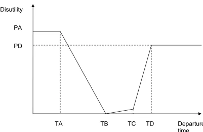
The inability, for whatever reason, to depart at the optimal time, impacts on a business (or supply chain) in various ways. Fig.1 has been drawn on the basis of the following assumptions:
• It is not feasible to depart before time TA (absolutely impossible to have the load ready any earlier, or no vehicle available)
• Time TB is the optimal departure time, against which (dis)utility is measured. Moving from TB towards TA incurs disutility due to rushed production, lorry scheduling difficulties, warehouse staff overtime, etc
• The time (TC-TB) is system slack time, which has a positive utility as it can be used only once
• Beyond TC, penalties arise quickly due to stock-outs, disruption to production schedules, etc
• Beyond TD, it doesn’t matter any more - for whatever reason e.g. the customer has gone elsewhere or the load replaced from another source.
TA TB TC TD PA
PD Disutility
[image:6.595.101.502.82.342.2]Departure time
Fig 1: An illustration of the total disutility (to all parties combined) associated with different departure times, with journey time known and zero variability
3.3. Mathematical treatment
We may summarise what we have just seen in a Generalised Cost (GC) expression:
GC = C + 1JT + 2SP + 3Max(TB-DT,0) + 4Max(DT-TB,0) (1) + 5Max(DT-TC,0) – 3Max(TA-DT,0) – ( 4 + 5)Max(DT-TD,0)
where C is monetary cost,
JT is journey time duration,
SP is journey time spread, reflecting journey time reliability, and DT is departure time
A single binary discrete choice (Revealed or Stated Preference) places the respondent on one side or the other of a Boundary Value Ray (Fowkes, 1991), which delineates attribute valuations that equate the Generalised Costs. In a Stated Preference experiment the Boundary Value Rays can be chosen by the designer, but it may not be possible to isolate the parameter it is wished to estimate. That is the case with equation (1), for example if we seek to estimate the value of 1, as we shall now see.
departure time, with the scheme completed, DT2, will be 5 minutes before TB. For simplicity, let us assume that TA is earlier than DT1.
We have TB-DT1 = 10; TB-DT2 = 5 GC1 = C1 + 1JT1 + 2SP + 10 3 GC2 = C2 + 1JT2 + 2SP + 5 3
Setting GC1=GC2, to find the point of indifference (or Boundary Value) between the two cases, gives:
C1 + 1JT1 + 10 3 = C2 + 1JT2 + 5 3 (2)
Fowkes (1991) defines the Boundary Value of Time (BVOT) to be minus the difference of the costs divided by the difference of the times, ie.
BVOT = -(C1-C2)/(JT1-JT2) (3)
Substituting for (C1-C2) using equation (2), and noting that JT1-JT2=5 gives:
BVOT = ( 1(JT1-JT2)+5 3)/(JT1-JT2) = 1 + 3
Each preference observation places the subject on one side or the other of BVOT, except in the event of indifference between the two cases where we would conclude that
VOT = 1 + 3
We have demonstrated mathematically that estimates of values of journey time ( 1) will be conflated with the value of starting out early ( 3). That may be exactly what we want, but it is useful to understand what is going on. Having an (exogenous) estimate of 3 would allow us to estimate 1, and vice versa. For changes involving time losses it may become necessary to arrive later, in which case other betas come into play.
3.4. Insights gained
deadlines. We may wish to estimate a per-minute disutility arising from these causes. However, we can observe only two times – the departure time and the arrival time. From these two pieces of information it is quite impossible to simultaneously derive estimates for each of these separate three causes of disutility.
For that reason, it is conventional to conflate sources of disutility when deriving values of travel time savings. Theoretical work (following DeSerpa, 1971, and concisely summarised in Mackie, Jara-Diaz and Fowkes, 2001) on the ‘value of time’ defines it to be the sum of the disutility of travel time plus the opportunity cost of that time. In the commuting analogy, that ‘value of time’ would be the value of reducing the difference between the departure and arrival times plus the value of the preferred balance between starting out a bit later and arriving a bit earlier. It is important to realise that the value of a travel time saving (VTTS) is not just the value of reducing time spent travelling, but also includes the benefit gained from leaving later and/or arriving earlier. If we can obtain a separate estimate of the latter we can deduce the former, the extra piece of information giving us the extra degree of freedom we require.
When making decisions on journey times, a range of factors will be taken into account, including those shown in Fig.1 as well as the disutility of having goods in transit and the problems caused by the travel time variability. The preferred outcome will be a trade-off between these various concerns. The diagram shows some fixed constraints as is likely to be the case in practice. Within those constraints there are different penalties/gains for moving departure time backwards or forwards. To counter the uncertainties it is usual to include some slack time in the system as shown in the diagram (TB-TC).
Furthermore, it is to be expected that the true disutility functions will be non-linear, thus the sloped straight lines in the diagram will most likely be curves, possibly sigmoid where appropriate. This suggests that we include non-linear terms in our estimations, and allow for that in our experimental design. However, we are unlikely to be able to have sufficient degrees of freedom to estimate all quantities of interest, so we must prioritise.
4. The Case Study and Leeds Adaptive Stated Preference (LASP) Methodology
4.1. The LASP method
At the time when it became practical to interview respondents in front of a computer it was realised that Stated Preference and Conjoint Analysis designs could be made to react as each response from a given individual was received (see Johnson,1985; and Bradley, 1988). This appeared to offer the prospect of greater efficiency in surveying. This was particularly attractive where the number of potential respondents was small, as can often be the case in studies of freight transport.
various attributes set to particular levels, and asked to rate each alternative. On the next screen, those alternatives liked are generally made less attractive and vice versa. First results were published as Fowkes, Nash and Tweddle (1991). LASP has been used in The Netherlands, Switzerland (Bolis and Maggi, 2002) and India (Shinghal and Fowkes, 2002), besides Great Britain (eg. Fowkes et al, 2004). Danielis and Rotaris (1999) found only 16 studies of freight transport via Stated Preference techniques, of which 5 openly used LASP and a further study used a LASP derived look-alike.
An up to date description of the LASP methodology is given in Fowkes and Shinghal (2002). Once ratings have been obtained for three alternatives over roughly ten choice sets, a transformation is used to yield a logit expression that forms the dependent variable in a weighted linear regression. Bates and Terzis (1992) presented an alternative way of analysing these ratings. Ibáñez and Fowkes (2005) reviewed some alternative ways of modelling LASP ratings.
4.2. The survey
A total of 49 LASP interviews were conducted with transport managers for this study between September 2003 and February 2004, with Non-bulks surveyed first and Bulks later, as part of a larger survey for the UK Strategic Rail Authority. The aim of these interviews was to investigate freight users' willingness to pay for a range of user benefits. The LASP experiment sought to face interviewees with a choice of mode and service quality for a typical flow when given a range of available alternatives provided by a third party carrier at stated costs. Due to limitations on the likely believability/credibility to all respondents of large improvements in service quality, usually alternatives with attributes set at worse than current levels were offered, and the required price discount sought. Only road and rail modes were considered.
Fig.2: Illustration of the LASP iteration screen
The four alternatives were described on the LASP screen in terms of mode (road or rail), latest departure time, earliest arrival time (if there were no delays not specifically allowed for in the schedule), and the time by which 98% of arrivals will have occurred. The LASP screen interpolates 90% and 95% arrival times, for purely presentational purposes. In Column 1, all of these attributes take on their current reported levels. In Columns 2 to 4 one or more of the non-cost attribute levels are varied from those in Column 1, usually such that the service quality is worse. By offering generally worse alternatives, in terms of service quality, than the current service, it is believed that this survey will not be subject to the problem (mentioned in 2.1 above) wherby respondents overstate the benefits to them of a service improvement due to wrongly imagining that they would gain an advantage over their competitors.
distortion to estimates could arise from ‘habit’ effects when the current situation was offered as one of the alternatives in a major study of car drivers’ values of time.
Column 1 remains constant over all iterations. Respondents were asked to rate Columns 2 to 4 on a scale of 1 to 999, where Column 1 is fixed at 100, or to reject a column completely (in which case it was replaced). If advice was sought, respondents were told that if they think one alternative is twice as good as another, then it should receive twice the rating. Once the ratings for the screen were completed, the columns were placed in 'rating order', for the respondent to check that the ranking was as required. If the respondent was happy the ratings (and attribute levels) were recorded and a new screen generated. Subsequent screens react to earlier ratings and attempt to induce respondents to change their rankings of columns (i.e. the ordering of the ratings) and so pass over a Boundary Ray. At some point LASP decides to move on to a subsequent ‘task’ and the process repeats.
4.3. Derived attributes
Table 2: Symbols and Formulae with sample calculation (simplified)
Attribute Formula Journey
1 Journey A Journey B Journey C
Cost (£) 400 300 200 150
Latest Departure Time (G) 18.00 day 1 15.00 day 1 20.00 day 1 20.00 day 1 Earliest Arrival Time
(E) 06.00 day 2 03.00 day 2 08.00 day 2 09.00 day 2
98% Arrival Time (L) 06.30
day 2 08.00 day 2 09.00 day 2 10.00 day 2 J’ny 1 (mins) J’ny A (mins) J’ny B (mins) J’ny C (mins)
Cost Index (C) Indexed to C1 = 200,
C=200£(X)/£(1)
200 150 100 75
Journey Time Duration(JT)
JT = E – G 720 720 720 780
Spread (SP) SP = L – E 30 300 60 60
Early Shift (ESH) ESH = Max (G1–GX–
Max(JTX–JT1 ,0) ,0)
– 180 0 0
Late Shift (LSH) LSH = Max (GX–G1–
Max(JT1–JTX) ,0) ,0)
– 0 120 120
Shift (SH) SH = ESH + LSH – 180 120 120
Lateness (AL) AL = Max (LX–L1 , 0) – 90 150 210
Lateness Squared (ALSQ)
ALSQ = AL2 – 8100 22500 44100
Earliness (AE) AE = Max (G1–GX , 0) – 180 0 0
Earliness Squared (AESQ)
[image:12.595.82.533.110.459.2]AESQ = AE2 – 32400 0 0
Lateness (AL) measures the difference in the offered 98% arrival time from the current 98% arrival time. Journey A illustrates that a journey can still have lateness, even though it has a positive early shift. This is because shift times are only adjusted for changes in journey duration (JT) and not for changes in the length of time between the earliest arrival time and the 98% arrival time, which we call spread (SP). The square of AL is also constructed, ALSQ, for the purpose of capturing a non-linear effect. The counterpart of lateness is Earliness (AE, AESQ).
4.4. The LASP design
LASP can undertake up to 6 tasks, of which 3 are first priority. It was determined that the most important attribute was SP, representing reliability. The two tasks for Column 2 (i.e. one priority and one not) were both allocated to reliability, initially doubling the spread, and then tripling it. By comparing estimates for these two points to the base (Column 1) it was possible to recover a non-linear valuation. The next most important attribute was judged to be journey duration (JT). This was allocated the priority task of Column 3, with latest departure time moved forward by half of JT to give a 50% increase in journey time. The next attribute in order of importance was the “Mode Specific Constant”, or modal penalty for the use of rail. This was allocated the priority task of Column 4, and so that column was labelled “Rail” if the current mode was road (and vice versa). Lastly, there was interest in valuing frequency/flexibility. However, there is little point telling respondents there are two services a day unless they are told when they are. It was deemed appropriate to present the service closest to the current service by moving the latest departure time but holding journey time (and all else) constant. This is achieved by using our time shift attributes (SH, ESH and LSH) to which the remaining two (non-priority) tasks were allocated. Having two tasks so allocated facilitated, in principle, the examination of “earlier” and “later” starts separately, though it was decided that earlier starts were not meaningful for Bulks, for which both tasks were allocated to “later”.
5. Case Study Results
5.1. The Manual method
The first method of analysis used was the Manual method. The Manual modelling looked at all occurrences of a ranking change, involving Column 1, where the non-cost attributes had remained unchanged. For example, if a fall in C (in a particular column) from index 180 (i.e. 180% of the actual current freight rate) to index 160 caused a rating change from 90 to 110, then it would be deduced that the value of that column’s service compared to Column 1 was worth between 20% and 40% of the current freight rate (i.e 180 and 200-160, where 200 is the C for Column 1). The best guess here would be 30%, i.e. halfway between 20 and 40 since 100 (the Column 1 rating) is halfway between 90 and 110. If the only difference between the two columns was that Column 1 was 50 minutes quicker, the value of journey duration (VJT) would be indicated as being 0.6% of the freight rate per minute. Knowing the freight rate allows us to produce monetary estimates. These may then be averaged over groups of firms.
5.2. Weighted regression
The second method, (weighted) regression analysis of logit transforms of the ratios of the ratings, is described in Fowkes and Shinghal (2002). Suffice it here to say that the four columns of the LASP screens were ‘exploded’ to three binary choices, where column 1 was compared in turn to columns 2 to 4. Since we have a continuous dependent variable, the usual techniques of discrete choice modelling are not required. Modelling was conducted for Non-bulks and Bulks separately, models being calibrated for individual respondents. Several model forms were tried. When grouping respondents, it is essential that all respondents in the group have the same model, so the failure of a model to fit for one respondent rules out that model for the whole group. Weightings were chosen on the basis of goodness of fit, with many being tried but just these 3 featuring in the final results: (i) no weight, (ii) the lower of (rate/100)4 or (100/rate)4, (iii) the exponential of the rate divided by the square of one plus the exponential of the rate. The rationale of (ii) was to favour ratings close to 100, while that of (iii) was to accommodate heteroskedasticity.
Again, valuations for groups of respondents may be averaged. In order to minimise the variance of the combined estimate,rˆ, individual valuations, rˆk, are weighted by the inverse of the variance of the estimate, vk, i.e. the valuation which has the greatest variance (i.e. the poorest estimate) gets least weight. Let us denote the variance of the combined estimate by v.
v 1 v rˆ = rˆ k k k
∑
∑
and v 1 1 = v k∑
(4)5.3. Interpreting estimated values
As should be clear from section 3 of this paper, when interpreting model valuations, care must be taken to see which other valuations were derived in the same model. For example, VJT valued scheduled journey time duration, and VAE valued having to start out earlier. If there were an absolute constraint on the arrival time, an increase in the scheduled journey time duration (JT) of x minutes would be accommodated by starting out x minutes earlier. Consequently, it can be deduced that, all else equal, the estimated value of VJT in the absence of VAE in the model would be the sum of the estimated values of VJT and VAE were they both to be present. From the opposite viewpoint, the VJT estimate when both are present has its early start penalty stripped out of it. A second example is the obvious effect on VALSQ depending on whether or not VAL is included.
taken to be the sum of: (i) driver wage savings (DWS); (ii) vehicle operating cost savings (VCS); (iii) the value of journey time reduction (VJT), and (iv) the value of not having to start out so early (VAE). Hence
VTTS = DWS + VCS + VJT + VAE (5)
In line with the insight gained by considering Fig.1, as journey time increases, at some point VAE will be replaced by VAL as an earlier start becomes impractical forcing a later arrival. It should be noted that in this case study VAE has been taken to be zero for Bulks.
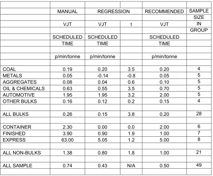
Table 3: Estimates of the value of journey time duration (VJT), expressed in pence per minute per tonne, end-2003 prices
MANUAL REGRESSION RECOMMENDED SAMPLE
SIZE
VJT VJT t VJT IN
GROUP
SCHEDULED SCHEDULED SCHEDULED
TIME TIME TIME
p/min/tonne p/min/tonne p/min/tonne
COAL 0.19 0.20 3.5 0.20 4
METALS 0.05 -0.14 -0.8 0.05 5
AGGREGATES 0.08 0.04 0.6 0.10 5
OIL & CHEMICALS 0.63 0.55 3.5 0.70 5
AUTOMOTIVE 1.95 1.95 3.2 2.00 5
OTHER BULKS 0.16 0.12 0.2 0.15 4
ALL BULKS 0.26 0.15 3.8 0.20 28
CONTAINER 2.30 0.00 0.0 2.00 6
FINISHED 3.90 0.90 1.9 1.00 7
EXPRESS 63.00 5.05 1.2 5.00 8
ALL NON-BULKS 1.38 0.80 1.8 1.00 21
Table 4: Estimates of the value of journey time spread (VSP), expressed in pence per minute per tonne, end-2003 prices
MANUAL REGRESSION RECOMMENDED
VSP VSP t VSP
DELAY DELAY DELAY
SPREAD SPREAD SPREAD
p/min/tonne p/min/tonne p/min/tonne
COAL 0.20 0.19 2.1 0.20
METALS 0.20 0.06 0.4 0.10
AGGREGATES 0.26 0.43 2.1 0.40
OIL & CHEMICALS 0.60 0.78 4.3 0.70
AUTOMOTIVE 2.50 1.06 1.1 2.00
OTHER BULKS 0.43 1.46 1.3 0.80
ALL BULKS 0.98 0.26 4.1 0.40
CONTAINER 5.00 0.50 0.6 3.00
FINISHED 2.90 0.55 2.0 1.00
EXPRESS 22.50 10.70 7.9 10.00
ALL NON-BULKS 8.55 0.95 3.6 2.00
ALL SAMPLE 4.22 0.56 N/A 1.00
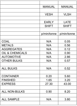
Table 5: Estimates of the value of journey time shift (early (VESH) and late (VLSH)), expressed in pence per minute per tonne, end-2003 prices
MANUAL MANUAL
VESH VLSH
EARLY LATE
SHIFT SHIFT
p/min/tonne p/min/tonne
COAL N/A 0.05
METALS N/A 0.56
AGGREGATES N/A 0.12
OIL & CHEMICALS N/A 0.90
AUTOMOTIVE N/A 2.86
OTHER BULKS N/A 0.57
ALL BULKS N/A 0.52
CONTAINER 0.20 5.60
FINISHED 1.65 3.20
EXPRESS 27.30 43.00
ALL NON-BULKS 0.90 8.20
Table 6: Estimates of the value of early start (VAE) expressed in pence per minute per tonne; and the value of its square (VAESQ), expressed in pence per minute squared per tonne, end-2003 prices
REGRESSION RECOMMENDED REGRESSION RECOMMENDED
VAE t VAE VAESQ t VAESQ
EARLY EARLY EARLY EARLY
START START START SQ START SQ
p/min/tonne p/min/tonne p/minsq/tonne p/minsq/tonne
COAL N/A N/A
METALS N/A N/A
AGGREGATES N/A N/A
OIL & CHEMICALS N/A N/A
AUTOMOTIVE N/A N/A
OTHER BULKS N/A N/A
ALL BULKS N/A N/A
CONTAINER -2.45 -1.3 -1.00 0.00428 1.9 0.00400
FINISHED 0.35 1.1 0.50 0.00061 2.3 0.00060
EXPRESS 4.65 2.2 5.00 0.00022 0.1 0.00020
ALL NON-BULKS 0.40 1.2 0.50 0.00070 2.5 0.00070
Table 7: Estimates of the value of late arrival (VAL) expressed in pence per minute per tonne; and the value of its square (VALSQ), expressed in pence per minute squared per tonne, end-2003 prices
REGRESSION RECOMMENDED REGRESSION RECOMMENDED
VAL t VAL VALSQ t VALSQ
LATE LATE LATE LATE
ARRIVAL ARRIVAL ARRIVAL ARRIVAL
SQ SQ
p/min/tonne p/min/tonne p/minsq/tonne p/minsq/tonne
COAL 0.28 2.2 0.10 0.00011 2.2 0.00005
METALS -0.03 -0.2 0.05 -0.00003 -0.5 0.00002
AGGREGATES 0.26 2.2 0.25 -0.00016 -0.9 -0.00060
OIL & CHEMICALS 0.40 1.8 0.40 0.00000 0 -0.00006
AUTOMOTIVE 1.86 1.9 1.50 0.00019 0.2 0.00004
OTHER BULKS -1.02 -0.5 0.05 -0.02964 -1.9 -0.00006
ALL BULKS 0.20 2.9 0.20 0.00004 1.1 0.00001
CONTAINER 4.55 7.2 4.50 0.00111 2.8 0.00120
FINISHED 1.00 3.8 1.00 0.00008 1.1 0.00000
EXPRESS 11.50 7.6 20.00 0.00661 1.6 0.01000
ALL NON-BULKS 1.80 7.5 1.50 0.00001 1.6 0.00003
ALL SAMPLE 1.00 N/A 0.75 0.00003 N/A 0.00002
5.4. The value of journey time duration (VJT)
Turning to Non-Bulks, high estimates of VJT were obtained from the Manual Analysis. The Regression analysis gave a zero VJT estimate for CONTAINERS, which may be correct when one considers how long some of them are left waiting at ports awaiting collection, but which we ignored in favour of a recommendation (£24/hr/lorry-load) near to the Manual estimate. Strength of feeling regarding that recommendation is not great, and zero would not be unreasonable. FINISHED (ie. General) goods had higher estimated VJT but were given a lower recommended value (£12/hr/lorry-load). Lastly, movements that we classified as EXPRESS, such as parcels operations, had a Regression and recommended estimate of £60/hr/lorry-load.
5.5. Value of Reliability (Spread, VSP)
Estimated values for VSP (Table 4) are generally between the VJT estimates and twice those estimates. Recommended values for VSP for the whole sample, and the Bulks and Non-bulk subgroups are set exactly double those for VJT.
5.6. Early and Late Shifts, Starts and arrivals (VESH, VLSH, VAE, VAESQ, VAL, VALSQ)
Only poor results were obtained from the Regression models for the journey time shift variables, so Table 5 merely reports the Manual analysis results. Bulks were only subject to late shifts. COAL and OIL again yielded sizeable estimates, with those from AUTO much larger. The recommended VLSH for Bulks was around £10/lorry-load for a retiming of one hour later, for a particular shipment. For Non-bulks, estimates of both VESH and VLSH are available. For CONTAINERS, early shift is hardly valued at all, whereas for EXPRESS movements, possibly working on a hub and spoke system and awaiting feeder traffic, it was very highly valued. Values for later retimings were even higher. The recommended values for Non-bulks, for VESH and VLSH respectively, were approximately £11 and £100 per lorry-load per hour.
Tables 6 and 7 report Regression models of the early start (AE) and late arrival (AL) variables. Again, early starts were not possible for the Bulks. For Non-bulks it was intended that the quadratic possibilities would allow for the TA to TB segment in Fig.1 to be curved. Containers actually seemed to favour an earlier start, but non-significantly and there was a positive penalty attached to the square of early start time (AESQ), though the combined effect would only become positive after 10 hours (trimmed to 4 hours recommended). FINISHED (ie General) goods had a small positive VAE, again non-significant, plus a small positive VAESQ. EXPRESS goods have a large significant VAE with a small insignificant VAESQ. The chosen recommended values give a £56 disbenefit per lorry-load for a one hour forced early start.
hand, no late penalty could be found. For AUTO, the penalty for a one hour late arrival would be about £10 per lorry-load. Turning to Non-bulks, FINISHED goods had a similar lateness penalty to AUTO, whilst containers had a penalty of about £50 for a one-hour late arrival. EXPRESS goods were again subject to severe penalties. For being one hour late, the penalty was estimated to be some £140 per lorry-load, rising to £300 when two hours late.
5.7. Conclusions on the Case Study findings.
The presented results are from a small sample in one country at a particular point in time. Nevertheless, they illustrate many of the points discussed in this paper and give some guide as to magnitudes. In practice, as was allowed for in Figure 1, some slack or buffer time will be built into schedules, so a particular lorry faced with the option of using a free congested road or a quick toll road may not actually pay the toll even when the valuations presented in this paper suggest they should. That lorry may have some slack time left and may have little incentive to arrive ‘early’. For many commodities, the value of a scheduled journey time saving (over and above driver’s wages and vehicle operating cost savings) is shown to be relatively small, with the same going for reliability improvements. For some other commodities there does seem to be a significant willingness to pay. Fuller results from the case study are available in Booz Allen Hamilton and ITS Leeds (2004).
6. Are the Results subject to Bias?
6.1 Defence of the LASP method
A major advantage of Adaptive Stated Preference (ASP) in studying freight decision making is that we can hope to obtain much greater information per respondent. Indeed, LASP fits models to each respondent, and then averages over valuations obtained from a group of respondents. In passenger transport studies this is rarely important, as respondents are usually plentiful and reasonably homogeneous. Freight decision makers are much fewer, and much more disparate. In the first LASP study (Fowkes, Nash and Tweddle, 1991) we chose to interview the GB cement industry, at that time comprising 6 companies, of which 4 agreed to be interviewed. We could only have increased our sample size above 4 by including ‘similar’ industries. Besides the problems of expense and exactly how we could define ‘similarity’, we would clearly dilute the ‘cement content’ of our sample. By the time we had a conventional SP sample size we would probably have had to include all bulks.
Whilst these arguments in favour of ASP have generally been held to be persuasive, there have been great concerns that ASP is prone to biases. There are anecdotal reports that some early ASP studies had problems with poor, i.e. implausible, estimates. Bradley and Daly (1993) conducted simulations that -
did not produce accurate estimates due to high correlations introduced between the design variables.”
The theoretical reason why this should be the case was not particularly clear, but allowing the explanatory ‘X’ values (i.e. the attribute level differences) to vary in response to (previous) response ‘Y’ variable (i.e. the respondent’s rating) looked to be far removed from the statistician’s ideal regression theory. The practice of ASP, other than LASP, greatly diminished in subsequent years. Perseverance with LASP was never on the grounds that LASP was not susceptible to bias. It is accepted that analysis of LASP results will be subject to problems arising from endogeneity, but attempts have been made to keep any adverse effects to a manageable scale in the following 3 ways:
(i). Firstly, the model is calibrated at the level of the individual respondent. It is not difficult to see that estimation over several respondents all of whom had been taken off in their own direction by the Adaptive SP could give rise to bias. To give a very stark example, if the number of responses per respondent were variable, and if respondents with high values were asked more questions (say because the experiment started off looking for low values and only slowly adjusted to responses of high value respondents, cutting off only once ‘close enough’) then naively pooling these responses will give a bias towards high values as they are over-represented in the data set. This was not the case simulated by Bradley and Daly, but they were grouping non-homogenous respondents and something similar may have been occurring. LASP models only individual respondents.
(ii). Secondly, LASP has a manual analysis method, which involves looking for indifference, or bounds for the indifference point. For example, a respondent observed to be willing to pay £4 but not £5 for a ten minute time saving might reasonably be taken to have a value of time in the range £24/hour to £30/hour, with the actual ratings allowing a more accurate estimate within that range. It is not easy to see how these manual estimates can be biased to any non-negligible extent. Comparative results for the Manual and Regression methods were presented in Tables 3 and 4, and showed good agreement. Since the Manual results cannot be biased, there cannot be much bias in the Regression model results.
experiment, but they do show that asymptotically the method seems to find the correct value, and there seems little pattern in the errors.
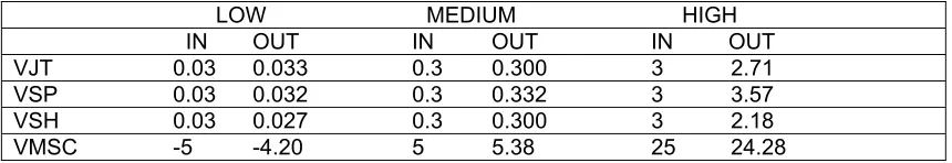
Table 8: Simulation results from 324 combinations of input attribute levels
LOW MEDIUM HIGH
IN OUT IN OUT IN OUT
VJT 0.03 0.033 0.3 0.300 3 2.71
VSP 0.03 0.032 0.3 0.332 3 3.57
VSH 0.03 0.027 0.3 0.300 3 2.18
VMSC -5 -4.20 5 5.38 25 24.28
As can be seen, the simulation results were best for the ‘medium’ values in the middle column, which is as it should be as these were the centre of the attribute valuation space for which the experiment was designed. Despite the extra attention given to the estimation of the reliability variable (VSP), in the ‘Medium’ column its recovery is the poorest. Looking at all three columns, we see that VSP is the only valuation overestimated in all three cases. Of the 12 values simulated, 6 were overestimated, 4 were underestimated, and 2 were spot on. Indeed, if we consider the absolute values, the -4.20 can then be taken as an underestimate, giving 5 of each. These results are not felt to be suggestive of serious bias. Experience with LASP has shown that as the accuracy of an estimate improves (due to alterations to the design), the apparent bias reduces – contrary to the notion of bias as defined by statisticians. It might be reasonable to conclude that LASP is, in some broad sense, asymptotically unbiased.
7. Conclusions
This paper has considered the concepts of freight value of time and reliability, discussed some of the difficulties involved in deriving monetary estimates of them, and provided illustrative results for the UK. It has been stressed that the concept of value of time is vague and situation specific. A road scheme appraisal, for example, will require an estimate of the value to society of a consequential travel time saving. This paper has argued that this VTTS will be the sum of the value of getting the goods to the destination more quickly (VJT), savings in drivers’ wages (DWS), reductions in vehicle costs (VCS), and reduced disutility from being able to make a later start or earlier arrival (VAE, VAL). A related point is that value of time estimates will vary according to the organisation of the freight movement. A company moving goods on ‘Own Account’ will value savings in drivers’ time (and possibly vehicle cost savings) over and above the benefits of journey time savings perceived by shippers using a ‘Third Party’ carrier.
estimated valuation of one attribute sometimes necessarily varied according to the presence or otherwise in the model of a related variable. The main empirical finding from the case study was that, when respondents ignore driver and vehicle costs, for many commodities valuations of improvements in journey time and its variability are negligible, which is in line with current UK Department for Transport thinking. However, shippers of some commodities do exhibit some willingness to pay, occasionally quite a lot. The results presented here may help revise appraisal methods for projects giving time and reliability gains, while the reverse case of increased journey times and unreliability from transport systems running ever closer to capacity can also be valued using these estimates.
The paper ends by defending the Adaptive Stated Preference methodology against worries of bias. It was accepted that there was always a danger of endogeneity bias, but it was argued that good experimental design, checked with simulations, could provide results that showed no significant bias.
Acknowledgments
References
Bates, J. J., 1999. Value of Time on UK Roads 1994: an assessment of the HCG/Accent Report, published in: The Value of Travel Time on UK Roads – 1994, Accent Marketing & Research and Hague Consulting Group, The Hague, 301-324.
Bates, J.J., Terzis, G.,1992. Surveys involving adaptive stated preference techniques. In Westlake, A. et al, (eds.), Survey and Statistical Computing, Elsevier Science Publishers B.V.
Bolis, S., Maggi, R., 2002. Stated preferences – Evidence on shippers’ transport and logistics choice. Chapter VII in Danielis, R., Freight Transport Demand and Stated Preference Experiments. FrancoAngeli, Milan, 203-222.
Booz Allen Hamilton and Institute for Transport Studies, University of Leeds, 2004. Freight User Benefits Study. Final Report for Strategic Rail Authority. Available at
http://www.dft.gov.uk/stellent/groups/dft_railways/documents/page/dft_railways_ 611117.pdf
Bradley, M., 1988. Realism and adaptation in designing hypothetical travel choice concepts. Journal of Transport Economics and Policy 22, 121-137.
Bradley, M., Daly, A. J., 1993. New analysis issues in Stated Preference research. PTRC conference paper, reprinted in Ortuzar, J. de D., (ed.), Stated Preference Modelling Techniques, Perspectives 4. PTRC, London, 2000, 121-136.
Danielis, R., Rotaris, L., 1999. Analysing freight transport demand using stated preference data: a survey, Transport Europei, Anno. V. 13, 30-38.
de Jong, G., Kroes, E., Plasmeijer, R., Sanders, P., Warffemius, P., 2004. The Value of Reliability. Paper presented at ETC 2004, 4-6 October, Strasbourg, France.
DeSerpa, A., 1971, A theory of the economics of time. The Economic Journal, 81, 828-846.
Fowkes, A. S., 1991, Recent developments in stated preference techniques in transport research, PTRC conference Brighton, reprinted in Ortuzar, J. de D., (ed.), Stated Preference Modelling Techniques, Perspectives 4. PTRC, London, 2000, 37-52.
Fowkes, A. S., Nash, C. A., Tweddle, G., 1991. Investigating the market for intermodal freight technologies. Transportation Research Part A 25, 161-172.
Fowkes, A. S., Shinghal, N., 2002. The Leeds Adaptive Stated Preference Methodology. Chapter VI in Danielis, R., Freight Transport Demand and Stated Preference Experiments. FrancoAngeli, Milan, 185-201.
Fowkes, A. S., Tweddle, G., 1988. A computer guided stated preference experiment for freight mode choice. Proceedings of PTRC conference, Bath, published as Transportation Planning Methods, code P306, PTRC, London, 295-305.
Ibáñez, N., Fowkes, A. S., 2005. Factors determining freight transport demand: a comparative study of estimation methodologies. Paper presented to the 37th Annual Conference of the Universities’ Transport Study Group. Bristol (UK) 2005.
Johnson, R. M., 1985. Adaptive conjoint analysis. Sawtooth Software Inc., Idaho.
Mackie, P. J., Jara-Diaz, S., Fowkes, A. S., 2001. The value of travel time savings in evaluation. Transportation Research Part E 37, 91-106.
NERA, MVA, STM, ITS, 1997. The potential for rail freight. A report to the Office of the Rail Regulator. ORR, London.