Intelligent control using generalizing case based reasoning with neural networks

(1)

Reasoning with Neural Networks

Thesis by

David S. Babcock

In

Partial Fulfillment of the Requirements for the Degree of

Doctor of Philosophy

California Institute of Technology Pasadena, California

2000

(2)

(3)

Acknowledgements

(4)

Abstract

One model of human learning involves choosing an action based on past experiences in similar situations. The chosen action is typically modified to compensate for any dis-crepancies with the current situation. After sufficient experience has been obtained,

at least in a particular regime, the experiences are conceptualized into a general response mechanism. This thesis presents an algorithm that formalizes this hybrid reasoning process and applies it to control of a nonlinear physical system. Experiences are stored as vectors of variables known as cases in a set called a casebase. Vector

norms are used to select an appropriate case from the casebase which is then modified

using an adaptation routine. Once the modified action is applied to the system and the resulting outcome is observed, the casebase is augmented to include the new expe-rience for improved future performance. A gated expert neural network is eventually trained on subsets of the casebase to create local inverse model approximations for

regions of the input space where sufficient data is available to support generalization.

The gate network selects one of the experts if appropriate or otherwise defaults back to case-based reasoning. The applicability of the hybrid algorithm is demonstrated

(5)

41

43 43

44

46 46

48 49 49

50

(8)

List of Figures

2.1 Pictorial representation of an artificial threshold neuron computational element. . . . . 8 2.2 Pictorial representation of a radial basis artificial neuron computational

element . . . .

2.3 Schematic diagram of a threshold element feedforward network. 2.4 Schematic diagram of a (discrete) mixture of experts network

architec-2.5 2.6 2.7 3.1 3.2 3.3 4.1

ture . . . .

Schematic diagram of inverse model control. Schematic diagram of forward model control.

Schematic diagram of perturbative model control.

Schematic diagram of the case-based reasoning algorithm ..

Schematic diagram of the hybrid case-based reasoning and gated expert algorithm . . . .

Case-based reasoning example ..

Diagram of the ball and beam system.

8 9

10

15 17 17

20

25 27

28

4.2 Picture of the experimental ball and beam system. . 31 4.3 Graphical representation of input sequence. . . 32

5.1 Hand tuned PD controller full state simulation results. 40 0.2 Hand tuned PD controller noisy simulation results. 40 5.3 Error convergence for the case-based reasoning algorithm. . 41 5.4 Full state simulation results. . . 42

5.5 Absolute error results for a full state simulation run with Vd

= 0.05.

42

5.6 Position only simulation results. . . 43

(9)

5.8 Noisy simulation results using a noise level of 0.005. 5.9 Physical hardware experimental system results.

(10)

Chapter 1 Introduction

Being members of the animal kingdom, we as human beings have certain basic biolog-ical responses built into our makeup. Often they are referred to as instincts or reflexes and they occur involuntarily whenever the external environment triggers them. We have no control over them and often cannot modify those behaviors. In most situa-tions that we encounter, however, we must decide on an appropriate action to take based on the outcome we desire.

One basic learning model simply involves rote memorization of action-result pairs. This type of reasoning is modeled using some type of reference, for example a lookup table or decision tree. The reference dictates the appropriate action to perform to achieve the desired result based on the current state of the system, hence the decision process consists of merely searching the reference. Learning only involves organizing the reference to expedite the searching, i.e., frequently encountered situations are located more quickly. Clearly this form of learning is constrained to tasks where there is only a limited number of discrete results and system states so that generalization is unnecessary. Furthermore, the system must be time invariant so that the same actions will be applicable at any time, i.e., the only relevant decision variables are the current state and the desired result.

(11)

number of examples from which to draw. In so doing, performance can be improved in subsequent situations by basing the decisions on experiences that are more similar to the current situation.

A third method of producing an action is using concepts. The concepts are gen-eralizations derived from extensive experience. Neural networks are often used to model this type of learning by approximating a mathematical function from a given

set of experiences (input-output data pairs). One condition for this type of learning to be successful is the training data set must be sufficient to adequately represent the

underlying function. Furthermore, the network model must be complex enough to approximate the function but not excessively complex to overfit the data.

The contribution of this thesis is to formalize a synthesis of the above decision processes using a hybrid case-based reasoning and neural network algorithm and

apply it to a nonlinear control problem. Case-based reasoning provides an inference

scheme to make reasonable decisions when only a limited amount of information is available. As more experiences are acquired, storage and retrieval of these experiences

becomes an issue. This problem is overcome by training neural networks on subsets of

these experiences reducing the storage and retrieval concerns. Therefore, the hybrid

system utilizes case-based reasoning to generate data sets that are then generalized

using neural networks when appropriate.

In the implementation of the case-based module, experiences arc stored as vectors

of variables known as cases in a set called a caseba8e. Vector norms are used to select

an appropriate case from the case base which is then modified using an adaptation

(12)

(13)

Chapter 2 Background

2.1 Case-based Reasoning

As Riesbeck and Schank [33] describe case-based reasoning, "input a problem, find a relevant old solution, adapt it." Barletta [4] subsequently lists five issues in case-based system development:

*

representation

*

indexing

*

storage and retrieval

*

adaptation

*

learning.

Simply put, given the desired result and the current system state, the algorithm will select an action from a similar prior experience. Unless the desired result and current situation are identical to the prior experience, the selected action may be modified to compensate for these differences. After executing the new action, the al-gorithm observes the actual results and compares these results to what was expected. The errors provide additional experience that can be used in subsequent trials to improve future performance [10]. In this way, the algorithm increases the proficiency of performing a task through repeatedly acquiring more experiences upon which to draw in the decision process.

(14)

Case-based reasoning is typically used in expert systems for planning and di-agnostic tasks, e.g., medical treatment [2, 23] and fault analysis [21]. It has also been successfully applied to robot navigational control. Ram et al. improve reactive robot performance by utilizing case-based reasoning to discretely select and adapt the control parameters [30]. Ram and Santamaria further develop a technique for implementing case-based reasoning in a continuous fashion and also apply it to the task of robot navigation [31].

2.1.1 Mathematical Analysis of 1D Function Approximation

The rational behind case-based reasoning is to develop an algorithm which "learns"

to improve its performance in subsequent trials through the expansion of the set of experiences, i.e., the casebase. This means that as the casebase grows in size, the error

between the predicted outputs based on case modification and the actual resulting outputs should decrease. The following section gives a result to justify this procedure

in the case of a scalar function.

Assume there is an unknown, twice differentiable function Y

f(x)

such that

1f'(X)1 ::; ,.

Let YI =

f(XI)

and

Y2

=

f(X2).

Furthermore, let

Y A(

x)

=

(Y2 -

Yl)

(x - xd

+

YI

=

k

(x - xd

+

YI

X2 -

Xl

which defines the secant line between

(Xl, YI)

and

(X2' Y2)

with slope k, and define a function

E(X)=y-fj

Since

E(X)

is continuous on

[Xl, X2]

and differentiable on

(Xl, X2),

by the Mean Value Theorem from calculus

E(X)

will achieve an extrema either at

E(XI),

E(X2),

or

where

E'(X)

=

O. Since

E(XI)

=

E(X2)

=

0, either

E(X)

=

0 =}

Y

=

fj

over the interval

(15)

Since

E(X:2)

=

r

X2 E'(x)dx

+

E(xd

=

r

E'(x)dx

+

~X

2

E'(x)dx + E(xd

l XI l XI l i ;

applying the boundary conditions and defining the value at the extrema as

fJ

gives

I

i;

lx2

E' ( X ) d.7:

=

-

_

E' (.7: ) dx

=

,/J

XI X

Considering the unknown function

!(J

:)

,

the Mean Value Theorem also states that k

S ,

over the interval (Xl, X2)' Therefore E'(X) = f'(x) - k must satisfy

, - 1 k 1

s

jE'

(x) 1

s

,

+

1 k I· Wi thou t loss of generality, if we assume that the function is increasing in the interval (.1:[, x) with maximal slope,

+

Ikl,

then over the interval

(x, X:2) the maximal magnitude for the slope is , -

Ikl.

Hence we can bound the

magnitude of the extrema by the following two inequalities

Combining these two inequalities gives

I

fJl

s

2,(x - Xd(X2 - x) (:[,2 - Xl)

Since Xl

<

:1:

<

:J:2, the maximum of (x - Xd(X2 - x) occurs where

d _ _ _ _ _ X2

+

.7:)

(16)

Hence

The last equation says that the maximal error is proportional to the size of the input interval. Therefore, the approximation error decreases as the number of input space intervals is increased, i.e., as more cases are generated. Conversely, a maximal input interval size can be computed for a desired error level assuming an upper bound

on the derivative of the underlying function can be approximated.

2.2 Neural Networks

The human brain operates based on a large distributed array of simple computational

elements called neurons. These neurons are interconnected by a network of axon

and dendrites. Information is passed from neuron to neuron through a series of

electrical impulses which travel along the initiating neuron's axon to the various

synaptic junctions with dendrites of receiving neurons. The signals are coded by the

sequential timing of the impulses (frequency) along with loss based on the location

of the synapse in relation to the receiving neuron's soma (amplitude).

2.2.1 Basic Computational Elements

Artificial neural networks attempt to simplistically model the biological system in a

similar fashion using basic interconnected computational elements. One common

ele-ment consists of a soft thresholding function, often the hyperbolic tangent or logistic function. The inputs to the neuron, Xi, are multiplied by weights, Wi, and offset by

a bias, b. The output of the threshold function is then multiplied by a second gain,

(17)

dements produce a soft thresholding of the weighted inputs. Hence the equation for

a hyperbolic tangent artificial neuron is given below with the corresponding picture in Figure 2.1.

y =

W

tanh

(L

WiXi -

b) - B

l

x •

l

x,

:"

Figure 2.1: Pictorial representation of an artificial threshold neuron computational element.

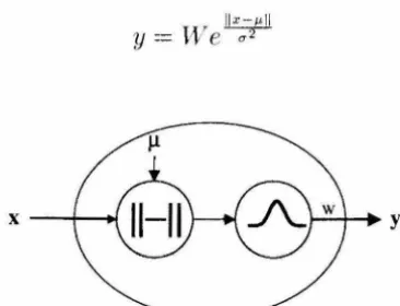
A second commonly used computational element is the radial basis neuron. The

output of this element is a measure of the distance (norm) between the input and the

center (mean) of the basis function. Typically an l2 vector norm is used as the distance

metric and the basis function is some form of gaussian. Such elements produce a

response in a local region of input space around the element's center. In the case of gaussian elements, the degree of localization is controlled by the variance. These

elements are mathematically represented by the following equation and pictorially shown in Figure 2.2.

IIX-/LII Y = J;Ve--;;'l

~+-·Y

Figure 2.2: Pictorial representation of a radial basis artificial neuron computational

[image:17.581.214.391.138.267.2] [image:17.581.210.393.501.641.2]

(18)

2.2.2 Feedforward Networks

To perform useful computations, combinations of the above simple elements are con

-nected in various patterns to form networks. One common connection pattern consists

of organizing the neurons into layers such that the outputs of one layer are fed into

the inputs of subsequent layers. If the connections are only between adjacent layers

with no feedback, the network is called a feedforward network [13] pictorially shown

below in Figure 2.3. Such networks are commonly used with thresholding elements

for model-free function approximation problems.

Wll'

X Y

•

win,

•

Figure 2.3: Schematic diagram of a threshold element feed forward network.

2.2.3 Competitive Networks (Winner-Take-All)

Another type of network, which is often used for input classification problems, is

a competitive or winner-take-all network [13]. These networks consist of uniquely

indexed (usually radial basis) neurons which compute the distance, typically the

Euclidean vector norm, between the input and the neuron's center (mean). The index

of the neuron with the minimum distance, i.e., the "winner," is the output value of the

network. Such networks partition the input space into discrete (perhaps overlapping)

regions. The partitioning is useful when clustering or discrete classification of the

[image:18.579.196.411.245.388.2]

(19)

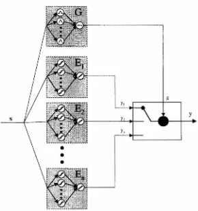
2.2.4 Mixture of Experts Networks

A hybrid network which combines feedforward and competitive networks is known

as a mixture of experts network [34]. This type of network uses several simple

feed-forward networks (experts) whose output is valid for particular regions of the input space (regions of expertise). The input is simultaneously processed by a

competi-tive network (gate) which generates a ranking for each expert. The final output of

the hybrid network is then a combination of the outputs from the experts based on

the gate's rankings. Two common combination techniques involve normalizing the

rankings and applying them as a weighted sum of the experts' outputs (continuous),

or simply selecting the highest ranking expert's output (discrete). The mixture of

experts structure is shown in Figure 2.4.

[image:19.575.152.442.295.603.2]

y x

Figure 2.4: Schematic diagram of a (discrete) mixture of experts network architecture.

These networks avoid the need for a large single network to accurately model input

spaces that are only sparsely populated by locally dense pockets of data. Instead,

(20)

subsets of the data. The gate then only needs to be trained to select the corresponding expert instead of approximate the actual output value. A subsequent advantage of such an architecture is the capacity to add or expand experts to cover new data as it becomes available without retraining the entire network. Only the new expert and the gate networks need to be updated, significantly reducing retraining time.

2.2.5 Learning Models

Backpropagation

An efficient algorithm for training feedforward networks is backpropagation (see [13, 35] for a complete formalization of the algorithm). This method consists of pass-ing the input signals forward through the network to generate the network outputs. These outputs are then compared with the desired outputs to compute an error sig-nal. The weight updates are computed by propagating the error backwards through the network. The backward propagation step is performed using gradient decent to update the weights based on the derivative of the error function with respect to each weight. Weight updates are computed layer by layer since the updates for the (i - 1 )th layer can be computed directly from the updates for the ith layer, hence the

term backpropagation.

Competitive Learning

Training of competitive networks is dependent on the type of problem under

con-sideration. If the output classification is given for the training data, i.e., supervised learning, the network can be trained using backpropagation since the error signal is available. The input space is subsequently partitioned into regions that have pre-defined classifications.

(21)

likelihood metric is the training objective [16]. This procedure involves processing the training examples with the network to produce an initial classification. The mean of the examples in each class is then used to adjust the center of the classifying neuron closer to the mean of the cluster. The network then repeats the reclassification and neuron center updating until a stopping criteria is achieved. This type of learning clusters the data by distributing neurons within densely populated regions of the input space.

Mixture of Experts Training

Since mixture of experts networks are hybrids of both types of networks, both back-propagation and competitive learning are used to train the hybrid network. Initially the gate network (typically a radial basis network) is trained using unsupervised competitive learning. This step separates the training examples into subsets. These

subsets are then used as individual training sets for the expert networks which ap-proximate a local input-output function based on the data. The expert networks (usually standard feedforward networks) are trained using backpropagation. There-fore, the gate network is trained to select the appropriate expert based on the input and then the selected expert is trained to predict the output from the given inputs within its region of expertise.

Perturbative Learning

(22)

2.3 Control Theory

2.3.1 System Identification

The first step in any control design is to model the system to be controlled. This

iden-tification can either be done from physical first principles, empirically from collected

data, or from a combination of both. Such models are inherently incomplete for any

physical system since no model will capture all the dynamics, particularly induced

by noise, of the system. Furthermore, generally the models are linear in nature since

there is a rich set of analysis and design tools available for such systems [19]. If the

system is fairly linear with reasonable noise levels, such a linear model is often

suffi-cient to design a robust controller that achieves the desired performance level when

applied to the real system [8]. However, the model will only be as accurate as the

data used to generate the model. Hence any noise present in either the applied input

signals or in the output sensor measurements will limit the precision to which the

system can be modeled. Furthermore, if aspects of the physical system change over

time, for example due to wear or changes in components, then a new data set must

be obtained to derive a new model.

Model free identification systems, such as neural networks, provide a tool for

generically approximating the input-output map of the underlying physical system (at

least locally) without any a priori knowledge of the dynamics [20, 25]. Such models,

however, generally give no information about the structure of the system, particularly

in operating regimes where no training data is available. Therefore, caution must be

exercised when these models are used for controller design or validation since the

controller may drive the system into regions where the model is not valid. Since the

model can be continuously updated over time as necessary to compensate for changes

in the physical system, however, the controller can simultaneously be adjusted to

(23)

2.3.2 Linear System Analysis

Many powerful techniques for designing robust controllers for linear systems exist [8].

Often times for non-critical applications, a standard PID controller is used. The

controller gains are tuned by hand until acceptable performance is obtained.

Algo-rithms also exist to allow the controllers to be self-tuning where the parameters are

adjusted automatically based on the deviation of the desired output from the actual

output [28]. Such controllers avoid the need for system identification on a

quanti-tative level but have limitations to the systems they are able to adequately control.

More complex systems, either high order linear or nonlinear, require system

identifi-cation before more advanced techniques, such as I-l-synthesis, can be used. Moreover

some systems have nonlinearities, present in any physical system, that are sufficiently

large such that any robust controller designed using linear techniques cannot provide

acceptable performance.

2.3.3 Nonlinear System Analysis

Due to the wide range of possible nonlinear systems, a general controller synthesis

technique does not yet exist. There are techniques which are useful for designing

con-trollers for particular classes of nonlinear systems that satisfy certain conditions [27].

For example, the approximate linearization technique attempts to input-output

lin-earize a system about an operating point and then apply linear control theory to

design a controller [12]. The technique can be repeated for several operating points

and a scheduler implemented to select the appropriate controller depending on the

particular operating point of the system. This technique is effective only if the system

has a significant linear range about the selected operating points. Furthermore, such

a design requires a system identification step for each operating point.

Other techniques exist to design nonlinear controllers that remove the nonlinear

dynamics of the system thus making the extended system linear [15]. The rich set of

linear control techniques can then be applied to the new system to derive a robust

controller. Such procedures again require a fairly accurate system identification,

(24)

2.3.4 Neural

Network

Control

Recently neural networks have been employed in both system identification and

con-troller design [9, 20, 24, 25, 29]. The advantage of neural controllers is their inherent

model-free representation, thus avoiding system identification (although if done may

provide a good initial starting point for training the controller). One disadvantage is

the complexity of the controller must be high enough to model the underlying system

dynamics but not too high that the data is overfit producing poor generalization. Also

the controller must first be trained, either on-line or off-line, before being employed,

which may not be feasible on certain critical or unstable systems. Three neural

con-trol schemes that will be briefly discussed are inverse model control, forward model

control, and perturbative control.

Inverse Model Control

This controller model uses a neural network to approximate the inverse input-output

map of the system [37] and has been applied to many control problems including robot

control [38]. The inputs to the inverse model neural network are the actual outputs

of the system. The desired output of the neural network is the actual applied input

to the system. Hence, the error signal used for training is the difference between the

actual applied input and the input the model network would predict given the actual

system output. A copy of the inverse model network is then used as a feedforward

controller. The desired plant output is input to the controller which then predicts an

appropriate plant input to achieve that output. This scheme is shown in Figure 2.5.

weight copy

[image:24.575.188.404.549.640.2]

(25)

Initially, a rich set of system inputs and resulting outputs needs to be gathered

In order to train a reasonable starting model and corresponding controller. After the initial training, the predicted system inputs from the controller and the resulting

system outputs provide new training examples which are used to continually update

the inverse model and controller. Thus control can be performed successfully even on

systems which change over time (assuming the changes occur on a slower time scale than is required to sufficiently adapt the network). Furthermore, the general function

approximation capabilities of neural networks allow this technique to be applied to both linear and nonlinear systems. One limitation of this technique, however, is that it cannot be used for systems which either do not have an inverse or with an unstable

inverse, since the network will be unable to converge to a stable set of weights.

Forward Model Control

To avoid the problem of the existence of an inverse plant, a second neural control

scheme, known as forward model control, can be used [24, pages 216-217]. This setup

employs two distinct networks, one for the model and one for the controller. The

in-put to the model network is the actual input to the plant (which is also the output of

the controller network). The desired output of the model network is the co rrespond-ing output from the plant. The error signal is the discrepancy between the predicted

output from the model and the actual output. This error signal is backpropagated

through the forward model to update the model weights. Then further bac

kpropaga-tion from the model is applied to update the controller weights. Figure 2.6 shows a

schematic representation of this setup.

Both networks are trained as if they are a single larger multi-layer network. Prac

-tically, two networks are typically used so that they can be updated at different rates, for example updating the weights of the model more frequently than those of the

controller. The advantage of this technique is that the forward model can always be

trained to provide at least a locally accurate model of the plant, hence a local co

n-troller can theoretically also be trained. The disadvantage is that since both networks

(26)

controller weight update

model weight update

[image:26.577.187.402.53.184.2] [image:26.577.191.407.478.577.2]

y

Figure 2.6: Schematic diagram of forward model control.

particularly initially. Hence, if the system is rapidly changing, the networks (the

forward model in particular) may never converge adequately.

Perturbative Control

A third neural control technique involves using only a controller network. The

net-work is trained using perturbative methods [1] where the applied perturbations are

influenced by the performance of the controller. Clearly this technique is of limited

utility due to the slower convergence rates of perturbative learning. However, for

cer-tain systems that have very slow dynamics, such a technique provides for a physically

implement able controller due to the simplicity of the learning algorithm. This simple

scheme is shown in Figure 2.7.

+ on troller weight _update

(27)

2.4 Related Work

Many hybrid schemes have been developed combining case-based reasoning with neu-ral networks and other techniques in various applications. Neural networks have been

combined with case-based reasoning in the medical field for congenital heart disease diagnosis [32J. The hybrid system attempts to circumvent the deficiencies inherent in the two approaches when implemented separately, namely storage and retrieval issues for case-based reasoning and output explanation and interpretation for neural networks. Another hybrid algorithm has been successfully implemented for the design of mixing systems where fuzzy logic and neural networks are used to perform case

adaptation [18J.

Many hybrid schemes have also been implemented in control applications. A combination of a rule-based expert system with fuzzy logic and neural networks was

applied to the truck and trailer backer-upper control problem [14]. Associative

mem-ories, a technique similar to case-based reasoning, has also proven useful for control problems [11]. For example, Atkeson et al. have successfully applied this approach to

train a robot to perform a juggling task [3].

A wide range of controllers have been designed for the ball and beam problem. Hauser, et al. design a nonlinear controller by approximating the ball and beam system with one that is input-output linearizable [12]. Several different variations of fuzzy logic controllers have likewise been successfully applied to ball and beam control [6, 22, 36]. A recurrent neural network solution has been developed by Chu, et al. [7] Finally, Ng and Trivedi present a hybrid fuzzy logic and neural network controller

(28)

Chapter 3 Hybrid Reasoning System

The motivation behind this thesis is to combine case-based reasoning with neural networks to realize the advantages of both methods. Case-based reasoning is used to intelligently generate an initial set of data (the casebase). This data set is then partitioned into local clusters using a radial basis competitive learning network (the

gate). Separate simple threshold neuron feedforward networks (the experts) are then trained to approximate the underlying local input-output functions represented by the local subsets of cases. Whenever the desired output lies sufficiently close to the center of one of the experts, the gate will select that expert to generate the predicted input. Otherwise if no expert is close, the gate will pass the decision to the case-based reasoning module to determine the action to implement. As more cases are generated, the system can retrain or add new experts (and concurrently modify the gate) to incorporate the new information. Furthermore, if the experts no longer produce acceptable results, for example due to changes in the underlying system, they can be removed until a new set of cases is created in that region of input space.

3.1 Case-based Reasoning Model

(29)

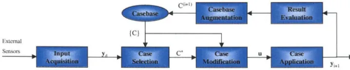
ex-ternal system. The resulting output is analyzed by the result evaluation module to determine whether some type of unusual or anomalous event occurred during the execution of the input. If the output is reasonable, the casebase is expanded using

case augmentation to construct a new experience based on the applied input/resulting

output pair allowing the system to learn from the experience. The entire procedure is shown schematically in Figure 3.1. The remainder of this section describes each of these routines in more detail.

External

[image:29.579.116.475.208.280.2]

Sensors

Figure 3.1: Schematic diagram of the case-based reasoning algorithm.

3.1.1 Case Structure

Each case consists of a number of variables which contain information about the resulting output (and usually the initial state) and the applied input. Hence, a case

is generically defined as a vector C consisting of two subvectors y and

u

c

= [ :

1

where y contains the initial and final states of the system, i.e., the resulting output,

and u contains the applied input. Other values, such as time for execution or expended

energy, may also be included for use in case selection.

3.1.2 Input Acquisition

The starting point of any reasoning system involves acquiring data describing the current state of the system. Human beings use their five senses to collect information

about the environment in which they are operating. Machine systems obtain this

(30)

data can be noisy and cluttered with extraneous information. Hence some form of signal preprocessing, i.e., a filter, is applied so that only the important information is passed on. This preprocessing step is important in improving the efficiency of the

reasoning engine.

For any algorithm to work, the input data must sufficiently describe the current

state of the system. Additionally, the algorithm must also be provided with the

desired result to be obtained. Compiling these two pieces of information in the desired

result vector, Y d, a decision can be made as to what action is necessary to achieve

the desired result given the current state.

3.1.3 Case Selection

Once the desired result vector is constructed, the second step in the reasoning process involves selecting the basis case, denoted by C*, which represents the past experience

that is most similar to the current situation. This selection is done by choosing a

distance metric (typically the l2 vector norm) as a measure of the distance between

the desired result vector, Yd, and the output vector from each case, y(i). A weighting

matrix,

rv

,

can be used to bias the metric in favor of certain important components

within the output vector. Assuming discretely numbered sequential cases indexed by

i, the selection criteria is given by

A useful extension is often to apply a temporal weighting factor to the metric so

that the most recently generated cases are favored more heavily. This technique allows

for the casebase to dynamically adapt to a system that may be changing over time,

for example due to mechanical wear. Since the recent cases represent examples of the

input-output map at the current time, they may be more appropriate for determining

a proper action than distant past experiences, even if the more recent output vector

(31)

Sometimes due to natural symmetry within the system, additional cases can be inferred from the existing ones. In particular, if the system is time invariant, then an

"inverse" case can be created by applying the inputs backwards in time and reversing

the initial and final states.

3.1.4 Case Modification

The input vector from the basis case provides the initial input "guess" denoted by u*.

In general, however, the selected basis case will not be an exact match to the desired result vector. Hence, the system can either directly apply the basis case (u = u*)

thus accepting that significant error may exist in the output, or modify the input

vector from the basis case in an attempt to produce a better output. A common

method of modifying the basis case is to use first order gradient information within a local neighborhood. By numerically approximating the gradient using cases close

to the basis case, a first order linear correction factor can be computed. Depending

on the dimensionality of the system and the density of the cases within the local

neighborhood, higher order corrections can also be computed.

3.1.5 Case Application

After modification of the inputs from the basis case, the final input,

u,

is then applied to the system. The algorithm monitors the state of the system to watch for anomalous behavior. Once the input sequence has completed, the resulting outputs are measured

and passed on to the result evaluation routine.

3.1.6 Result Evaluation

Before constructing a new case, the results must be validated to avoid corrupting the

casebase. The validation step often checks if something anomalous occurred during

(32)

inputs. However, t.he anomalous cases are often stored in a separate casebase so

that modified cases can be compared with them in order to prevent the system from

performing a similar mistake.

3.1. 7

Casebase Augmentation

Assuming nothing anomalous occurred during the execution of the case, the initial

state and resulting output is stored in a vector y(i+I). Combining this vector with

the applied input vector, il, a new case is constructed as

[

(i+I)

1

C(i+I) = Y il

The case base is augmented with this new case which is then used in subsequent case

selection and modification steps.

3.2 Neural Network Generalization

Since each case in the casebase represents an input-output pair from the underlying

system's transfer function, a natural extension is to generalize a sufficiently dense

case-base into a mathematical function. This procedure reduces the storage and retrieval

requirements of the case-based algorithm by directly computing the appropriate

sys-tem input given the desired output. Any function approximation technique can be

employed to generalize the data. For specific systems, it may be beneficial to tailor

the functional form in order to take advantage of physical principles or other known

relationships inherent in the underlying system. Otherwise, model-free

approxima-tion techniques, such as neural networks, can be used for more generic generalization.

Typically these techniques will require more data to avoid overfitting and insure good

generalization performance. The benefit is that they are not restricted to any

(33)

As discussed in Section 2.2.4, mixture of experts networks are often used for problems that have clusters of data. The advantage of this technique is that several simple networks can be quickly trained to cover the important regions of the state space rather than attempting to cover the entire state space with a single complex network. Expert networks are only created in regions where enough experience has been gained to support generalization. Outside these regions, the computed output can either be an interpolated value between experts or an extrapolated one based on the nearest expert. Each expert can be viewed as implementing a local version of inverse model control (refer to Section 2.3.4) and updated whenever it is selected to

generate the system output.

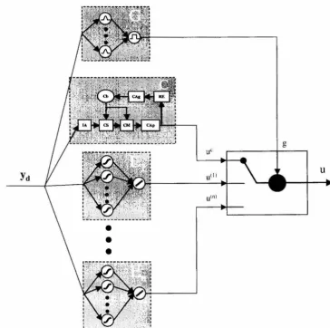
3.3 Hybrid Algorithm

The purpose of this work is to combine a discrete variation of the mixture of experts technique, known as a gated expert network, with case-based reasoning. In this implementation, the gate network produces a winner-take-all decision rather than a vector of mixing coefficients. Hence, each data point is allocated to one and only one

expert, dividing the input space into mutually exclusive regions. The center of each

region, i.e., the mean of the corresponding gate network neuron, is denoted by p,. The algorithm used in this work additionally bounds the regions of expertise of the expert networks to a local area where there is data by setting a threshold, denoted by

f, around the expert centers. This bounding allows the gate to default the decision to the case-based reasoning module if the desired result is not within the regions of expertise of any of the expert networks. Formally the output of the hybrid algorithm

is given by

{ UC u=

u(il minllYd - p,(illl otherwise

z

(34)

A schematic diagram of the hybrid algorithm is given below in Figure 3.2.

g

u"

u

U(II

Figure 3.2: Schematic diagram of the hybrid case-based reasoning and gated expert

algorithm.

3.4 ID Case-based Reasoning Example

The case-based reasoning procedure will now be demonstrated through a simple 1D function approximation problem. Assume the underlying function is given by

f (u)

= eU

over the interval 0 ::; u ::; 1. Furthermore, take as initial cases the four data points

given by

c

=

[

y ]

=

{ [

1.26 ] , [ 1.63] , [ 1.84] , [

2 .

5~

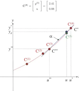
] } u 0.23 0.49 0.61 0.90

[image:34.576.111.475.77.439.2]

(35)

3.4.1 Input Acquisition

For this simple example, the desired result vector is only the desired output value

Yd = 2.44.

3.4.2 Case Selection

L~sing the ahsolute difference as the metric, the distances are computed as follows

IIYd - y(i)

II

=

IYd -

y(i)1

=

{1.18, 0.81, 0.60, 0.15}

Hence, the selected basis case is

C*

=

{C(i)

I

min IIYd - y(i)

II}

=

c(4)

1

3.4.3 Case Modification

In this 10 example, simple first-order linear interpolation will be used to modify 11,*,

refer to Figure 3.3. The nearest case in input space to C*, which shall be denoted by C**, is clearly C(3). Formally,

Therefore, a correction factor, a, is computed as

Yd - y* 2.44 - 2.59

n

=

0.20

y** - y* 1.84 - 2.59

Applying this correction factor gives a predicted input of

(36)

3.4.4 Case Application

Applying the predicted input

u

= 0.88 produces the actual output y =

f(u)

= 2.41

giving an error of

Iy -

Ydl

=

12.41 - 2.441

=

0.03.

3.4.5 Result Evaluation

Since the predicted input is within the interval for which the underlying function is

defined, the output is valid. Therefore, y(5) = 2.41.

3.4.6 Casebase Augmentation

Hence, the case base can be updated to include the new case

C(5) = [ y(5)

1 [

2.41

1

u 0.88

y

*

y

---

- -

--y

d --- ,

ex

,

//

td)

C

*

C(3) ,/ ,/

,/

*

y

---

---C (1) / / / /

.

,-,-,-... '

,-... .,. ... , ...

---+---~**---~~-*~u

[image:36.576.136.454.307.675.2]

u

(37)

Chapter 4 Experimental Setup

4.1 Descript

i

o

n

of Experimental Systems

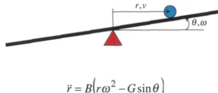
The experimental system selected to demonstrate the hybrid algorithm is the standard

ball and beam control problem [12]. The objective of the control is to rotate the

beam in such a way that the ball position follows a desired trajectory. For the

experiments, three distinct setpoints are defined along the beam and the control

algorithm produces inputs that transition the ball position between these setpoints,

i.e., a setpoint regulation task. The system with corresponding variables is pictorially

given below in Figure 4.1.

-

.

)

8.W

[image:37.584.187.405.346.439.2]

-r

=

B(rm

2 -Gsin8)

Figure 4.1: Diagram of the ball and beam system.

4.1.1 M

athe

matical

Equations for the Sy

stem

Given the moment of inertia for the beam Jb; the mass, radius, and moment of

inertia of the ball

M,

R,

and J respectively; and the acceleration due to gravity G;

the equations of motion for the system are given by

o

=

(~~

+

M)

r

+

MGsinB -

MriP

(38)

where T is the ball position, () is the beam angle, and T is the applied torque on the

beam. Furthermore, setting the input u = () gives

T =

2MTiiJ

+

MGrcos{)

+

(Mr2

+

J

+

J

b) U

Defining a constant

B

as

M

B

= 0

-1&+M

the equations of motion can be rewritten in state-space form as

Xl

.T2

X3

:£4

y

where

X2

B(

x

\

:

d

-

G sin X3)

X4

U

Xl

r

T

X=

()

y=T

However, for the experimental systems under consideration, only the desired beam

angle, X3, can be commanded. Thus the actual dynamics of the beam servo in

(39)

4.1.2 Simulated Systems

The computer simulation computes the dynamics of the equations given above using a fourth order Runge-Kutta method. Constraints are placed on the ball position to account for the ball reaching the end of the beam. If this situation occurs, the ball position is clipped to the beam end and the velocity is set to zero (simulating a stop at each end of the beam). Furthermore, the beam transition dynamics are modeled using a constant angular velocity resulting in a linear angular change from the current

angle to the commanded angle. The program is written such that the simulation runs in real-time with the update time user definable. This setup allows for accurate prediction of the performance of the hybrid control algorithm when applied to the physical system.

The computer simulation allows for three different simulation modes. The first

mode is a full state mode in which the reasoning algorithm is provided with the exact position and velocity of the ball at each update time. The second mode is a position

only mode where the algorithm is given just the exact ball position. In this mode, the controller must approximate the ball velocity thus introducing a time lag into

the velocity measurement. The final mode is a noisy position mode which introduces additive, uniformly distributed noise into each ball position measurement. The noise level is set to roughly correspond with the noise level present in the physical system. For this mode the algorithm is again required to approximate the velocity from the

noisy position measurements.

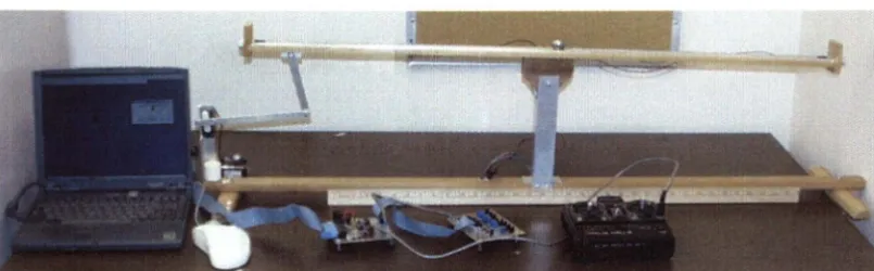
4.1.3 Physical System Construction

The physical system consists of a beam that is 4 ft. in length and utilizes a steel

pinball. The beam is constructed from two parallel rods attached via a mechanical linkage to a standard RC servo. A PC is connected to the system using a custom built

I/O board which attaches through the parallel port. The board consists of buffered analog inputs that are converted to discrete lO-bit integers using a Maxim 186 A/D chip. The board also provides analog output channels with lO-bit resolution using a

(40)

One of the beam's rods is constructed of threaded nylon wrapped with resistive

Ni-chrome wire giving an end to end resistance of approximately 100 ohms. The

second rod is made of aluminum. A fixed voltage from the I/O board (5V) is applied

to the ends of the resistive rod. The ball then acts as a contact between the resistive

wire and the aluminum rod. Hence, the ball's position on the beam is sensed as the

voltage on the aluminum rod. This signal is passed through a simple low pass filter in

order to smooth out the signal before being fed into one of the analog input channels

on the I/O board.

The beam angle is set using an analog output channel on the I/O board. The

analog voltage is fed into a standard RC transmitter which performs the necessary

signal conversion and transmission to a standard RC receiver attached to the beam

support. A servo is then connected to the receiver and mechanically linked to the

beam. This setup provides a generic interface for the computer to control any system

utilizing RC servos. A photograph of the complete system is shown below in Figure

4.2.

[image:40.578.107.510.427.552.2]

(41)

4.2 Case-based Reasoning System

The details of the implemented case-based control algorithm using the structure

pre-sented in chapter three will now be prepre-sented.

4.

2 .1

Case Structu

r

e Variables

The input sequence consists of tilting the beam to a particular angle, Ul, until the

ball passes a particular reference position on the beam, Ym. The beam is then tilted

to another angle, U2, until the ball achieves a particular velocity, _{Vm ,}at which point

the beam is returned to level. This sequence produces a corresponding roughly linear

velocity change and subsequent quadratic positional change in ball position as shown

in Figure 4.3.

e

• t

y",

[image:41.573.222.367.310.544.2]

Yo -1--"'--- - - .

Figure 4.3: Graphical representation of input sequence.

The input sequence variables are stored in a vector, u, defined as

Ul

Ym

U =

U2

(42)

The initial state variables of the system and the resulting output variables are stored

in a vector, y, defined as

b.y

YI - Yo

.6. V VI - Vo

y=

Yo Yo

710 Vo

Combining the above two vectors, the ith case is defined as a vector C(i) as follows

y(i)

C(i) = u(i) .6.t(i)

where .6.t = t I -

to

is the total case execution time.

4.2.2 Input Acquisition Procedure

The reasoning algorithm is given the measured (possibly noisy) ball position, Yo·

For the full state simulations, the algorithm is also given the measured velocity, vo,

otherwise the velocity is approximated by a simple linear regression fit within a sliding

window of positional data. The desired final setpoint, Yd, and desired final velocity,

Vd, are also provided. Thus the desired result vector is constructed as

Yd - Yo

Yd =

Yo

Vo

4.2.3 Case Selection

Procedure

Case selection is based on a weighted 12 norm for both the actual case and the inverse

(43)

1 0

o o

o

0.5 0 0

W=

o

0 0.5 0

o

0 0 0.1

This matrix emphasizes the positional change variable and to a lesser extent the

velocity change and initial position variables. Hence, the basis case, C*, is found by

4.2.4 Case Modification Procedure

Case modification is performed using a simple linear interpolation/extrapolation rou-tine. The casebase is searched to find the adaptation case, C**, that has minimum

distance in input space (again using the l2 norm) from the basis case, C*, selected in the previous step.

A linear correction factor, a, is then computed using the positional change variable as

6.Yd - 6.y* a = -6.y** - 6.y*

The correction factor is used to compute the actual input, u, to be applied to the beam as follows

(44)

Additionally, the transition velocity,

_{Vrn ,}

is modified based on the final velocity of the basis case, the desired final velocity, and the ratio of the second beam angles by

Vrn

(v~

-

(vj -

Vd))

~~

(v;n -

(~v*

+

v~

- Vd)) u:

1L2

4.2.5 Case Application Procedure

The input vector, u, is then applied to the system from the initial conditions, Yo and

va, using the sequence of beam angle transitions described in Section 4.2.1. If at any time during the execution of the case the ball reaches the end of the beam, an invalid

flag is set to indicate this anomalous situation.

4.2.6 Result Evaluation Procedure

If the invalid flag was not set during case execution, then the measured final ball position, Yf, and ball velocity, vf, are used to form the resulting output subvector

Yf - Yo

Vf - Va Yo

Va

4.2.7 Case base

Augmentation Procedure

This resulting output subvector is then combined with the applied input vector to

generate the new case

(45)

4.2.8 Neural Network Generalization Procedure

After a substantial number of cases have been generated, generalization using a gated

expert neural network is performed. The cases are first clustered based on the

po-sitional change variable, boy, and the initial position variable, Yo. This clustering

is done using a simple radial basis network (the

gate)

trained using EM

unsuper-vised competitive learning as described in Section 2.2.5. The number of radial basis

neurons in the gate network (and correspondingly the number of expert feed forward

networks) is chosen based on the number of possible set point transitions. One neuron

(and expert) is allocated for each distinct combination of positional change and initial

position. The center of each neuron, denoted by J1-{i), represents the mean of the class

corresponding to the particular combination.

Once the gate network is trained, the original case base is segmented into individual

casebases based on the classification from the gate. Individual feedforward threshold

neuron networks (the

ex

perts)

are trained using backpropagation for each subset of

cases using y(i) as inputs and u(i) as the corresponding target output. Each expert

network essentially approximates a local inverse plant model from its training set.

The network function for the ith expert is denoted by

A threshold, denoted by t, is set for the output of the gate network neurons to

insure that the regions of expertise for the experts are bounded and mutually

exclu-sive, i.e., produce distinct classes for all inputs. As subsequent desired result vectors,

Yd, are presented to the gate network, the outputs of the gate neurons are compared to the threshold. If the output of a neuron is less than the threshold (meaning the

desired result vector lies within the region of expertise of the corresponding expert),

then the final output of the hybrid algorithm, u, is the output of that expert given the

desired result vector. Otherwise, if the output of all the neurons exceeds the

thresh-old, the gate defaults back to case-based reasoning to determine the final output,

(46)

Formally, the final output of the hybrid algorithm is given by

{

c of

II

_

(i)11

\.-10-1

u 1 Yd J.L >Ev~- ,ooo,n

U = U(i) = E(i)(Yd) minllYd -

J.L(i)11

otherwise

Each new resulting output/applied input pair,

(y,

u), is then used as either a training

point for the selected (inverse model) expert as discussed in Section 203.4 or as a new

(47)

Chapter 5 Results

For all the simulation experiments, except the hybrid run, there are three fixed

set-points located at 25%, 50%, and 75% of the total beam length and will be referred to

as 8}, 82, and 83, respectively. The update time for the simulation is set to oms, the

lumped constant in the state space equations given in Section 4.1.1 is B = 0.7, and

the gravitational constant is set as G = 9.81. All ball positions are given as a

nor-malized fraction of total beam length, i.e., zero representing the left end of the beam

and one representing the right end. Velocity values are correspondingly fractions of

beam length per second. Finally, unless otherwise stated, the desired final velocity is

assumed to be zero (Vd = 0), i.e., the ball is stopped at the setpoint.

5.1 Initial Cases

Two paradigm cases are given to the algorithm to create the initial casebase. The first

case consists of applying beam angles of approximately half the maximum angular

displacement in an attempt to transition from the initial position, Yo, to 83 with a

final velocity Vd. The transition point, Ym, is given as 40% of the distance to the finish

position. Hence after applying the initial inputs the first case is given by

(1)

Yf - Yo

(1) Vf

Yo

o

:!!:..zruu:. 2

(48)

From the ending state of the first case, (yj1),

v?»)

,

the second case attempts to return the ball back to Yo using beam angles of approximately one quarter maximum,

again with final velocity Vd. The final transition velocity is computed based on the

final velocity after the completion of the previous case (refer to Section 4.2.4) as

Hence, the second case is given by

(2) (1)

Yf - Yf

(2) (1)

Vf - Vf

(1)

Yf (1)

C(2) = Vf

where the final position after applying the case is yj2) and the final velocity is vj2).

5.2 Analytic Control- Hand Tuned PD Controller

The first controller implemented for baseline comparison is a simple PD (Proportional-Derivative) linear controller. The control law is given by

u = Py

+

Dy

= Py

+

Dv

The values for the constants were empirically chosen as

P

= -1.0 and

D

=

-1.5 to give a slightly overdamped response with good performance. The results

[image:48.573.76.505.80.453.2]

of implementing this controller in the full state simulation is shown in Figure 5.1.

Figure 5.2 shows the performance of the same PD controller when random uniform

additive noise perturbations (with a level of 0.005, refer to Section 5.5) are applied

(49)

0.9 0.8 0.7 0.6

<=

0

~05

..

&>

0.4 0.3 0.2 0.1

a _a

10 20 30 40 50

time (sec)

60 70 80 90 100

Figure 5.1: Hand tuned PD controller full state simulation results.

0.9 0.8 0.7 0.6

<= 0 ~

~0.5

..

&>

0.4

0.3 0.2 0.1

a

a 10 20 30 40 50 60 70 80 90 100

[image:49.575.163.424.48.262.2] [image:49.575.164.425.346.562.2]

time (sec)

(50)

5.3 Full State Simulation

As described in Section 4.1.2, the reasoning algorithm in this simulation mode is

provided with both the exact position and velocity. These variables are used to

create the desired result vector as well as determine the transition points during case

execution. In order to demonstrate the feasibility of case-based reasoning, ten trial

runs using random initial conditions were conducted. Each trial consisted of a random

sequence of transitions between the three setpoints. The positional error after the

completion of each case was measured. Figure 5.3 shows a plot of the rms, minimum,

and maximum error versus case iteration. Clearly the algorithm successfully learns to

perform the task after only a few iterations by converging to within a small residual

error. It should also be noted that the velocity at the completion of nearly all the

transitions was negligible, i.e., the algorithm was able to stop the ball at its final

position.

e

Q;

0.25 r.-~---.---.---r---.,---r---'

0.2

0.15

0.1

"

,

"

,

"

,

0.05 _"

,

10 20 30

iteration

40

error range

- rmserror - - min error

- - max error

50 60

[image:50.575.120.470.353.635.2]

(51)

Figure 5.4 illustrates the transition sequence for one of the trial runs showing the

rapid convergence of the algorithm. After a few initial transitions which show

appre-ciable error, the algorithm is able to accurately predict inputs that allow successful

transitions between any two setpoints.

0.9

0.8

0.7

0.6

<=

g ·~O.5

~

0.4

0.3

0.2

0.1

0 0

. . ~

.

10 20 30

I

Aclual position I

. . Desired selpolnl I

40 50 60

lime (sec)

.

..,

.

..,

70 80 90 100

Figure 5.4: Full state simulation results.

To demonstrate the flexibility of the algorithm, another simulation was run with

a non-zero final velocity (Vd = 0.05). The absolute errors as a function of iteration

are shown in Figure 5.5. The algorithm achieves the desired final velocity while

maintaining final position accuracy.

O.05r-r.---- , - - - . , - - -- - , - - -- - - . - - - , - - - - . ,O.OS

- Absolule position error

0.04 - Absoluteveloatyerror 0.04

[image:51.573.162.422.139.346.2] [image:51.573.158.423.465.663.2]

0.03

Intelligent control using generalizing case based reasoning with neural networks

Reasoning with Neural Networks

David S. Babcock

In

Acknowledgements

Abstract

Contents

41

44

List of Figures

10

20

28

= 0.05.

Chapter 1

Introduction

Chapter 2

Background

2.1

Case-based Reasoning

*

*

*

*

*

2.1.1

Mathematical Analysis of 1D Function Approximation

f(x)

1f'(X)1 ::; ,.

f(XI)

Y2

f(X2).

x)

=

(Y2 -

Yl)

(x - xd

+

=

(x - xd

+

X2 -

(Xl, YI)

(X2' Y2)

E(X)=y-fj

E(X)

[Xl, X2]

(Xl, X2),

E(X)

E(XI),

E(X2),

E'(X)

=

E(XI)

=

E(X2)

=

E(X)

=

Y

=

fj

=

r

+

=

r

+

~X

2

fJ

I

lx2

=

-

_

=

!(J

:)

,