Selected RSSI based DV Hop Localization for Wireless Sensor Networks

Article

Selected RSSI-based DV-Hop Localization for

Wireless Sensor Networks

Mongkol Wongkhan and Soamsiri Chantaraskul

*

The Sirindhorn International Thai-German Graduate School of Engineering (TGGS), King Mongkut’s University of Technology North Bangkok, 1518 Pibulsongkram Road, Bangsue, Bangkok, Thailand *E-mail: [email protected]

Abstract. With the increasing demand on wireless sensor networks (WSNs) applications, acquiring the information of sensor node locations becomes one of the most important issues. Up to now, available localization approaches can be categorized into range-free and range-based methods. Range-free localizations are being pursued as a more cost-effective method. However, range-based schemes have better localization accuracy. This paper proposes the selected RSSI-based DV-Hop localization, which improves localization accuracy from the existing schemes by applying a combined technique that inherits the benefits from both methods. Our proposed technique firstly employs the DV-Hop approach of range-free algorithms, then uses the received signal strength indicator (RSSI) estimation technique of range-based algorithms to estimate the distances of selected hops. This paper also includes basic studies, which have been performed via computer simulations as well as testbed experiments, for distance calculation from RSSI measurement and location estimation in order to prove the credibility of our simulator. The proposed technique is implemented and tested via our developed WSN simulation model. Results in terms of distance error in comparison with traditional DV-Hop, RDV-Hop, and weighted RSSI algorithms show significant performance improvement by using our proposed method for both low-density and high-density wireless sensor network test scenarios.

Keywords: Wireless sensor network, indoor localization, received signal strength indicator, DV-Hop algorithm.

ENGINEERING JOURNAL Volume 19 Issue 5 Received 22 August 2015

1.

Introduction

Positioning systems have been widely used from the last decade including the most well-known system called the global positioning system (GPS). The main purpose is to provide navigation services. Utilizing satellite communication, GPS offers a large coverage, however the system needs line-of-sight transmission which makes it unsuitable for location tracking in indoor environments. With a variety of upcoming mobile services based on the new generation communication networks, the location information of devices is crucial. Given examples in the survey by Gu, Lo, and Niemegeers [1], besides indoor tracking and navigation purposes, the system performance of such wireless networks can also be enhanced by utilizing devices’ location information in the process of network planning [2], load balancing [3], and network adaption [4].

Under the umbrella of indoor positioning systems (IPSs), there have been many proposed supporting technologies up to date such as wireless local area networks (WLANs), radio-frequency identification (RFID), and wireless sensor networks (WSNs). Based on the proposed technologies, IPS is mainly offered by local area networks or personal area networks covering much smaller coverage areas than GPS and targeting indoor services. WSN has received a lot of attention lately since it does not only provide end users with intelligence and a better understanding of the environment, but also significant improvement over traditional sensors via collaborative effort among sensor nodes in the network. As a result, a wide range of WSN applications have been proposed to date e.g. patient monitoring, military surveillance, environmental observation, infrastructure monitoring, etc. Growing along with the demand on WSN applications, acquiring information on sensor node’s location also becomes one of the most important aspects.

Up to now, available localization approaches can be categorized into range-free and range-based methods. Range-free localizations are being pursued as more cost-effective methods. However, range-based schemes have better localization accuracy than range-free ones. This work proposes an improvement in the accuracy of existing localization schemes in WSNs by applying a combined technique, which inherits the benefits from both range-based and range-free methods. The proposed technique is named here as selected RSSI-based DV-Hop localization (SRDV-Hop).

The rest of the paper is organized as follows. Section two presents a review of existing localization techniques including well-known approaches such as traditional DV-Hop algorithm, AOA, TOA, and RSSI etc. Section three illustrates our proposed method, i.e. the selected RSSI-based DV-Hop technique. This section also further introduces existing approaches including the RDV-Hop and weight RSSI algorithms, which are used as reference methods for performance comparison. In section four, the simulation model used in this work is discussed as well as the RSSI experiment via testbed and simulations along with the performance analysis. Section five presents simulation results for performance observation in several test scenarios. Finally, the paper is concluded in section six.

2.

Localization in WSNs

A wide range of sensing and monitoring applications need sensor nodes' position information, which can be obtained by using localization algorithms. The two main challenges for localization can be categorized into two related aspects which are the network parameter aspect and the channel parameter aspect [5]. Considering network parameters, the localization accuracy can be influenced by the number of nodes and anchor nodes, size of the topology, and network’s connectivity. Anchor nodes or reference nodes are also nodes, but with known locations. They may be either deployed at known locations or equipped with GPS for location determination. A network with high node density has a higher chance for better localization than a network with sparse nodes. This may be due to poorly connected nodes in sparse networks. However, networks with dense nodes may experience increasing propagation errors due to higher interferences.

2.1. Types of WSN-based Localization Technique

In general, localization mechanisms can be divided into two major categories: the range-based localization and the range-free localization. Range-based localization needs the measurement of signal strength, propagation time, or the angle between nodes to obtain ranging information. Example of existing approaches under this category are received signal strength indicator (RSSI) [6], angle of arrival (AOA) [7], time of arrival (TOA) [8], and time difference of arrival (TDOA) [9]. Range-free localization does not need the measurement of actual distance between nodes. As a result, there is no further hardware requirement and the techniques do not have actual environmental impact. Many range-free algorithms have been proposed to date for example the well-known DV-Hop (distance vector hop) [10], Centroid [11], and APIT (approximate point-in triangulation) [12]. In general, range-based schemes would offer better localization accuracy than range-free schemes. However, they usually need additional devices and are easily affected by multi-path fading, noise and environmental variations. Because of the WSN hardware limitations, solutions in range-free localization are being pursued as a cost-effective alternative to more expensive range-based approaches.

2.2. Existing Localization Techniques for WSNs

In this section, the key features of three main basic schemes under the range-based category including TOA, TDOA, and RSS, and two state-of-the-art range-free localization algorithms including DV-Hop and Centroid algorithm will be introduced.

TOA uses the travel time from the transmitter to the receiver, or time-of-flight (TOF), to measure the distance between the two nodes. In order to properly localize using TOA, there must be at least three sensor nodes as reference nodes. When the distances from three different sensor nodes are known, the location can be found at the intersection of the three circles created around each sensor with the radius being the distance calculated. Imperfect measurements create a region of uncertainty between each of the sensors in which the transmitter might be contained within.

TDOA uses multilateration or hyperbolic positioning to locate the unknown node’s location. It is very similar to TOA in that it uses the travel time from the transmitter to the receiver in order to measure the distance. Instead of using the travel time from each receiver to find distance between the transmitter and receiver, the differences in travel time from each sensor node are used to find the distance between each sensor node.

The RSS of incoming radio signal from a transmitter may be used to estimate the distance from a measured parameter known as RSSI. The method typically requires prior work to be done before localization can take place. Using the RSS value from the transmitter, distance between the transmitter and receiver can be estimated. The acquired distances are then used to estimate the position of unknown devices.

(a) (b)

Fig. 1. (a) Received power, Pr versus distance to the transmitter; (b) RSSI as quality identifier of the received signal power, Pr.

N. Bulusu and J. Heidemann [14->11] proposed a range-free, proximity-based, coarse grained localization algorithm, that uses anchor beacons, containing location information (Xi,Yi), to estimate node position. After receiving these beacons, a node estimates its location using the following Centroid formula:





est est

X X Y Y

X Y

N N

   

 

  

  (1)

The distinct advantage of this Centroid localization scheme is its simplicity and ease of implementation. In a later publication [14], N. Bulusu extended their work by suggesting a novel density adaptive algorithm (HEAP) for placing additional anchors to reduce estimation error. However, HEAP requires additional data dissemination and incremental beacon deployment, while other schemes under consideration only use ad hoc deployment.

DV-Hop localization is proposed by D. Niculescu and B. Nath in the Navigate project [10]. DV-Hop localization uses a mechanism that is similar to classical distance vector routing. In their work, one anchor broadcasts a beacon which is flooded throughout the network containing the anchor’s location with a hop-count parameter initialized to one. Each receiving node maintains the minimum hop-counter value per anchor of all beacons it receives and ignores those beacons with higher hop-count values. Beacons are flooded outward with hop-count values incremented at every intermediate hop. Through this mechanism, all nodes in the network (including other anchors) get the shortest distance, in terms of hops, to every anchor. Example of hop count for a single anchor, A, is shown in Fig. 2.

Fig. 2. Anchor beacon propagation phase.

information for all other anchors inside the network. The average single hop distance or hop size is then estimated by anchor i using the following formula:

2 2

( _{i j}) ( _{i j})

j i i

ij

X X Y Y

HopSize

h



  







In this formula, (Xi,Yi) and (Xj,Yj) are the locations of anchor i and anchor j, and hij is the distance, in terms of hops, from anchor i to anchor j. Once calculated, anchors propagate the estimated hop size information out to the nearby nodes.

Once a node can calculate the distance estimation to more than three anchors in the plane, it uses triangulation (multilateration) to estimate its location. Theoretically, if errors exist in the distance estimation, the more anchors a node can hear the more precise its localization will be.

3.

Selected RSSI for DV-Hop Localization

In this paper, DV-Hop algorithm is considered as the basis of our proposed method. The reason is because the algorithm allows the localization of unknown node that locates a few hops away from anchors unlike other range-free methods such as Centroid algorithm, which focuses on localization of unknown nodes within anchors’ transmission ranges. The enhanced DV-Hop based algorithm is proposed by utilizing RSSI to improve the localization accuracy. The proposed method employs RSSI in order to estimate the distances of unknown neighboring nodes. The RSSI value is then used to estimate the hop distance and selectively replace the distance of immediate hop from unknown nodes instead of using the average distance obtained from DV-Hop. For the location estimation of unknown nodes, three anchors are used for trilateration to estimate the position. RSSI is chosen in this case for practicality reason since it is simple to be implemented in comparison with TOA or TDOA with the already on-board functionality. It also offers some tolerance to the obstacles that can be part of the real implementation environment.

3.1. Fundamental Concept of Proposed Algorithm

Recalling the mechanism of DV-Hop algorithm presented in the previous section, the first step of our proposed technique is to calculate the average distance per hop (hop size) for each anchor node then flood the information to the entire network. In our proposed algorithm, the RSSI values are also collected within this broadcasting process. For example, in Fig. 3, node U1 broadcasts the average hop size from anchor node A1 to unknown node U. Unknown node U collects the package with {Id, Hop-Size, RSSI}, which are the identifier Id, an average hop size of anchor node A1, and the RSSI of node U1, respectively. Then, node U calculates the distance, d1, by using the measured RSSI and use this distance instead of using the average hop size. The estimated distance from unknown node U to the anchor node A is then calculated by using:





D HopSize HopNumber d (3)

After obtaining three or more estimated distances from node U to anchor nodes, the position of unknown nodes can be calculated by using trilateration.

3.2. Comparison with RDV-Hop and Weighted RSSI Method

RDV-Hop algorithm [16->15] and weighted RSSI algorithm will be considered as the references for performance comparison with our proposed method.

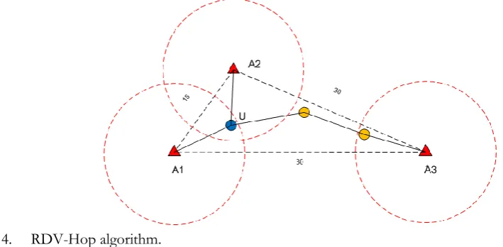
RSSI-based DV-Hop (RDV-Hop) localization algorithm is proposed as an enhancement to the traditional DV-Hop. It incorporates RSSI measurement and DV-Hop algorithm to implement localization. The aim is to reduce the location estimation error of unknown nodes, which are nearby some of the anchor nodes. In Fig. 4, A1, A2 and A3 are assumed to be all anchor nodes. Node U is an unknown node, which needs to obtain location.

Fig. 4. RDV-Hop algorithm.

In this example scenario, the actual distances between three anchor nodes are 15, 30, and 30. Every edge length is assumed to be 10. Like the DV-Hop algorithm, each anchor node will try to calculate the average distance per hop first. The average hop size of each anchor node in this case is the same value of 7.5. All the anchor nodes generate beacon packets to broadcast in the network, and any node receiving the packet can compute the distance from itself to the anchor using the measured RSSI.

In Fig. 4, node U is the one-Hop neighbor of nodes A1 and A2, that is to say, U can receive RSSI packets from A1 and A2 directly. After receiving the beacon packets with embedded RSSI values, U then computes the distance from A1 and A2 to itself, assuming the calculated values are 10 and 10. For the estimated distance from U to A3, the DV hop method is used. As a result, U can locate itself by using the triangulation method with the estimated distances to A1, A2, and A3 equal to 10, 10 and, 22.5 respectively.

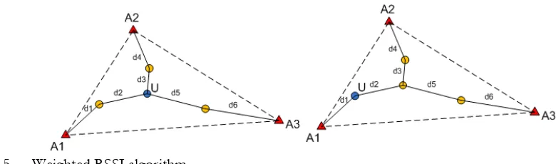
Weighted RSSI algorithm employs the summation of distances in any hop giving the distance information from anchor nodes. In Fig. 5, A1, A2 and A3 are assumed to be the anchor nodes with known locations. Node U is the unknown node, whose location needs to be obtained. All of the unknown nodes generate beacon packets and flood into the network. Then, any node receiving the packet from neighboring nodes computes the distance based on measured RSSI (RSSI-distance). As a result, each unknown node has the distances from itself to all its neighboring nodes. This also includes the distance to any anchor nodes, which are located within the radio radius of the unknown node. Then, an unknown node sums up the shortest-route distances from three anchor nodes. After receiving distances to the three nearest anchors, the trilateration method can be used to locate the unknown node’s position.

Fig. 5. Weighted RSSI algorithm.

These reference methods as well as the traditional DV-Hop have individual week points as discussed, and in this work we try to overcome. In the following sections, experimental and simulation results will be presented to show the performance comparison between these existing approaches and our proposed technique.

4.

RSSI Experiment and Simulation

From the theoretical understanding of distance estimation from RSSI measurement mentioned earlier, experiment has been setup in the laboratory environment to observe this behavior in comparison with simulation results. The testing environment is an uncontrolled environment with general usage of WiFi networks mimicking the possible actual usage environment of the WSN. In the experiment, the Digi International, Xbee Module Series 1 (1mW) [16], following the IEEE 802.15.4 standard, is used. The transmitted power used by the transceiver has been set to 1mW (0dBm) and frequency channel is set for channel 25 (central frequency = 2475MHz). One of the two modules (nodes) is set as an anchor node with fixed location in the lab. Initially, the other node (unknown node) was placed at 1-meter distance from the anchor node. Then, the unknown node was gradually moved to a 10-meter distance from the anchor node with a 1-meter step. The test scenario is shown in Fig. 6. The same scenario has been implemented by using MatLab simulation.

Fig. 6. RSSI measurement test scenario.

Fig. 7. Simulation results vs. testbed measurement results.

5.

Localization Simulation - Results and Discussion

A WSN-based simulation model has been developed to observe the performance of our proposed localization technique against existing approaches mentioned earlier. This simulation model has been initially verified with testbed results as discussed in the previous section. In order to see the effects of network density toward localization accuracy, two different network density levels are implemented.

5.1. Simulation of Low-Density WSN

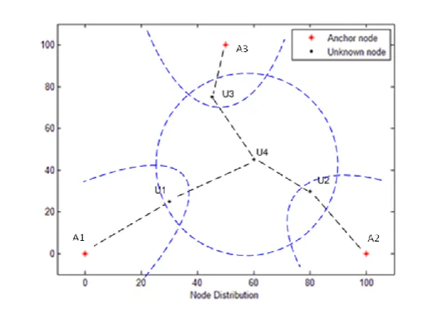
In this test, the simulation of WSN with low node density is performed. Nodes have been distributed in a large area in this simulation. Three anchor nodes and four unknown nodes were deployed in the area of 100 meters ×100 meters and the radio radius of 30 meters. The node distribution has been shown in Fig. 8 as well as the routes and the radio coverage. At least one unknown node should be located within anchor(s)’ radio radius.

Fig. 8. Node distributions for low-density WSN test case.

errors of the traditional Hop, RHop, weighted RSSI, and our proposed Selected RSSI-based DV-Hop algorithm (SRDV-DV-Hop) are 10.52, 8.42, 9.73, and 8.23 meters, respectively.

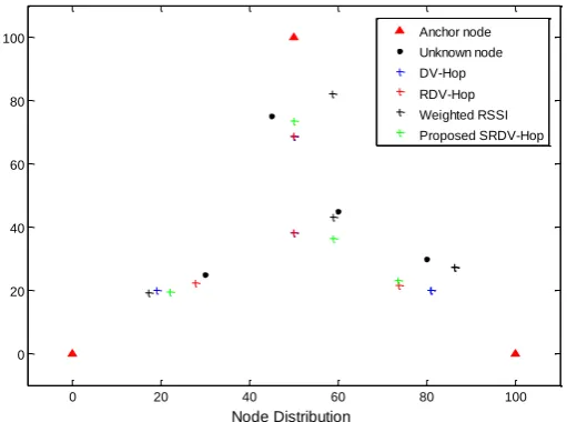
Fig. 9. The performance comparison for low-density WSN test case.

It can be seen from Fig. 9 that using the weighted RSSI algorithm, higher localization accuracy can only be achieved for unknown nodes located in the middle area of the test scenario, while the other nodes located nearer to the edge receive lower accuracy. This is because the large detour of the routes as explained in section three. From the results of average distance error for each technique, It is clear that the traditional DV-Hop and weighted RSSI algorithms have two largest errors of 10.52 and 9.73 meters, while our selected RSSI-based DV-Hop algorithm provides the lowest error of 8.23 meters. It is also noticeable that the error distances for each unknown node’s positions using our algorithm are almost equal.

5.2. Simulation of High-Density WSN

In this test, localization performance of the DV-Hop, RDV-Hop, and our proposed algorithm are evaluated via the developed simulation model for the high-density test scenario. It is assumed that the WSN is deployed in the square area with the fixed size. Sensor nodes are randomly distributed within the test area. One anchor node with fixed location in the middle, and four other anchor nodes are in four corners. The simulation parameters are summarized in Table 1. Two simulation scenarios are implemented. The major difference is the anchor node density, which is set to 5% in scenario one and 10% in scenario two. For each test, the RSSI error is varied from 1% to 30%. For each RSSI error, the simulations are performed 10 times.

Table 1. Simulation parameters for high-density WSN test case.

5.2.1. Scenario 1

Figures 10 and 11 display the simulation results obtained from the test scenario 1 with anchor node ratio of

0 20 40 60 80 100

0 20 40 60 80 100

Node Distribution

Anchor node Unknown node DV-Hop RDV-Hop Weighted RSSI Proposed SRDV-Hop

Parameter Scenario 1 Scenario 2

Percentage of Anchor Nodes 5% 10%

RSSI Error (%) 1-30% 1-30%

Radio Radius (m) 25 and 30 15 and 20

Node Number 100 50

In general, the distance error or localization error is usually defined as follows: assume that the real coordinate of the unknown node i is (x0,y0), and its estimated coordinate is (xi,yi), r is the communication range of unknown node, the localization error can be calculated from:



 



0 0

i i

i

x x y y

e

r

  

 (4)

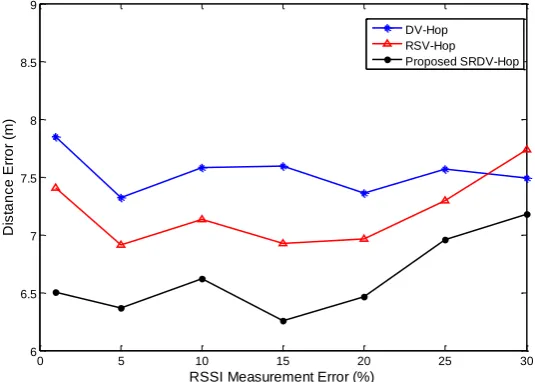
As seen in Fig. 10, the average distance error of DV-Hop algorithm is around 7.5 meters. This is because the RSSI measurement error does not affect the system accuracy. As a result, the distance error of DV-Hop algorithm remains almost stable as RSSI measurement error is changed. In contrast, the distance errors of RDV-Hop and the proposed SRDV-Hop algorithm increase moderately, when the RSSI measurement error increases.

Fig. 10. Simulation results for the performance comparison of test scenario 1 with radio radius of 25 meters.

For the RSSI measurement error of 1%, the SRDV-Hop algorithm provides a distance error of around 6.5 meters, while the traditional DV-Hop offers about 7.8 meters. The error difference between SRDV-Hop and DV-SRDV-Hop is almost 1.3 meters and between RDV-SRDV-Hop and DV-SRDV-Hop is almost 1 meter. At RSSI measurement error of 30%, the error of RDV-Hop algorithm exceeds the traditional DV-Hop, while the SRDV-Hop still offers the lowest value. Moreover, the proposed method offers the best accuracy in overall.

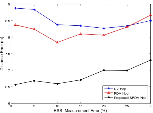
Figure 11 compares the distance error of DV-Hop, RDV-Hop and the proposed SRDV-Hop after increasing the radio radius in the simulator to 30 meters. It is clear that the difference between distance error obtained from SRDV-Hop and DV-Hop is larger than in the case of radio radius being 25 meters. When the RSSI measurement error is set to 1%, the difference in distance error between the SRDV-Hop and DV-Hop algorithm is about 2.3 meters. Note that this value for radio radius of 25 meters is 1.3 meters. Both DV-Hop and RDV-Hop algorithms provide higher distance error when the radio radius is 30 meters comparing with the error for the radio radius of 25 meters. This is because an unknown node can be located in a larger area under neighbor’s coverage while the number of hop counts may not change. Thus, this is the major problem affecting accuracy in the traditional DV-Hop algorithm. RDV-Hop offers slightly better accuracy due to the fact that it only improves the accuracy of small portion of nodes, which locates near anchor nodes. On the other hand, our proposed method offers rather similar range as radio radius is varied from 25 to 30 meters with a better overall accuracy.

0 5 10 15 20 25 30

6 6.5 7 7.5 8 8.5 9

D

is

ta

n

c

e

E

rr

o

r

(m

)

RSSI Measurement Error (%)

Fig. 11. Simulation results for the performance comparison of test scenario 1 with radio radius of 30 meters.

5.2.2. Scenario 2

Figures 12 and 13 show the simulation results obtained from the test scenario 2 with the anchor node ratio of 10% and radio radius of 15 and 20 meters, respectively. The figures show results in terms of average distance error in meter against RSSI measurement error.

Figure 12 compares the distance error against the RSSI measurement error of the three algorithms: DV-Hop, RDV-Hop and our SRDV-Hop algorithm as radio radius is set to 15 meters. It is obvious that the SRDV-Hop algorithm offers the lowest distance error, while the DV-Hop and RDV-Hop algorithms provide rather close results with high distance errors. The difference between the distance error of SRDV-Hop and DV-SRDV-Hop algorithms is about 1.2 meters compared with 0.2 meters, which is the difference between the RDV-Hop and DV-Hop algorithms.

Again, the DV-Hop algorithm maintains a rather similar result when the RSSI measurement error increases since the algorithm does not take into account RSSI measurement. On the other hand, RDV-Hop and SRDV-Hop algorithms are affected by this parameter. As a result, error increases noticeably as RSSI measurement error increases. The reason is because RSSI is conversed to distance in the first hop of anchor node in the RDV-Hop algorithm and in the radio radius of neighboring unknown nodes of SRDV-Hop algorithm. However, our proposed method provides a significant improvement with a much lower distance error in comparison with both DV-Hop and RDV-Hop algorithms for all values of RSSI measurement errors.

0 5 10 15 20 25 30

6 6.5 7 7.5 8 8.5 9

D

is

ta

n

c

e

E

rr

o

r

(m

)

RSSI Measurement Error (%)

Fig. 12. Simulation results for the performance comparison of test scenario 2 with radio radius of 15 meters.

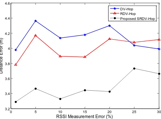
Figure 13 illustrates the simulation results for the distance error while the radio radius is set to 20 meters. It is clear that the distance error of DV-Hop algorithm is higher that than in Fig. 12, which is for the radio radius of 15 meters. This is because a larger radius allows an unknown node to be located in a larger area, however the number of hop count does not change. The difference between the distance error of SRDV-Hop and DV-Hop algorithm is larger than that in the case of radio radius being 15 meters.

In overall, the SRDV-Hop algorithm achieves the lowest distance error for all values of RSSI measurement error. DV-Hop algorithm offers the highest distance error at low RSSI measurement errors, however the distance errors obtained from RDV-Hop algorithm are the highest when the RSSI measurement error exceeds 20%.

Fig. 13. Simulation results for the performance comparison of test scenario 2 with radio radius of 20 meters.

Table 2 summarizes the simulation results and also illustrates the result of network density obtained from both test scenarios.

The network density is considered as one important aspect affecting the localization accuracy, and it is proposed by N. Bulusu [17] that localization algorithms are more effective when the network itself is dense. The network density, μ(R), can be expressed in terms of the number of nodes per nominal coverage area. Thus, if N nodes are scattered in a region of area A, and the nominal range of each node is R,

0 5 10 15 20 25 30

3.2 3.4 3.6 3.8 4 4.2 4.4 4.6 D is ta n c e E rr o r (m )

RSSI Measurement Error (%)

DV-Hop RDV-Hop Proposed SRDV-Hop

0 5 10 15 20 25 30

2.5 3 3.5 4 4.5 5 5.5 D is ta n c e E rr o r (m )

RSSI Measurement Error (%)

2 . .

N R

μ(R) A



 (5)

Note that the range R can be either the sensing range of a particular sensor or the radio transmission range (idealized with circular propagation). In each case, the associated network density will be different.

According to Eq. (4), the network density can be increased in many ways. In this simulation, it is increased by extending the radio radius (R) and the number of nodes (N), while maintaining the test space (A).In the test scenario one, it can be seen that when the radio radius, R, is increased from 25 to 30 meters, the network density (μ) also increases from 19.635 to 28.274. In contrast, the localization error decreases for all three localization algorithms. The result is also the same obtained from test scenario two.

Table 2. Network density and localization error with RSSI measurement error of 1%.

Scenario Percentage of anchor node

Radius (meter)

Network density

Localization Error

DV-Hop RDV-_Hop Proposed SRDV-Hop 1 5% 25 ₃₀ 19.635 _28.274 0.392 _0.293 0.298 _0.280 0.260 _0.217

2 10% 15 ₂₀ 14.137 _25.137 0.264 _0.212 0.252 _0.175 0.218 _0.137

It can be concluded that when the network density increases by increasing the radio radius, the localization error drops with the same percentage of anchor node. The SRDV-Hop algorithm offered the lowest localization error among the three algorithms for the same scenario and the same value of network density, while the DV-Hop algorithm provides the highest localization error.

6.

Conclusion

This paper presents a novel localization technique named as selected RSSI-based DV-Hop (SRDV-Hop), which enhances the basic DV-Hop algorithm by using RSSI measurement to calculate the first hop distances from the unknown nodes in combination with hop distance calculation of the traditional DV-Hop algorithm.

The performance evaluation was done via the developed simulation model. Initial test results were obtained via testbed experiment for simulation model evaluation, which show RSSI trend against distance in meter. Comparison results show that the trend of both tests is in the same way proving the credibility of the developed simulation model.

The simulations are separated into two major scenarios including WSN with low network density and WSN with high network density. The simulation results show that the proposed algorithm can improve localization accuracy in comparison with RDV-Hop and the traditional DV-Hop algorithms in both test scenarios (sparse and dense networks). As shown by the simulation results, it can be stated that the approach is effective and beneficial for many good application foregrounds. One additional conclusion gained from the experiment is that with fixed number of anchor nodes, when the network density increases (by increasing the radio radius), the localization error decreases. Moreover, the anchor density can also affect the localization error. It is shown in the simulation results that when the quantity of anchor nodes is increased as demonstrated by scenario two, the average localization error decreases.

References

[1] Y. Gu, A. Lo, and I. Niemegeers, “A survey of indoor positioning systems for wireless personal networks,” IEEE Communications Surveys & Tutorials, vol. 11, no. 1, pp. 13–32, 2009.

[2] M. Dru and S. Saada, “Location-based mobile services: The essentials,” Alcatel Telecommunications Review, pp. 71–76, 2001.

[5] N. A. Alsindi and K. Pahlavan, “Node localization,” Wireless Sensor Networks: A Networking Perspective, pp. 243-284, 2009.

[6] P. Kumar, L. Reddy, and S. Varma, “Distance measurement and error estimation scheme for RSSI based localization in wireless sensor networks,” in Proceeding of Fifth IEEE. Conference on Wireless Communication and Sensor Networks, Dec. 2009, pp. 1–4.

[7] R. Peng and M. L. Sichitiu, “Angle of arrival localization for wireless sensor networks,” in Annual IEEE Communications Society on Sensor and Ad Hoc Communications and Networks 2006, vol. 1, pp. 374–382. [8] P. J. Hernandez and D. Voltz “Maximum likelihood time of arrival estimation for real-time physical

location tracking of 802.11 a/g mobile stations in indoor environments,” in Proceeding of Position Localtion and Navigation Symposium (PLANS), California, USA, Apr. 2004. pp. 585–591.

[9] J. Ho and K. C. Kovavisaruch, “Alternate source and receiver location estimation using TDOA with receiver position uncertainties,” in Processing of IEEE International Conference on Acoustics, Speech, and Signal (ICASSP’05), Pennsylvania, USA, Mar. 2005, pp. 1065–1068.

[10] B. Nath and D Nicolescu, “Ad-hoc positioning systems (APS),” in Proceedings of Telecommunication Systems, Nov. 2001, vol. 5, pp. 2926–2931.

[11] N. Bulusu, J. Heidemann, and D. Estrin. “GPS-less low cost outdoor localization for very small devices,” IEEE Personal Communications Magazine, vol. 7, no. 5, pp. 28–34, Oct. 2000.

[12] T. He, C. Huang, B. M. Blum, J. A. Stankovic, and T Abdelzaher, “Range-free localization schemes for large scale sensor networks,” in Proceedings of the 9th Annual International Conference on Mobile Computing And Networking, ACM, 2003 (MobiCom’03), San Diego, California, USA, Sept. 2003, p. 81–95. [13] T. S. Rappaport, Wireless Communications: Principles and Practice, 2nd ed. Prentice Hall PTR, 2001.

[14] N. Bulusu, J. Heidemann, and D. Estrin, “Density adaptive algorithms for beacon placement in wireless sensor networks,” in Proceeding of IEEE ICDCS’01, Phoenix, Arizon, April 2001.

[15] P. X. Liu, X. M. Zhang, S. Tian, Z. W. Zhoa, and P. Sun, “A RSSI-based DV-Hop algorithm for wireless sensor networks,” in Proceeding Of IEEE WICOM 2007, September, 2007, pp. 2555–2558. [16] Digi International - Overview and Specification for XBee® 802.15.4. [Online]. Available:

http://www.digi.com