Generalized Hierarchical Kernel Learning
Pratik Jawanpuria [email protected]
Jagarlapudi Saketha Nath [email protected]
Ganesh Ramakrishnan [email protected]
Department of Computer Science and Engineering Indian Institute of Technology Bombay
Mumbai 400076, INDIA
Editor:Francis Bach
Abstract
This paper generalizes the framework of Hierarchical Kernel Learning (HKL) and illustrates its utility in the domain of rule learning. HKL involves Multiple Kernel Learning over a set of given base kernels assumed to be embedded on a directed acyclic graph. This paper proposes a two-fold generalization of HKL: the first is employing a generic `1/`ρ block-norm regularizer (ρ∈(1,2]) that alleviates a key limitation of the HKL formulation. The second is a generalization to the case of multi-class, multi-label and more generally, multi-task applications. The main technical contribution of this work is the derivation of a highly specialized partial dual of the proposed generalized HKL formulation and an efficient mirror descent based active set algorithm for solving it. Importantly, the generic regularizer enables the proposed formulation to be employed in the Rule Ensemble Learning (REL) where the goal is to construct an ensemble of conjunctive propositional rules. Experiments on benchmark REL data sets illustrate the efficacy of the proposed generalizations.
Keywords: multiple kernel learning, mixed-norm regularization, multi-task learning, rule ensemble learning, active set method
1. Introduction
A Multiple Kernel Learning (MKL) (Lanckriet et al., 2004; Bach et al., 2004) framework for construction of sparse linear combinations of base kernels embedded on a directed acyclic graph (DAG) was recently proposed by Bach (2008). Since the DAG induces hierarchical relations between the base kernels, this framework is more commonly known as Hierarchical Kernel Learning (HKL). It has been established that HKL provides a powerful algorithm for task specific non-linear feature selection. HKL employs a carefully designed`1/`2
block-norm regularizer: `1-norm across some predefined components associated with the DAG and`2-norm within each such component. However, the sparsity pattern of kernel (feature) selection induced by this regularizer is somewhat restricted: a kernel is selected only if the kernels associated with all its ancestors in the DAG are selected. In addition, it can be proved that the weight of the kernel associated with a (selected) node will always be greater than the weight of the kernels associated with its descendants. Such a restricted selection pattern and weight bias may limit the applicability of HKL in real world problems.
This paper proposes a two-fold generalization of HKL. The first is employing a`1/`ρ, ρ∈
among the kernels, henceforth termed as gHKL. Note that for the special case of ρ = 2, gHKL renders the HKL regularizer. Further, gHKL is generalized to the paradigm of Multi-task Learning (MTL), where multiple related Multi-tasks need to be learnt jointly. We consider the MTL setup where the given learning tasks share a common sparse feature space (Lounici et al., 2009; Jawanpuria and Nath, 2011; Obozinski et al., 2011). Our goal is to construct a shared sparse feature representation that is suitable for all the given related tasks. We pose the problem of learning this shared feature space as that of learning a shared kernel, common across all the tasks. The proposed generalization is henceforth referred to as gHKLMT. In
addition to learning a common feature representation, gHKLMT is generic enough to model
additional correlations existing among the given tasks.
Though employing a `1/`ρ, ρ∈(1,2), regularizer is an incremental modification to the
HKL formulation, devising an algorithm for solving it is not straightforward. The projected gradient descent employed in the active set algorithm for solving HKL (Bach, 2008) can no longer be employed for solving gHKL as projections onto `ρ-norm balls are known to be
significantly more challenging than those onto`1-norm balls (Liu and Ye, 2010). Hence naive extensions of the existing HKL algorithm will not scale well. Further, the computational challenge is compounded with the generalization for learning multiple tasks jointly. The key technical contribution of this work is the derivation of a highly specialized partial dual of the gHKL/gHKLMT formulations and an efficient mirror descent (Ben-Tal and
Nemirovski, 2001; Beck and Teboulle, 2003) based active set algorithm for solving it. The dual presented here is an elegant convex optimization problem with a Lipschitz continuous objective and constrained over a simplex. Moreover, the gradient of the objective can be obtained by solving a known and well-studied variant of the MKL formulation. This motivates employing the mirror descent algorithm that is known to solve such problems efficiently. Further efficiency is brought in by employing an active set method similar in spirit to that in Bach (2008).
A significant portion of this paper focuses on the application of Rule Ensemble Learn-ing (REL) (Dembczy´nski et al., 2010, 2008), where HKL has not been previously explored. Given a set of basic propositional features describing the data, the goal in REL is to con-struct a compact ensemble of conjunctions with the given propositional features that gen-eralizes well for the problem at hand. Such ensembles are expected to achieve a good trade-off between interpretability and generalization ability. REL approaches (Cohen and Singer, 1999; Friedman and Popescu, 2008; Dembczy´nski et al., 2010) have additionally addressed the problem of learning a compact set of rules that generalize well in order to maintain their readability. One way to construct a compact ensemble is to consider a linear model involving all possible conjunctions of the basic propositional features and then per-forming a `1-norm regularized empirical risk minimization (Friedman and Popescu, 2008;
with such a setup, the size of the gHKL optimization problem is exponential in the number of basic propositional features. However, a key result in the paper shows that the proposed gHKL algorithm is guaranteed to solve this exponentially large problem with a complexity polynomial in the final active set1 size. Simulations on benchmark binary (and multiclass) classification data sets show that gHKL (and gHKLMT) indeed constructs a compact
en-semble that on several occasions outperforms state-of-the-art REL algorithms in terms of generalization ability. These results also illustrate the benefits of the proposed generaliza-tions over HKL: i) the ensembles constructed with gHKL (with lowρ values) involve fewer number of rules than with HKL; though the accuracies are comparable ii) gHKLMT can
learn rule ensemble on multiclass problems; whereas HKL is limited to two-class problems. The rest of the paper2 is organized as follows. Section 2 introduces the classical Multi-ple Kernel Learning setup, briefly reviews the HKL framework and summarizes the existing works in Multi-task Learning. In Section 3, we present the proposed gHKL and gHKLMT
formulations. The key technical derivation of the specialized dual is also presented in this section. The proposed mirror descent based active set algorithm for solving gHKL/gHKLMT
formulations is discussed in Section 4. In Section 5, we propose to solve the REL problem by employing the gHKL formulation and discuss its details. In Section 6, we report em-pirical evaluations of gHKL and gHKLMT formulations for REL on benchmark binary and
multiclass data sets respectively. Section 7 concludes the paper.
2. Related Works
This section provides a brief introduction to the Multiple Kernel Learning (MKL) frame-work, the HKL setup and formulation (Bach, 2008, 2009) as well as the existing works in Multi-task Learning.
2.1 Multiple Kernel Learning Framework
We begin by discussing the regularized risk minimization framework (Vapnik, 1998), which has been employed in the proposed formulations.
Consider a learning problem like classification or regression and let its training data be denoted byD={(xi, yi), i= 1, . . . , m |xi ∈ X, yi∈R∀i}, where (xi, yi) represents the ith
input-output pair. The aim is to learn an affine prediction function F(x) that generalize well on unseen data. Given a positive definite kernelkthat induces a feature mapφk(·), the
prediction function can be written as: F(x) =hf, φk(x)iHk−b. HereHkis the Reproducing Kernel Hilbert Space (RKHS) (Sch¨olkopf and Smola, 2002) associated with the kernel k, endowed with an inner product h·,·iHk, and f ∈ Hk, b ∈ R are the model parameters to be learnt. A popular framework to learn these model parameters is the regularized risk minimization (Vapnik, 1998), which considers the following problem:
min
f∈Hk,b∈R
1 2Ω(f)
2+C
m
X
i=1
`(yi, F(xi)), (1)
1. Roughly, this is the number of selected conjunctions and is potentially far less than the total number of conjunctions.
where Ω(·) is a norm based regularizer,`:R×R→Ris a suitable convex loss function andC is a regularization parameter. As an example, the support vector machine (SVM) (Vapnik, 1998) employs Ω(f) =kfkHk. From therepresenter theorem (Sch¨olkopf and Smola, 2002), we know that the optimalf has the following form f(·) =Pm
i αik(·,xi) where α= (αi)mi=1
is a vector of coefficients to be learnt.
It can be observed from above that the kernel definition plays a crucial role in defining the quality of the solution obtained by solving (1). Hence learning a kernel suitable to the problem at hand has been an active area of research over the past few years. One way to learn kernels is via the Multiple Kernel Learning (MKL) framework (Lanckriet et al., 2004; Bach et al., 2004). Lanckriet et al. (2004) proposed to learn the kernel k as a conic combination of the given base kernelsk1, . . . , kl: k=Pli=1ηiki, ηi≥0∀i. Hereη= (ηi)li=1
is a coefficient vector to be (additionally) learnt in the optimization problem (1). In this setting, the feature map with respect to the kernel k is given by φk = (
√ ηiφki)
l
i=1 (see
Rakotomamonjy et al., 2008, for details). It is a weighted concatenation of feature maps induced by the individual base kernels. Hence, sparse kernel weights will result in a low dimensionalφk. Some of the additional constraints onηexplored in the existing MKL works
are`1-norm constraint (Bach et al., 2004; Rakotomamonjy et al., 2008),`p-norm constraint
(p >1) (Kloft et al., 2011; Vishwanathan et al., 2010; Aflalo et al., 2011), etc.
2.2 Hierarchical Kernel Learning
Hierarchical Kernel Learning (HKL) (Bach, 2008) is a generalization of MKL and assumes a hierarchy over the given base kernels. The base kernels are embedded on a DAG and a carefully designed `1/`2 block-norm regularization over the associated RKHS is proposed
to induce a specific sparsity pattern over the selected base kernels. We begin by discussing its kernel setup.
Let G(V,E) be the given DAG with V denoting the set of vertices and E denoting the set of edges. The DAG structure entails relationships like parent, child, ancestor and descendant (Cormen et al., 2009). LetD(v) andA(v) represent the set of descendants and ancestors of the node v in the G. It is assumed that both D(v) and A(v) include the node
v. For any subset of nodesW ⊂ V, thehull and sourcesof W are defined as:
hull(W) = [
w∈W
A(w), sources(W) ={w∈ W |A(w)∩ W={w}}.
The size and complement ofW are denoted by|W|andWcrespectively. Letk
v :X ×X →R be the positive definite kernel associated with the vertex v ∈ V. In addition, let Hkv be its associated RKHS and φkv be its induced feature map. Given this, HKL employs the following prediction function:
F(x) =X
v∈V
hfv, φkv(x)iHkv −b,
which is an affine model parameterized by f = (fv)v∈V, the tuple with entries as fv ∈ Hkv and b ∈ R. Some more notations follow: for any subset of nodes W ⊂ V, fW = (fv)v∈W and φW = (φv)v∈W. In general, the entries in a vector are referred to using an appropriate subscript, i.e., entries inu∈Rd are denoted by u1, . . . , ud. The kernels are denoted by the
HKL formulates the problem of learning the optimal prediction function F as the fol-lowing regularized risk minimization problem:
min
fv∈Hkv∀v∈V,b∈R
1 2
X
v∈V
dvkfD(v)k2
!2 +C
m
X
i=1
`(yi, F(xi)), (2)
where kfD(v)k2 =
P
w∈D(v)kfwk2
12
∀v ∈ V,`(·,·) is a suitable convex loss function and
(dv)v∈V are given non-negative parameters.
As is clear from (2), HKL employs a `1/`2 block-norm regularizer, which is known to promote group sparsity (Yuan and Lin, 2006). Its implications are discussed in the following. For most of v ∈ V, kfD(v)k2 = 0 at optimality due to the sparsity inducing
nature of the `1-norm. Moreover (kfD(v)k2 = 0) ⇒ (fw = 0 ∀w ∈ D(v)). Thus it is
expected that most fv will be zero at optimality. This implies that the prediction function
involves very few kernels. Under mild conditions on the kernels (being strictly positive), it can be shown that this hierarchical penalization induces the following sparsity pattern: (fw 6= 0)⇒(fv 6= 0∀v∈A(w)). In other words, if the prediction function employs a kernel
kw then it certainly employsallthe kernels associated with the ancestor nodes of w.
Bach (2008) proposes to solve the following equivalent variational formulation:
min
γ∈∆1
min
fv∈Hkv∀v∈V,b∈R
1 2
X
w∈V
δw(γ)−1kfwk2+C m
X
i=1
`(yi, F(xi)), (3)
where ∆1 =
z∈R|V| |z≥0,P
v∈Vzv ≤1 and δw(γ)−1 = Pv∈A(w)
d2
v
γv. From the repre-senter theorem (Sch¨olkopf and Smola, 2002), it follows that the effective kernel employed in the HKL is: k = P
w∈Vδw(γ)kw. Since the optimization problem (3) has a `1-norm
constraint over γ variables, most γv at optimality are expected to be zero. Moreover the
kernel weight δw(γ) is zero whenever γv = 0 for any v ∈ A(w). Thus, the HKL performs
a sparse selection of the base kernels and can be understood as a generalization of the classical MKL framework. However, the sparsity pattern for the kernels has the following restriction: if a kernel is not selected then none of the kernels associated with its descen-dants are selected, as (γv = 0)⇒ (δw(γ) = 0 ∀w∈D(v)). For the case of strictly positive
kernels, it follows that a kernel is selected only if all the kernels associated with its ances-tors are selected. In addition, the following relationship holds among the kernels weights:
δv(γ) ≥δw(γ) ∀w ∈ D(v) (strict inequality holds if δw(γ) > 0). Hence, the weight of the
kernel associated with a (selected) node is always be greater than the weight of the kernels associated with its descendants.
Since the size ofγis same as that ofVand since the optimalγ is known to be sparse, Bach (2008) proposes an active set based algorithm (Lee et al., 2007) for solving (3). At each iteration of the active set algorithm, (3) is solved with respect to only those variables in the active set via the projected gradient descent technique (Rakotomamonjy et al., 2008).
the promising sub-products of the input features over all possible sub-products. Please refer to Bach (2008) for more such pragmatic examples of kernels and corresponding DAGs. The most interesting result in Bach (2008) is that in all these examples where the size of the DAG is exponentially large, the computational complexity of the active set algorithm is polynomial in the training set dimensions and the active set size. Importantly, the complexity is independent of|V|!
Though encouraging, the above discussed weight bias (in favor of the kernels towards the top of the DAG) and restricted kernel selection pattern may limit the applicability of HKL in real world problems. For instance, in case of the sub-product kernel example mentioned above, the following is true: a sub-product is selected only if all the products including it are selected. This clearly may lead to selection of many redundant sub-products (features). In Section 3, we present the proposed generalization that provides a more flexible kernel selection pattern by employing a `1/`ρ, ρ ∈(1,2), regularizer. A key result of this
paper (refer Corollary 6) is that for all the cases discussed in Bach (2008), the proposed mirror descent based active set algorithm for solving the generalization has a computational complexity that is still polynomial in the training set dimensions and the active set size. In other words, the proposed generalization does not adversely affect the computational feasibility of the problem and hence is an interesting result in itself.
2.3 Multi-task Learning
Multi-task Learning (Caruana, 1997; Baxter, 2000) focuses on learning several prediction tasks simultaneously. This is in contrast with the usual approach of learning each task separately and independently. The key underlying idea behind MTL is that an appropriate sharing of information while learningrelated tasks will help in obtaining better prediction models. Various definitions of task-relatedness have been explored over the past few years like proximity of task parameters (Baxter, 2000; Evgeniou and Pontil, 2004; Xue et al., 2007; Jacob et al., 2008; Jawanpuria and Nath, 2012) or sharing common feature space (Ando and Zhang, 2005; Ben-David and Schuller, 2008; Argyriou et al., 2008; Lounici et al., 2009; Obozinski et al., 2011). Many learning settings like multiclass classification, multi-label classification or learning vector-valued function may be viewed as a special case of multi-task learning.
In this work, we consider the common setting in which the task parameters share a simul-taneously sparse structure: only a small number of input features are relevant for each of the tasks and the set of such relevant features is common across all the tasks (Turlach et al., 2005; Lounici et al., 2009). Existing works in this setting typically employ a group lasso penalty on the tasks parameters: `1/`2 block-norm (Lounici et al., 2009; Obozinski et al., 2011) or
the`1/`∞ block-norm (Turlach et al., 2005; Negahban and Wainwright, 2009). Thus, they
propose a multi-task regularizer of the form: Ω(f1, . . . , fT) =
Pd
i=1
PT
t=1|fti|q
1 q
where the input feature space is assumed to be d dimensional, ft is the task parameter of the
tth task and ft = (fti)i=1,...,d and q = {2,∞}. Note that in addition to (sparse) shared
feature selection, the `1/`∞ block-norm penalty also promote proximity among the task parameters.
constructed as a sparse combination of the given base kernels. A hierarchical relationship exists over the given kernels (feature spaces). We employ a graph based `1/`ρ block-norm
regularization over the task parameters that enable non-linear feature selection for multiple tasks simultaneously. The details of the proposed MTL formulation are discussed in the following section.
3. Generalized Hierarchical Kernel Learning
In this section, we present the proposed generalizations over HKL. As discussed earlier, the first generalization aims at mitigating the weight bias problem as well as the restrictions imposed on the kernel selection pattern of HKL, and is termed as gHKL. The gHKL formu-lation is then further generalized to the paradigm of MTL, the proposed formuformu-lation being termed as gHKLMT. We begin by introducing the gHKL formulation.
3.1 gHKL Primal Formulation
Recall that HKL employs a`1/`2 block norm regularizer. As we shall understand in more detail later, a key reason for the kernel weight bias problem and the restricted sparsity pattern in HKL is the `2-norm regularization. One way to mitigate these restrictions is by
employing the following generic regularizer:
ΩS(f) =
X
v∈V
dvkfD(v)kρ, (4)
where f = (fv)v∈V, kfD(v)kρ =
P
w∈D(v)kfwkρ
1 ρ
and ρ ∈(1,2]. The implications of the
`1/`ρblock-norm regularization are discussed in the following. Since the `1-norm promotes
sparsity, it follows that kfD(v)kρ = 0 (that is fw = 0 ∀w ∈ D(v)) for most v ∈ V. This
phenomenon is similar as in HKL. But now, even in cases where kfD(v)kρ is not forced to
zero by the `1-norm, many components of fD(v) tend to zero3 (that is fw → 0 for many
w∈D(v)) as the value ofρtends to unity. Also note thatρ= 2 renders the HKL regularizer. To summarize, the proposed gHKL formulation is
min
fv∈Hkv∀v∈V,b∈R
1
2(ΩS(f))
2+C
m
X
i=1
`(yi, F(xi)). (5)
We next present the gHKLMTformulation, which further generalizes gHKL to MTL paradigm.
3.2 gHKLMT Primal Formulation
We begin by introducing some notations for the multi-task learning setup. Let T be the number of tasks and let the training data for thetthtask be denoted byDt={(xti, yti), i=
1, . . . , m | xti ∈ X, yti ∈R ∀i}, where (xti, yti) represents the ith input-output pair of the
3. Note that as`ρ-norm (ρ >1) is differentiable, it rarely induce sparsity (Szafranski et al., 2010). However,
as ρ→1, they promote only a few leading terms due to the high curvatures of such norms (Szafranski et al., 2007). In order to obtain a sparse solution in such cases, thresholding is commonly employed by existing`p-MKL (ρ >1) algorithms (Vishwanathan et al., 2010; Orabona et al., 2012; Jain et al., 2012;
tth task. For the sake of notational simplicity, it is assumed that the number of training examples is same for all the tasks. The prediction function for the tth task is given by:
Ft(x) =
P
v∈Vhftv, φkv(x)iHkv −bt, where ft = (ftv)v∈V and bt are the task parameters to be learnt. We propose the following regularized risk minimization problem for estimating these task parameters and term it as gHKLMT:
min
ft,bt∀t 1 2 X v∈V dv X
w∈D(v)
(Qw(f1, . . . , fT))ρ
1
ρ
| {z }
ΩT(f1,...,fT)
2 +C T X t=1 m X i=1
`(yti, Ft(xti)), (6)
where ρ ∈ (1,2] and Qw(f1, . . . , fT) is a norm-based multi-task regularizer on the task
parameters ftw ∀t . In the following, we discuss the effect of the above regularization.
Firstly, there is a `1-norm regularization over the group of nodes (feature spaces) and a `ρ-norm regularization within each group. This`1/`ρ block-norm regularization is same as
that of gHKL and will have the same effect on the sparsity pattern of the selected feature spaces (kernels). Hence, only a few nodes (feature spaces) will be selected by the gHKLMT
regularizer ΩT(f1, . . . , fT). Secondly, nature of the task relatedness within each (selected)
feature space is governed by the Qw(f1, . . . , fT) regularizer.
For instance, consider the following definition of Qw(f1, . . . , fT) (Lounici et al., 2009;
Jawanpuria and Nath, 2011):
Qw(f1, . . . , fT) = T
X
t=1 kftwk2
!12
. (7)
The above regularizer couples the task parameters within each feature space via`2-norm. It
encourages the task parameters within a feature space to be either zero or non-zero across all the tasks. Therefore, ΩT(f1, . . . , fT) based on (7) has the following effect: i) all the tasks
will simultaneously select or reject a given feature space, and ii) overall only a few feature spaces will be selected in the gHKL style sparsity pattern.
Several multi-task regularizations (Evgeniou and Pontil, 2004; Evgeniou et al., 2005; Jacob et al., 2008) have been proposed to encourage proximity among the task parameters within a given feature space. This correlation among the tasks may be enforced while learning a shared sparse feature space by employing the following Qw(f1, . . . , fT):
Qw(f1, . . . , fT) =
µ 1
T +µ
T X t=1 ftw 2 + T X t=1
ftw−
1
T+µ
T X t=1 ftw 2 1 2 , (8)
whereµ >0 is a given parameter. The aboveQw(f1, . . . , fT) consists of two terms: the first
regularizes the mean while the second regularizes the variance of the task parameters in the feature space induced by kernel kw. The parameterµ controls the degree of proximity
among the task parameters, with lower µ encouraging higher proximity. Note that when
following effect: i) all the tasks will simultaneously select or reject a given feature space, ii) overall only a few feature spaces will be selected in the gHKL style sparsity pattern, and iii) within each selected feature space, the task parameters ftw ∀tare in proximity.
Thus, gHKLMT framework provides a mechanism to learn a shared feature space across
the tasks. In addition, it can also preserve proximity among the tasks parameters in the learnt feature space. As we shall discuss in the next section, more generic correlations among task parameters may be also modeled within the gHKLMT framework.
It is clear that the gHKL optimization problem (5) may be viewed as a special case of the gHKLMT optimization problem (7), with the number of tasks set to unity. Hence
the rest of the discussion regarding dual derivation and optimization focuses primarily on gHKLMT formulation.
3.3 gHKLMT Dual Formulation
As mentioned earlier, due to the presence of the `ρ-norm term in gHKLMT formulation,
naive extensions of the projected gradient based active set method in Bach (2008) will be rendered computationally infeasible on real world data sets. Hence, we first re-write gHKLMT formulation in an elegant form, which can then be solved efficiently. To this end,
we note the following variational characterization of ΩT(f1, . . . , fT).
Lemma 1 Given ΩT(f1, . . . , fT) andQw(f1, . . . , fT) as defined in (6) and (8) respectively, we have:
ΩT(f1, . . . , fT)2 = min
γ∈∆ λv∈∆minvρˆ ∀v∈V X
w∈V
δw(γ, λ)−1Qw(f1, . . . , fT)2, (9)
where ρˆ = 2−ρρ, δw(γ, λ)−1 = Pv∈A(w)
d2
v
γvλvw, ∆1 =
z∈R|V| |z≥0,P
v∈Vzv ≤1 and
∆vr = n
z∈R|D(v)| |z≥0,Pw∈D(v)zrw ≤1
o
.
Note that ρ ∈ (1,2) ⇒ ρˆ ∈ (1,∞). The proof of the above lemma is provided in Ap-pendix A.2.
In order to keep the notations simple, in the remainder of this section, it is assumed that the learning tasks at hand are binary classification, i.e., yti ∈ {−1,1} ∀t, i, and the
loss function is the hinge loss. However, one can easily extend these ideas to other loss functions and learning problems. Refer Appendix A.8 for gHKLMT dual formulation with
general convex loss functions.
Lemma 2 Consider problem (6) with the regularizer term replaced with its variational char-acterization (9) and the loss function as the hinge loss `(y, Ft(x)) = max (0,1−yFt(x)). Then the following is a partial dual of it with respect to the variablesft, bt ∀t= 1, . . . , T:
min
γ∈∆1
min
λv∈∆vρˆ ∀v∈V
max
αt∈S(yt,C)∀t
G(γ, λ, α), (10)
where
G(γ, λ, α) =1>α− 1
2α
>Y X
w∈V
δw(γ, λ)Hw
!
α= [α>1, . . . , α>T]>,S(yt, C) ={β ∈Rm |0≤β ≤C, Pmi=1ytiβi = 0}, yt= [yt1, . . . , ytm]>,
Y is the diagonal matrix corresponding to the vector [y>1, . . . ,y>T]>, 1 is a mT ×1 vector with entries as unity, δw(γ, λ)−1 =Pv∈A(w)
d2
v
γvλvw, ∆1 =
z∈R|V| |z≥0,P
v∈Vzv ≤1 ,
∆v r =
n
z∈R|D(v)| |z≥0,P
w∈D(v)zrw ≤1
o
,ρˆ= 2−ρρ, andHw ∈RmT×mT is the multi-task
kernel matrix corresponding to the multi-task kernel hw ∀w∈ V. The kernel functionhw is defined as follows:
hw(xt1i,xt2j) =kw(xt1i,xt2j)B(t1, t2), (11)
where B is a T ×T matrix. B = I (identity matrix) when the multi-task regularizer (7) is employed in (6). Alternatively, B = I +11>/µ (here 1 is a T ×1 vector with entries as unity) in the case when the regularizer (8) is employed. The prediction function for the task t1 is given by
Ft1(xt1j) =
T
X
t2=1
m
X
i=1
¯
αt2iyt2i
X
w∈V
δw(¯γ,λ¯)kw(xt1i,xt2j)B(t1, t2)
!
,
where (¯γ,λ,¯ α¯) is an optimal solution of (10).
Proof The proof follows from the representer theorem (Sch¨olkopf and Smola, 2002). Also refer to Appendix A.3.
This lemma shows that gHKLMT essentially constructs the same prediction function as an
SVM with the effective multi-task kernel as: h =P
w∈Vδw(γ, λ)hw. Similarly, in the case
of the gHKL, the effective kernel is k = P
w∈Vδw(γ, λ)kw (since the terms T and B are
unity). Here, as well as in the rest of the paper, we employ the symbols ‘h’ and ‘H’ for the multi-task kernel and the corresponding Gram matrix respectively.
The multi-task kernel (11) consists of two terms: the first term corresponds to the similarity between two instances xt1i and xt2j in the feature space induced by the kernel
kw. The second term corresponds to the correlation between the taskst1 andt2. In the case
of the regularizer (7), the matrix B simplifies to: B(t1, t2) = 1 if t1 =t2 and B(t1, t2) = 0 if t1 6= t2, thereby making the kernel matrices Hw(w ∈ V) block diagonal. Hence, the
gHKLMT regularizer based on (7) promotes simultaneous sparsity in kernel selection among
the tasks, without enforcing any additional correlations among the tasks.
In general, any T ×T positive semi-definite matrix may be employed as B to model generic correlations among tasks. The multi-task kernel given by (11) will still remain a valid kernel (Sheldon, 2008; ´Alvarez et al., 2012). The matrixB is sometimes referred to as the output kernel in the setting of learning vector-valued functions. It is usually constructed from the prior domain knowledge.
We now discuss the nature of the optimal solution of (10). Most of the kernel weights
δw(γ, λ) are zero at optimality of (10): δw(γ, λ) = 0 whenever γv = 0 or λvw = 0 for
any v ∈ A(w). The vector γ is sparse due to `1-norm constraint in (10). In addition, ρ → 1⇒ ρˆ→1. Hence the vectors λv ∀v∈ V get close to becoming sparse as ρ →1 due
flexible4 sparsity pattern in kernel selection. This is explained in detail towards the end of this section.
Note that ρ = 2 ⇒ λvw = 1 ∀v ∈ A(w), w ∈ W at optimality in (10). Hence for
ρ= 2, the minimization problem in (10) can be efficiently solved using a projected gradient method (Rakotomamonjy et al., 2008; Bach, 2009). However, as established in Liu and Ye (2010), projection onto the kind of feasibility set in the minimization problem in (10) is computationally challenging for ρ ∈ (1,2). Hence, we wish to re-write this problem in a relatively simpler form that can be solved efficiently. To this end, we present the following important theorem.
Theorem 3 The following is a dual of (6) considered with the hinge loss function, and the objectives of (6) (with the hinge loss), (10) and (12) are equal at optimality:
min
η∈∆1
g(η), (12)
where g(η) is the optimal objective value of the following convex problem:
max
αt∈S(yt,C)∀t
1>α−1
2 X
w∈V
ζw(η)
α>YHwYα
ρ¯ !ρ1¯
, (13)
where ζw(η) =
P
v∈A(w)d
ρ vηv1−ρ
1−1ρ
, α = [α>1, . . . , α>T]>, S(yt, C) = {β ∈ Rm | 0 ≤
β ≤ C, Pm
i=1ytiβi = 0}, yt = [yt1, . . . , ytm]
>, Y is the diagonal matrix corresponding to
the vector [y>1, . . . ,y>T]>, 1 is a mT ×1 vector with entries as unity, ρ¯ = ρˆ−ρˆ1, ρˆ = 2−ρρ,
∆1 =
z∈R|V| |z≥0,P
v∈Vzv ≤1 , and Hw ∈RmT×mT is the multi-task kernel matrix
corresponding to the multi-task kernel (11).
The key idea in the proof of the above theorem is to eliminate theλvariables and the details are presented in Appendix A.5. The expression for the prediction function F, in terms of the variablesη and α, is provided in Appendix A.9.
This theorem provides some key insights: firstly, we have that (12) is essentially a `1 -norm regularized problem and hence it is expected that mostη will be zero at optimality. Since (ηv = 0) ⇒ (ζw(η) = 0 ∀w ∈ D(v)), it follows that most nodes in V will not
contribute in the optimization problems (12) and (13). Secondly, in a single task learning setting (T = 1), the problem in (13) is equivalent to the`ρˆ-norm MKL dual problem (Kloft
et al., 2011) with the base kernels as (ζv(η))
1 ¯
ρk
v ∀v ∈ V 3 ζv(η) 6= 0. The optimization
problem (13) essentially learns an effective kernel of the form h = P
v∈Vθv(ζv(η))
1 ¯
ρhv, where theθ are intermediate optimization variables constrained to be non-negative and lie within a`ˆρ-norm ball. The expression forθin terms of the variables ηand αis provided in
Appendix A.9.
The variable θ influence the nature of the effective kernel h in two important ways: i) it follows from the expression ofθ that
θv(ζv(η))
1 ¯
ρ ∝ζ
v(η)
α>YHvYα
( ˆρ−11)
.
4. The HKL dual formulation (Bach, 2009) is a special case of (10) withρ= 2,T = 1 and B= 1. When
ρ = 2, ˆρ =∞. This impliesλvw = 1∀ v∈ A(w), w ∈ V at optimality, resulting in the weight bias
Algorithm 1 Active Set Algorithm - Outline
Input: Training dataD, the kernels (kv) embedded on the DAG (V), the T ×T matrix
B that models task correlations and tolerance . Initialize the active set W withsources(V). Compute η, α by solving (14)
while Optimal solution for (12) is NOT obtaineddo Add somenodes toW
Recomputeη, α by solving (14) end while
Output: W, η, α
The above relation implies that the weight of the kernel hv in the DAG V is not only
dependent on the position5 of the node v, but also on the suitability of the kernel hv to
the problem at hand. This helps in mitigating the kernel weight bias in favour of the nodes towards the top of the DAG from gHKLMT, but which is present in HKL, and ii) asρ→1
(and hence as ˆρ→ 1), the optimal θ get close to becoming sparse (Szafranski et al., 2007; Orabona et al., 2012). This superimposed with the sparsity of η promotes a more flexible sparsity pattern in kernel selection that HKL, especially whenρ→1.
Next, we propose to solve the problem (12) by exploiting the sparsity pattern of the
η variables and the corresponding ζ(η) terms at optimality. We discuss it in detail in the following section.
4. Optimization Algorithm
Note that problem (12) remains the same whether solved with the original set of variables (η) or when solved with only those ηv 6= 0 at optimality (refer Appendix A.4 for details).
However the computational effort required in the latter case can be significantly lower since it involves low number of variables and kernels. This motivates us to explore an active set algorithm, which is similar in spirit to that in Bach (2008).
An outline of the proposed active set algorithm is presented in Algorithm 1. The algo-rithm starts with an initial guess for the setW such thatηw6= 0 (∀w∈ W) at the optimality
of (12). This setW is called the active set. Since the weight associated with the kernelhw
will be zero whenever ηv = 0 for anyv∈A(w), the active setW must containsources(V),
else the problem has a trivial solution. Hence, the active set is initialized withsources(V). At each iteration of the algorithm, (12) is solved with variables restricted to those in W:
min
η∈∆1
max
αt∈S(yt,C)∀t
1>α−1
2 X
w∈W
ζw(η)
α>YHwYα
ρ¯ !1ρ¯
. (14)
In order to formalize the active set algorithm, we need: i) an efficient algorithm for solving problem (14), ii) a condition for verifying whether a candidate solution is optimal
5. Similar to theδv function in HKL (3), it follows from the definition ofζvthatζv(η)≥ζw(η)∀w∈D(v)
Algorithm 2 Mirror Descent Algorithm for solving (14)
Input: Gram matricesHw (w∈ W) and the regularization parameter C
Initialize ηW (w∈ W) such thatηW ∈∆1 (warm-start may be used)
Iteration number: i= 0
while convergence criterion is not met6 do
i=i+ 1
Compute ζw(ηW) ∀w∈ W (Theorem 3)
ComputeαW (13) using`ˆρ-norm MKL algorithm with kernels as
(ζw(ηW))
1 ¯
ρH
w
w∈W Compute ∇g(ηW) as in (24)
Compute step sizes=plog(|W|)/i·k∇g(ηW))k2∞
Compute ηw= exp (1 + log(ηw)−s· ∇g(ηW)w) ∀w∈ W
Normalize ηw= P ηw
v∈Wηv ∀w∈ W end while
Output: ηW, αW
with respect to the optimization problem (12), and iii) a procedure for building/improving the active set after each iteration.
We begin with the first. We propose to solve the optimization problem (14) using the mirror descent algorithm (Ben-Tal and Nemirovski, 2001; Beck and Teboulle, 2003). Mirror descent algorithm is known to efficiently solve convex programs with Lipschitz continuous and differentiable objectives constrained over a convex compact set. It achieves a near-optimal convergence rate whenever the feasibility set is a simplex (which is true in our optimization problem (14)). Mirror descent is close in spirit to the projected gradient descent algorithm and hence assumes that an oracle for computing the gradient of the objective is available.
Following the common practice of smoothing (Bach, 2009), in the rest of the paper, we employ ζw((1−ε)η + |V|ε ) instead7 of ζw(η) in (13) with ε > 0. The following theorem
establishes the applicability of mirror descent for solving (14):
Theorem 4 The function g(η) given by (13) is convex. Also, the expression for the ith
entry in the gradient (∇g(η))i is given in (24). If all the eigenvalues of the Gram matrices
Hw are finite and non-zero, then g is Lipschitz continuous.
The proof of the above theorem is technical and is provided in Appendix A.6.
Algorithm 2 summarizes the proposed mirror descent based algorithm for solving (14). One of its steps involve computing ∇g(ηW) (expression provided in (24)), which in turn requires solving (13). As noted before, (13) is similar to the`ˆρ-norm MKL problem (Kloft
et al., 2011) but with a different feasibility set for the optimization variables α. Hence, (13) can be solved by employing a modified cutting planes algorithm (Kloft et al., 2011) or a modified sequential minimal optimization (SMO) algorithm (Platt, 1999; Vishwanathan
6. Relative objective gap between two successive iteration being less than a given toleranceis taken to be the convergence criterion. Objective here is the value ofg(ηW), calculated after`ρˆ-norm MKL step.
7. Note that this is equivalent to smoothing the regularizer ΩT while preserving its sparsity inducing
Algorithm 3 Active Set Algorithm
Input: Training dataD, the kernels (kv) embedded on the DAG (V), the T ×T matrix
B that models task correlations and tolerance . Initialize the active set W withsources(V) Compute η, α by solving (14) using Algorithm 2
while sufficient condition for optimality (15) is not metdo Add those nodes toW that violate (15)
Recomputeη, α by solving (14) using Algorithm 2 end while
Output: W, η, α
et al., 2010). Empirically, we observed the SMO based algorithm to be much faster than the cutting planes algorithm for gHKLMT (and gHKL) with SVM loss functions. In the
special case of ρ= 2, T = 1 andB = 1, (13) is simply a regular SVM problem.
Now we turn our attention to the second requirement of the active set algorithm: a condition to verify the optimality of a candidate solution. We present the following theorem that provides a sufficient condition for verifying optimality of a candidate solution.
Theorem 5 Suppose the active setW is such that W =hull(W). Let (ηW, αW) be aW
-approximate optimal solution of (14), obtained from Algorithm (2). Then, it is an optimal solution for (12) with a duality gap less than if the following condition holds:
max
u∈sources(Wc)α >
WYKuYαW≤ X
w∈W
ζw(ηW)
α>WYHwYαW ρ¯
!1ρ¯
+ 2(−W), (15)
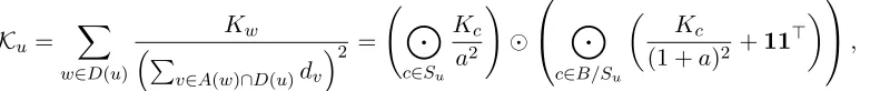
where Ku=Pw∈D(u)
Hw (P
v∈A(w)∩D(u)dv)
2.
The proof is provided in Appendix A.7. It closely follows that for the case of HKL (Bach, 2008).
The summary of the proposed mirror descent based active set algorithm is presented in Algorithm 3. At each iteration, Algorithm (3) verifies optimality of the current iterate by verifying the condition in (15). In case the current iterate does not satisfy this condition, the nodes in sources(Wc) that violate the condition (15) are included in the active set.8 This
takes care of the third requirement of the active set algorithm. The algorithm terminates if the condition (15) is satisfied by the iterate.
In the following, an estimate of the computational complexity of the active set algorithm is presented. Let W be the final active set size. The optimization problem (14) needs to be solved at most W times, assuming the worst case scenario of adding one node per active set iteration. Each run of the mirror descent algorithm requires at most O(log(W)) iterations (Ben-Tal and Nemirovski, 2001; Beck and Teboulle, 2003). A conservative time complexity estimate for computing the gradient ∇g(ηW) by solving a variant of the `ρˆ
-norm MKL problem (13) is O(m3T3W2). This amounts to O(m3T3W3log(W)). As for
the computational cost of the sufficient condition, let z denote the maximum out-degree
of a node in G, i.e., z is an upper-bound on the the maximum number of children of any node in G. Then the size of sources(Wc) is upper-bounded by W z. Hence, a total of
O(ωm2T2W z) operations are required for evaluating the matricesK in (15), whereωis the complexity of computing a single entry in anyK. In all the pragmatic examples of kernels and the corresponding DAGs provided by Bach (2008), ω is polynomial in the training set dimensions. Moreover, caching of K usually renders ω to be a constant (Bach, 2009). Further, the total cost of the quadratic computation in (15) is O(m2T2W2z). Thus the overall computational complexity isO(m3T3W3log(W) +ωm2T2W z+m2T2W2z). More importantly, because the sufficient condition for optimality (Theorem 5) is independent of
ρ, we have the following result:
Corollary 6 In a given input setting, HKL algorithm converges in time polynomial in the size of the active set and the training set dimensions if and only if the proposed mirror descent based active set algorithm (i.e., gHKLMT algorithm) has a polynomial time
conver-gence in terms of the active set and training set sizes.
The proof is provided in Appendix A.10.
In the next section, we present an application of the proposed formulation that illustrate the benefits of the proposed generalizations over HKL.
5. Rule Ensemble Learning
In this section, we propose a solution to the problem of learning an ensemble of decision rules, formally known as Rule Ensemble Learning (REL) (Cohen and Singer, 1999), employing the gHKL and gHKLMT formulations. For the sake of simplicity, we only discuss the single
task REL setting in this section, i.e., REL as an application of gHKL. Similar ideas can be applied to perform REL in multi-task learning setting, by employing gHKLMT. In fact,
we present empirical results of REL in both single and multiple task learning settings in Section 6. We begin with a brief introduction to REL.
If-then decision rules (Rivest, 1987) are one of the most expressive and human readable representations for learned hypotheses. It is a simple logical pattern of the form: IF condi-tion THENdecision. The conditionconsists of a conjunction of a small number of simple boolean statements (propositions) concerning the values of the individual input variables while the decisionspecifies a value of the function being learned. An instance of a decision rule from Quinlan’s play-tennis example (Quinlan, 1986) is:
IFHUMIDITY==normalAND WIND==weakTHENPlayTennis==yes.
The dominant paradigm for induction of rule sets, in the form of decision list (DL) models for classification (Rivest, 1987; Michalski, 1983; Clark and Niblett, 1989), has been a greedy
sequential coveringprocedure.
REL approaches like SLIPPER (Cohen and Singer, 1999), LRI (Weiss and Indurkhya, 2000), RuleFit (Friedman and Popescu, 2008), ENDER/MLRules (Dembczy´nski et al., 2008, 2010) have additionally addressed the problem of learning a compact set of rules that generalize well in order to maintain their readability. Further, a number of rule learners like RuleFit, LRI encourage shorter rules (i.e., fewer conjunctions in the condition part of the rule) or rules with a restricted number of conjunctions, again for purposes of interpretability. We build upon this and define our REL problem as that of learning a small set of simple rules and their weights that leads to a good generalization over new and unseen data. The next section introduces the notations and the setup in context of REL.
5.1 Notations and Setup
Let D = {(x1, y1), . . . ,(xm, ym)} be the training data described using p basic (boolean)
propositions, i.e.,xi∈ {0,1}p. In case the input features are not boolean, such propositions
can be derived using logical operators such as ==,6=,≤or≥over the input features (refer Friedman and Popescu, 2008; Dembczy´nski et al., 2008, for details). Let V be an index-set for all possible conjunctions with the p basic propositions and let φv : Rn 7→ {0,1} denote the vth conjunction in V. Let fv ∈ R denote the weight for the conjunction φv.
Then, the rule ensemble to be learnt is the weighted combination of these conjunctive rules:
F(x) =P
v∈Vfvφv(x)−b, where perhaps many weights (fv) are equal to zero.
One way to learn the weights is by performing a`1-norm regularized risk minimization in
order to select few promising conjunctive rules (Friedman and Popescu, 2008; Dembczy´nski et al., 2008, 2010). However, to the best of our knowledge, rule ensemble learners that iden-tify the need for sparse f, either approximate such a regularized solution using strategies such as shrinkage (Rulefit, ENDER/MLRules) or resort to post-pruning (SLIPPER). This is because the size of the minimization problem is exponential in the number of basic propo-sitions and hence the problem becomes computationally intractable with even moderately sized data sets. Secondly, conjunctive rules involving large number of propositions might be selected. However, such conjunctions adversely effect the interpretability. We present an approach based on the gHKL framework that addresses these issues.
We begin by noting that hV,⊆i is a subset-lattice; hereafter this will be referred to as the conjunction lattice. In a conjunction lattice, ∀ v1, v2 ∈ V, v1 ⊆ v2 if and only if
the set of propositions in conjunction v1 is a subset of those in conjunction v2. As an
example, (HUMIDITY==normal) is considered to be a subset of (HUMIDITY==normal
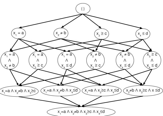
AND WIND==weak). The top node of this lattice is a node with no conjunctions and is also sources(V). Its children, the second level nodes, are all the basic propositions, p in number. The third level nodes, children of these basic propositions, are the conjunctions of length two and so on. The bottom node at (p+ 1)th level is the conjunction of all basic propositions. The number of different conjunctions of length r is pr and the total number of nodes in this conjunction lattice is 2p. Figure (1) shows a complete conjunction lattice withp= 4.
{ }
x1 = a x2 ≠ b x3 ≥ c x4 ≤ d
x1 = a Λ x2 ≠ b
x1=a Λ x2≠b Λ x3≥c x1=a Λ x2≠b Λ x4≤d x1=a Λ x3≥c Λ x4≤d x2≠b Λ x3≥c Λ x ≤d
x1=a Λ x2≠b Λ x3≥c Λ x4≤d x1 = a
Λ
x3 ≥ c
x1 = a Λ x4 ≤ d
x2 ≠ b Λ x3 ≥ c
x2 ≠ b Λ x4 ≤ d
x3 ≥ c Λ x4 ≤ d
Figure 1: Example of a conjunction lattice with 4 basic propositions: (x1 = a), (x2 6=b), (x3 ≥ c) and (x4 ≤ d). The input space consist of four features: x1, x2, x3 and x4. The number of nodes in conjunction lattice is exponential in the number of basic propositions. In this particular example, the number of nodes is 16 (= 24).
5.2 Rule Ensemble Learning with gHKL
The key idea is to employ gHKL formulation (5) with the DAG as the conjunction lattice and the kernels as kv(xi,xj) = φv(xi)φv(xj) for learning an ensemble of rules. Note that
with such a setup, the `1/`ρ block-norm regularizer in gHKL (ΩS(f) =Pv∈VdvkfD(v)kρ)
implies: 1) for mostv∈ V,fv = 0, and 2) for mostv∈ V,fw = 0∀w∈D(v). In the context
of the REL problem, the former statement is equivalent to saying: selection of a compact set of conjunctions is promoted, while the second reads as: selection of conjunctive rules with small number of propositions is encouraged. Thus, gHKL formulation constructs a compact ensemble of simple conjunctive rules. In addition, we setdv =a|Sv|(a >1), where
Sv is the set of basic propositions involved in the conjunction φv. Such a choice further
encourages selection of short conjunctions and leads to the following elegant computational result:
Theorem 7 The complexity of the proposed gHKL algorithm in solving the REL problem, with the DAG, the base kernels and the parametersdv as defined above, is polynomial in the size of the active set and the training set dimensions. In particular, if the final active set size is W, then its complexity is given by O(m3W3log(W) +m2W2p).
The proof is provided in Appendix A.11.
the sparsity pattern allowed by HKL has the following consequence: a conjunction is se-lected only after selecting all the conjunctions which are subsets of it. This, particularly in the context of REL, is psycho-visually redundant, because a rule with k propositional statements, if included in the result, will necessarily entail the inclusion of (2k−1) more gen-eral rules in the result. This violates the important requirement for a small set (Friedman and Popescu, 2008; Dembczy´nski et al., 2008, 2010) of human-readable rules. The gHKL regularizer, with ρ ∈ (1,2), alleviates this restriction by promoting additional sparsity in selecting the conjunctions. We empirically evaluate the proposed gHKL based solution for REL application in the next section.
6. Experimental Results
In this section, we report the results of simulation in REL on several benchmark binary and multiclass classification data sets from the UCI repository (Blake and Lichman, 2013). The goal is to compare various rule ensemble learners on the basis of: (a) generalization, which is measured by the predictive performance on unseen test data, and (b) ability to provide compact set of simple rules to facilitate their readability and interpretability (Friedman and Popescu, 2008; Dembczy´nski et al., 2010; Cohen and Singer, 1999). The latter is judged using i) average number of rules learnt, and ii) average number of propositions per rule. The following REL approaches were compared.
• RuleFit: Rule ensemble learning algorithm proposed by Friedman and Popescu (2008). All the parameters were set to the default values mentioned by the authors. In particular, the model was set in the mixed linear-rule mode, average tree size was set 4 and maximum number of trees were kept as 500. The same configuration was also used by Dembczy´nski et al. (2008, 2010) in their simulations. This REL system cannot han-dle multi-class data sets and hence is limited to the simulations on binary classification data sets. Its code is available atwww-stat.stanford.edu/~jhf/R-RuleFit.html.
• SLI:The SLIPPER algorithm proposed by Cohen and Singer (1999). Following Dem-bczy´nski et al. (2008, 2010), all parameters were set to their defaults. We retained the internal cross-validation for selecting the optimal number of rules.
• ENDER: State-of-the-art rule ensemble learning algorithm (Dembczy´nski et al., 2010). For classification setting, ENDER is same as MLRules (Dembczy´nski et al., 2008). The parameters were set to the default values suggested by the authors. The second order heuristic was used for minimization. Its code is available at www.cs. put.poznan.pl/wkotlowski.
• HKL-`1-MKL:A two-stage rule ensemble learning approach. In the first stage, HKL is employed to prune the exponentially large search space of all possible conjunctive rules and select a set of candidate rules (kernels). The rule ensemble is learnt by employing `1-MKL over the candidate set of rules. In both the stages, a three-fold cross validation procedure was employed to tune the C parameter with values in
{10−3,10−2, . . . ,103}.
• gHKLρ: The proposed gHKL based REL formulation for binary classification
classification,ρ= 2 renders the HKL formulation (Bach, 2008). In each case, a three-fold cross validation procedure was employed to tune the C parameter with values in
{10−3,10−2, . . . ,103}. As mentioned earlier, the parametersdv = 2|v|.
• gHKLMT−ρ: The proposed gHKLMT based REL formulation for multiclass
classi-fication problem. For each class, a one-vs-rest binary classiclassi-fication task is created. Since we did not have any prior knowledge about the correlation among the classes in the data sets, we employed the multi-task regularizer (7) in the gHKLMT primal
formulation (6).
We considered three different values ofρ: 2, 1.5 and 1.1. Its parameters and cross validation details are same as that of gHKLρ. The implementations of both gHKLρ and gHKLMT−ρ are
available athttp://www.cse.iitb.ac.in/~pratik.j/ghkl.
Note that the above methods differ in the way they control the number of rules (M) in the ensemble. In the case of gHKLρ(gHKLMT−ρ),M implicitly depends on the parameters: ρ,
C anddv. SLIhas a parameter for maximum number of rulesMmaxand M is decided via a
internal cross-validation such thatM ≤Mmax. For the sake of fairness in comparison with
gHKLρ, we setMmax= max(M1.5, M1.1), where Mρis the average number of rules obtained
with gHKLρ (gHKLMT−ρ). ENDER has an explicit parameter for the number of rules, which is
also set to max(M1.5, M1.1). In case of RuleFit, the number of rules in the ensemble is
determined internally and is not changed by us.
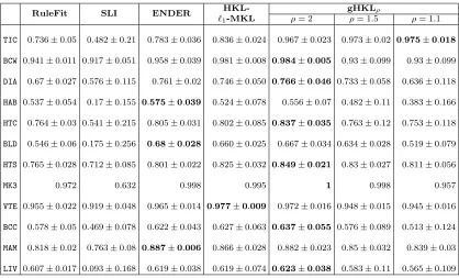
6.1 Binary Classification in REL
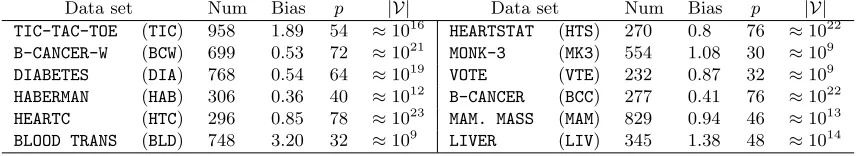
This section summarizes our results on binary REL classification. Table 1 provides the details of the binary classification data sets. For every data set, we created 10 random train-test splits with 10% train data (except for MONK-3 data set, whose train-test split of 122−432 instances respectively was already given in the UCI repository). Since many data sets were highly unbalanced, we report the average F1-score along with the standard deviation (Table 5 in Appendix A.12 reports the average AUC). The results are presented in Table 2. The best result, in terms of the average F1-score, for each data set is highlighted.
Data set Num Bias p |V| Data set Num Bias p |V|
TIC-TAC-TOE (TIC) 958 1.89 54 ≈1016 HEARTSTAT (HTS) 270 0.8 76 ≈1022
B-CANCER-W (BCW) 699 0.53 72 ≈1021 MONK-3 (MK3) 554 1.08 30 ≈109
DIABETES (DIA) 768 0.54 64 ≈1019 VOTE (VTE) 232 0.87 32 ≈109
HABERMAN (HAB) 306 0.36 40 ≈1012 B-CANCER (BCC) 277 0.41 76 ≈1022
HEARTC (HTC) 296 0.85 78 ≈1023 MAM. MASS (MAM) 829 0.94 46 ≈1013
BLOOD TRANS (BLD) 748 3.20 32 ≈109 LIVER (LIV) 345 1.38 48 ≈1014
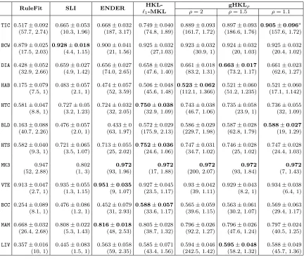
RuleFit SLI ENDER HKL- gHKLρ
`1-MKL ρ= 2 ρ= 1.5 ρ= 1.1
TIC 0.517±0.092 0.665±0.053 0.668±0.032 0.749±0.040 0.889±0.093 0.897±0.093 0.905±0.096∗
(57.7, 2.74) (10.3, 1.96) (187, 3.17) (74.8, 1.89) (161.7, 1.72) (186.6, 1.76) (157.6, 1.72)
BCW 0.879±0.025 0.928±0.018 0.900±0.041 0.925±0.032 0.923±0.032 0.924±0.032 0.925±0.032 (17.5, 2.03) (4.4, 1.15) (21, 1.56) (27,1.03) (30.9, 1) (20, 1.03) (20.4, 1.02)
DIA 0.428±0.052 0.659±0.027 0.656±0.027 0.658±0.028 0.661±0.018 0.663±0.017 0.661±0.023 (32.9, 2.66) (4.9, 1.42) (74.0, 2.65) (47.6, 1.40) (83.2, 1.31) (73.2, 1.17) (62.6, 1.27)
HAB 0.175±0.079 0.483±0.057 0.474±0.057 0.506±0.048 0.523±0.062 0.521±0.060 0.521±0.060 (7.5, 1) (2.1, 1) (52, 3.59) (45.6, 1.48) (112.1, 1.366) (51.2, 1.235) (17.1, 1.142)
HTC 0.581±0.047 0.727±0.05 0.724±0.032 0.750±0.038 0.743±0.038 0.735±0.058 0.736±0.055 (8.8, 1) (3.2, 1.23) (32, 2.05) (32.9, 1.09) (46.7, 1.06) (23.9, 1) (32, 1.09)
BLD 0.163±0.088 0.476±0.057 0.433±0 0.572±0.029 0.586±0.029 0.587±0.028 0.588±0.027
(40.7, 2.26) (2.0, 1) (63, 1.97) (175.9, 2.13) (229.7, 1.98) (62.8, 1.79) (19, 1.29)
HTS 0.582±0.040 0.721±0.065 0.713±0.055 0.752±0.036 0.747±0.031 0.746±0.028 0.747±0.028 (9.3, 1) (3.5, 1.07) (25, 2.02) (24.6, 1.06) (34.7, 1.02) (25, 1.02) (24.4, 1.03)
MK3 0.947 0.802 0.972 0.972 0.972 0.972 0.972
(52, 2.88) (1, 3) (93, 1.96) (17, 1.88) (200, 2.07) (93, 1.84) (7, 1.43)
VTE 0.913±0.047 0.935±0.055 0.951±0.035 0.927±0.045 0.93±0.042 0.929±0.043 0.934±0.038 (2.7, 1) (1.3, 1.15) (9, 1.07) (23.5, 1.17) (39, 1.11) (8.2, 1) (6.4, 1)
BCC 0.254±0.089 0.476±0.086 0.452±0.079 0.588±0.057 0.565±0.059 0.563±0.061 0.569±0.063 (8.1, 1) (1.2, 1) (31, 2.93) (33.6, 1.17) (39.6, 1.15) (30.2, 1.07) (29.4, 1.17)
MAM 0.668±0.032 0.808±0.022 0.816±0.018 0.805±0.028 0.796±0.026 0.796±0.026 0.797±0.024 (26.4, 2.68) (5.3, 1.43) (48, 2.53) (38.7, 1.32) (92.2, 1.27) (47.6, 1.24) (40.5, 1.25)
LIV 0.357±0.016 0.445±0.083 0.563±0.058 0.585±0.071 0.594±0.046 0.595±0.048 0.588±0.049 (10, 1) (1.5, 1) (59, 2.35) (43.4, 1.56) (242.5, 1.42) (58.2, 1.32) (45.7, 1.36)
Table 2: Results on binary REL classification. We report the F1-score along with standard deviation and, in brackets below, the number of the learnt rules as well as the average length of the learnt rules. The proposed REL algorithm, gHKLρ (ρ =
Additionally if the best result achieves a statistically significant improvement over its nearest competitor, it is marked with a ‘*’. Statistical significance test is performed using the paired t-test at 99% confidence. We also report the average number of rules learnt (r) and the average length of the rules (c), specified below each F1-score as: (r, c). As discussed earlier, it is desirable that REL algorithms achieve high F1-score with a compact set of simple rules, i.e., lowr and c.
We can observe from Table 2 thatgHKLρobtains better generalization performance than
state-of-the-art ENDER in most of the data sets with the additional advantage of having rules with smaller number of conjunctions. In fact, when averaged over the data sets,
gHKL1.1 and gHKL1.5 output the shortest rules among all the methods. gHKL1.1 obtains
statistically significant performance in TIC-TAC-TOE data set. Though the generalization obtained by gHKL2 (HKL),gHKL1.5 and gHKL1.1 are similar, the number of rules selected by gHKL2 is always higher thangHKL1.1 (by as much as 25 times in a few cases), hampering its
interpretability.
6.2 Multiclass Classification in REL
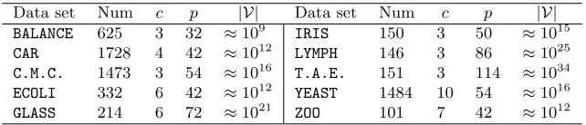
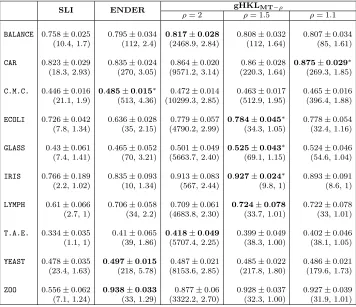
This section summarizes our results on multiclass REL classification. The details of the multiclass data sets are provided in Table 3. Within the data sets, classes with too few instances (< 3) were not considered for simulations since we perform a three-fold cross validation for hyper-parameter selection. The results, averaged over 10 random train-test splits with 10% train data are presented in Table 4. Following Dembczy´nski et al. (2008, 2010), we report the accuracy to compare generalization performance among the algorithms. The number of rules as well as the average length of the rules is also reported to judge the interpretability of the output.
We can observe thatgHKLMT−ρobtains the best generalization performance in seven data
sets, out of which four are statistically significant. Moreover, gHKLMT−1.5 and gHKLMT−1.1
usually select the shortest rules among all the methods. The number of rules as well as the average rule length of gHKLMT−2 is generally very large compared to gHKLMT−1.5 and gHKLMT−1.1. This again demonstrates the suitability of the proposed `1/`ρ regularizer in
obtaining a compact set of simple rules.
Data set Num c p |V| Data set Num c p |V|
BALANCE 625 3 32 ≈109 IRIS 150 3 50 ≈1015
CAR 1728 4 42 ≈1012 LYMPH 146 3 86 ≈1025
C.M.C. 1473 3 54 ≈1016 T.A.E. 151 3 114 ≈1034
ECOLI 332 6 42 ≈1012 YEAST 1484 10 54 ≈1016
GLASS 214 6 72 ≈1021 ZOO 101 7 42 ≈1012
SLI ENDER gHKLMT−ρ
ρ= 2 ρ= 1.5 ρ= 1.1
BALANCE 0.758±0.025 0.795±0.034 0.817±0.028 0.808±0.032 0.807±0.034 (10.4, 1.7) (112, 2.4) (2468.9, 2.84) (112, 1.64) (85, 1.61)
CAR 0.823±0.029 0.835±0.024 0.864±0.020 0.86±0.028 0.875±0.029∗
(18.3, 2.93) (270, 3.05) (9571.2, 3.14) (220.3, 1.64) (269.3, 1.85)
C.M.C. 0.446±0.016 0.485±0.015∗ 0.472±0.014 0.463±0.017 0.465±0.016 (21.1, 1.9) (513, 4.36) (10299.3, 2.85) (512.9, 1.95) (396.4, 1.88)
ECOLI 0.726±0.042 0.636±0.028 0.779±0.057 0.784±0.045∗ 0.778±0.054
(7.8, 1.34) (35, 2.15) (4790.2, 2.99) (34.3, 1.05) (32.4, 1.16)
GLASS 0.43±0.061 0.465±0.052 0.501±0.049 0.525±0.043∗ 0.524±0.046 (7.4, 1.41) (70, 3.21) (5663.7, 2.40) (69.1, 1.15) (54.6, 1.04)
IRIS 0.766±0.189 0.835±0.093 0.913±0.083 0.927±0.024∗ 0.893±0.091 (2.2, 1.02) (10, 1.34) (567, 2.44) (9.8, 1) (8.6, 1)
LYMPH 0.61±0.066 0.706±0.058 0.709±0.061 0.724±0.078 0.722±0.078 (2.7, 1) (34, 2.2) (4683.8, 2.30) (33.7, 1.01) (33, 1.01)
T.A.E. 0.334±0.035 0.41±0.065 0.418±0.049 0.399±0.049 0.402±0.046 (1.1, 1) (39, 1.86) (5707.4, 2.25) (38.3, 1.00) (38.1, 1.05)
YEAST 0.478±0.035 0.497±0.015 0.487±0.021 0.485±0.022 0.486±0.021 (23.4, 1.63) (218, 5.78) (8153.6, 2.85) (217.8, 1.80) (179.6, 1.73)
ZOO 0.556±0.062 0.938±0.033 0.877±0.06 0.928±0.037 0.927±0.039 (7.1, 1.24) (33, 1.29) (3322.2, 2.70) (32.3, 1.00) (31.9, 1.01)
Table 4: Results on multiclass REL classification. We report the accuracy along with stan-dard deviation and, in the brackets below, the number of learnt rules as well as the average length of the learnt rules. The proposed REL algorithm,gHKLMT−ρ, obtains
the best generalization performance in most data sets. In addition, forρ= 1.5 and 1.1, our algorithm learns a smaller set of more compact rules than state-of-the-art
ENDER. The ‘*’ symbol denotes statistically significant improvement. The results are averaged over ten random train-test splits.
7. Summary
This paper generalizes the HKL framework in two ways. First, a generic `1/`ρblock-norm
regularizer,ρ∈(1,2), is employed that provides a more flexible kernel selection pattern than HKL by mitigating the weight bias towards the kernels that are nearer to the sources of the DAG. Secondly, the framework is further generalized to the setup of learning a shared feature representation among multiple related tasks. We pose the problem of learning shared fea-tures across the tasks as that of learning a shared kernel. An efficient mirror descent based active set algorithm is proposed to solve the generalized formulations (gHKL/gHKLMT).
An interesting computational result is that gHKL/gHKLMT can be solved in time
where HKL has not been previously explored. We pose the problem of learning an en-semble of propositional rules as a kernel learning problem. Empirical results on binary as well as multiclass classification for REL demonstrate the effectiveness of the proposed generalizations.
Acknowledgments
We thank the anonymous reviewers for the valuable comments. We acknowledge Chiran-jib Bhattacharyya for initiating discussions on optimal learning of rule ensembles. Pratik Jawanpuria acknowledges support from IBM Ph.D. fellowship.
Appendix A.
In the appendix section, we provide the proofs of theorems/lemmas referred to in the main paper.
A.1 Lemma 26 of Micchelli and Pontil (2005)
Let ai ≥0, i = 1, . . . , d, 1≤r <∞ and ∆d,r =
n
z∈Rd |z≥0,Pd
i=1zri ≤1
o
. Then, the following result holds:
min
z∈∆d,r
d
X
i=1 ai
zi
=
d
X
i=1 a
r r+1
i
!1+1r
.
The minimum is attained at
zi =
a
1
r+1
i
Pd
j=1a
r r+1
j
1r
∀i= 1, . . . , d.
The proof follows from Holder’s inequality.
A.2 Proof of Lemma 1
Proof Applying the above lemma (Appendix A.1) on the outermost`1-norm of the
regu-larizer ΩT(f1, . . . , fT)2 in (6), we get
ΩT(f1, . . . , fT)2 = min γ∈∆1
X
v∈V
d2v γv
X
w∈D(v)
(Qw(f1, . . . , fT))ρ
2
ρ
,
where ∆1 =
z∈R|V| |z≥0,P
v∈Vzv ≤1 . Reapplying the above lemma on the
individ-ual terms of the above summation gives
X
w∈D(v)
(Qw(f1, . . . , fT)2)
ρ
2
2
ρ
= min
λv∈∆vρˆ X
w∈D(v)
Qw(f1, . . . , fT)2
λvw
where ˆρ = 2−ρρ and ∆vr = n
z∈R|D(v)| |z≥0,P
w∈D(v)zrw≤1
o
. Using the above two re-sults and regrouping the terms will complete the proof.
A.3 Re-parameterization of the Multi-task Regularizer in (8)
The gHKLMT dual formulation (10) follows from the representer theorem (Sch¨olkopf and
Smola, 2002) after employing the following re-parameterization in (8). Define f0w = T+1µPT
t=1ftw and ftw=ftw−f0w. Then,Qw(f1, . . . , fT) in (8) may be
rewritten as:
Qw(f1, . . . , fT) = µkf0wk2+ T
X
t=1
kftwk2
!12
.
Further, construct the following feature map (Evgeniou and Pontil, 2004)
Φw(x, t) = (
φw(x)
√
µ , 0|, . . . ,{z 0}
for tasks before t
, φw(x), 0, . . . ,0
| {z }
for tasks after t
) (16)
and definefw = (
√
µf0w, f1w, . . . , fT w).
With the above definitions, we rewrite the gHKLMT primal regularizer as well as the
prediction function: Qw(f1, . . . , fT)2 =kfwk2 and Ft(x) =Pw∈Vhfw,Φw(x, t)i −bt ∀t. It
follows from Lemma 1 that the gHKLMT primal problem based on (8) is equivalent to the
following optimization problem:
min
γ∈∆1
min
λv∈∆vρˆ ∀v∈V min
f,b
1 2
X
w∈V
δw(γ, λ)−1kfwk2+C T
X
t=1
m
X
i=1
`(yti, Ft(xti)), (17)
wheref = (fw)w∈V and b= [b1, . . . , bT].
A.4 Motivation for the Active Set Algorithm
Lemma 8 The problem (12) remains the same whether solved with the original set of vari-ables (η) or when solved with only thoseηv 6= 0 at optimality.
Proof The above follows from the following reasoning: a) variables η owe their presence in (12) only via ζ(η) functions, b) (ηv = 0) ⇒ (ζw(η) = 0 ∀w ∈ D(v)), c) Let (η0, α0) be
an optimal solution of the problem (12). If ζv(η0) = 0 andηv0 6= 0, then (η∗, α0) is also an
optimal solution of the problem (12) whereη∗w =ηw0 ∀w∈ V \vandηv∗= 0, and d) min-max interchange in (12) yields an equivalent formulation.
Lemma 9 The following min-max interchange is equivalent:
min
η∈∆1
max
αt∈S(yt,C)∀t ¯
G(η, α) = max
αt∈S(yt,C)∀t min
η∈∆1
¯
where
¯
G(η, α) =1>α−1
2 X
w∈V
ζw(η)
α>YHwYα
ρ¯ !1ρ¯
.
Proof Note that G(η, α) is a convex function in η and a concave function in α. The min-max interchange follows from Sion-Kakutani minimax theorem (Sion, 1958).
A.5 Proof of Theorem 3
Before stating the proof of Theorem 3, we first prove the results in Lemma 10, Proposi-tion 11 and Lemma 12, which will be employed therein (also see Bach, 2009, Lemma 10 and Proposition 11).
Lemma 10 Let ai >0 ∀i= 1, . . . , d,1< r <∞ and ∆1 =
n
z∈Rd | z≥0,Pd
i=1zi ≤1
o
. Then, the following holds true:
min
z∈∆1
d
X
i=1
aizri = d
X
i=1 a
1 1−r
i
!1−r
and the minimum is attained at
zi=a
1 1−r
i
d
X
j=1 a
1 1−r
i
−1
∀ i= 1, . . . , d.
Proof Take vectorsu1andu2as those with entriesa
1
r
i zianda
−1
r
i ∀i= 1, . . . , drespectively.
The result follows from the Holder’s inequality: u>1u2 ≤ ku1krku2k r
r−1. Note that if any
ai= 0, then the optimal value of the above optimization problem is zero.
Proposition 11 The following convex optimization problems are dual to each other and there is no duality gap:
max
γ∈∆1
X
w∈V
δw(γ, λ)Mw, (18)
min
κ∈L maxu∈V X
w∈D(u)
κ2uwλuwMw
d2
u
, (19)
where L = {κ ∈ R|V|×|V| | κ ≥ 0, P
v∈A(w)κvw = 1, κvw = 0 ∀v ∈ A(w)c, ∀w ∈ V},
∆1=
z∈R|V| |z≥0,P
v∈Vzv ≤1 andMw ≥0 ∀w∈ V.
Proof The optimization problem (19) may be equivalently rewritten as:
min
κ∈L minA A, subject to A≥
X
w∈D(u)
κ2uwλuwMw
d2
u